Feature-based Visual Odometry and Featureless

Feature-based Visual Odometry and Featureless Place Recognition for SLAM in 2.5D Environments Michael Milford, David McKinnon, Michael Warren, Gordon Wyeth, Ben Upcroft School of Engineering Systems Queensland University of Technology [email protected]

Abstract In this paper we present work integrating the robust sequence-based recognition capabilities of the RatSLAM system with the accurate 3D metric properties of a multicamera visual odometry system. The RatSLAM system provides scene sequence recognition capabilities that are not feature dependent, while the multicamera visual odometry system provides accurate and metric 3D motion information which only relies on being able to detect features consistently over short periods of time. We present mapping results using both the new integrated system and the previous RatSLAM-only system for a 1300 metre 3D dataset acquired in a busy and challenging environment. The integration of an accurate visual odometry system results in significant improvements in map quality.

1 Introduction Feature-based visual SLAM and navigation systems are rapidly advancing in capabilities relative to traditional range sensor-based SLAM systems. State of the art systems such as FabMAP [1] and FrameSLAM [2] are able to map large environments [3] using only visual sensing. A complete visual SLAM system incorporates two main components – some form of place learning and recognition system which provides localization, and some form of self-motion processing which calculates the motion of the visual sensor or robot. Each component places different requirements on the visual processing system which limit the applicability of the overall system in different ways. The majority of visual SLAM and visual odometry techniques today rely on some form of feature detection, whether that be SIFT [4], SURF [5], PIRF [6] or some other feature detector. To obtain accurate visual odometry, features in an image must be detected reliably and accurately over a short period of time to generate feature tracks. In the case of multicamera approaches, feature correspondences must also be correct and robust. For localization however, common features must be detectable under all possible conditions. This is an additional constraint that limits the general applicability of most visual SLAM systems available today. Environmental

changes caused by lighting, weather and geometry are challenges that are not handled well by current systems. Yet these are challenges that must be addressed to achieve one of the “hot” goals in robotics today - the challenge of lifelong or persistent autonomy for robots. An alternative visual SLAM system is the RatSLAM brain-based system [7], which uses computational models of the part of the rodent brain thought to process navigation to enable navigation on robots. RatSLAM performs localization by recognizing sequences of familiar visual input. This sequence-based recognition, in combination with the neuronal dynamics emulated in the RatSLAM neural networks, has enabled RatSLAM to successfully perform SLAM over a wide range of environments and robotic platforms using very low resolution, poor quality visual input. RatSLAM typically takes as input 1000 pixel images or simple image intensity profiles, yet is able to successfully map large outdoor environments [8] and changing indoor environments over long periods of time [9]. However, current implementations of RatSLAM are unable to produce globally metric maps, and have very limited means of generating metric 3D information [10]. In this paper, we describe research and experimental testing of our attempts to combine the accurate, 3D metricity of feature-based visual odometry techniques with the featureless localization capabilities of RatSLAM. The paper proceeds as follows. In Section 2 we provide background on visual odometry and place recognition techniques. Section 3 describes the specific multicamera visual odometry algorithms and RatSLAM implementation utilized in this work. The experimental setup is provided in Section 4, while Section 5 presents mapping results. In Section 6 we discuss the implications of this research and provide some directions for future work.

2 Background 2.1 Visual Odometry Visual odometry (VO) is critical for any robotic system forming accurate spatial maps of its surrounding environment and successfully localising within those maps; the classical SLAM problem. Recent developments in image processing and computer vision have resulted in

autonomous platforms using vision as a primary sensor. Cameras are inexpensive relative to laser range finders and have a far higher rate of information output. Although GPS units are capable of providing accurate location estimates, they are subject to difficulties indoors, in urban environments and heavily forested areas. Additionally, the resolution of the spatial location estimates from low-cost GPS sensors (in the range of 1 to 10 metres) is not adequate for visual scene estimation, where precise knowledge of camera position is essential. There have been a number of different groups that have presented successful approaches for VO. Some initial efforts were focused on the use of single uncalibrated moving cameras [11]. Issues such as projective drift in addition to the very difficult task of practical auto-calibration, led subsequent authors towards a focus on calibrated methods for visual motion estimation [12, 13]. In [14] both single camera and stereo-rig approaches to the task of VO are presented. The conclusions of [14] indicate that the single camera method is less reliable due to inherent ambiguities in calculating the essential matrix between pairs of images to initialise the structure and motion [15]. These ambiguities have been further verified for some specific motions such as pure sideways translation [16]. Later work focuses on stereo camera rigs for the calculation of VO [2, 17, 18]. These approaches have been successful in demonstrating that accurate VO can be obtained on a robotic platform at high frame-rates both with [18] and without the use of additional GPS and INS information. In [17, 19] it is reported that a purely vision based method is capable of estimating the total motion of a robotic platform within 1-2 meters over ~1km trajectories without the use of loop closure detection. 2.2 Visual Place Recognition and SLAM There are a number of state of the art visual SLAM systems in existence today with performance approaching or exceeding laser range-based techniques [2-7]. The focus of much of the work has been to create accurate metric maps of an environment, and the majority of research reported is done on datasets offline (but often at real-time speed), rather than during live robot experiments. A standard robot vision dataset consists of high quality, high resolution forward facing or panoramic imagery. Impressive mapping results have been achieved using vision as the primary mapping sensor, including mapping of a 1000 km long journey [2]. Most of these visual navigation systems rely on some form of feature detector such as Scale-Invariant Feature Transforms (SIFT) [11] and Speeded Up Robust Features (SURF) [12]. These feature detectors are state of the art and exhibit some degree of invariance to scaling, rotation and illumination. However, when environmental change becomes significant [13] they inevitably fail; there is currently no “super” feature which is robustly detectable across all environment conditions and times. However, features are generally reliably detectable over short time frames, which is the motivation for using a feature-based

visual odometry system in this work but a featureless place recognition system.

3 Approach In this section we provide details for the SLAM and Visual Odometry systems used for the work presented in this paper. 3.1 RatSLAM System RatSLAM is a robotic visual SLAM system inspired by models of the neural processes underlying navigation in the rodent brain. It has been deployed on a range of robot and vehicle platforms in many different environments [8, 9, 20], but always on ground-based robots. RatSLAM consists of three major components – a continuous attractor neural network known as the pose cells, a graphical map known as the experience map, and a set of local view cells (Fig. 1). The pose cell network encodes the robot’s pose state, and performs the role of filtering self-motion and visual information. The local view cells encode distinct visual scenes or templates – each cell becomes associated with a distinct visual template. The experience map provides a topologically correct and locally metric map of the environment for use in navigation. In this paper, we use the experience map to show the utility of the visual recognition system in performing SLAM. More detailed descriptions of the RatSLAM system can be found in [8, 9]. 3.2 Extending RatSLAM to 2.5D To extend the mapping output of the RatSLAM system to work in 3D, we added an additional altitude parameter to nodes in the experience map, and an additional change in altitude measure to links between nodes. The map correction algorithm was also updated to distribute altitude errors upon loop closure throughout the map, in much the same way that errors in (x, y) position are distributed throughout the map.

Fig. 1. The RatSLAM system consists of the pose cells, which perform filtering of visual input from the local view cells which encode visual scenes in the environment. The output from both the pose and local view cells drives the creation of an experience map, a topological, locally metric graphical map of the environment.

The filtering component of RatSLAM, the pose cells, was retained as a 3D structure encoding (x, y, θ). Expanding this structure to handle unconstrained 6DOF motion would result in a computationally intractable network. However, for a wide range of robotic and computer vision applications, motion occurs

predominantly in a 2.5D manner. For example, a person walking around a university campus will predominantly be attached to a ground plane, whether that be the ground or the 10th floor of a building. Many environments are path-based and hence most motion is constrained to a small subset of the entire 3D space. The implications of retaining the existing pose cell structure is firstly that the algorithm must rely on visual sequences to disambiguate paths that overlap in (x, y) space but are separated by altitude, which the RatSLAM system is designed to do. Secondly, because we do not extract relative poses in 3D in a localization sense, we rely on the metricity of the visual odometry technique to make the overall map metric. 3.3 Visual Odometry Feature Detection and Matching Over the next two sections we briefly describe the main methods employed within our visual odometry technique for acquiring metric information. One of the most important aspects of visual odometry is feature detection and matching. There are several considerations involved with selecting a method for feature detection. Firstly, the method utilised should be both fast and capable of providing repeatable sets of features for tracking between frames. Secondly, the method should provide features that can potentially be rematched if the robotic platform revisits an area to achieve loop closures. For this system a range of different methods were tried. The method best suiting the given criteria for our algorithm is a GPU implementation of the SURF detector [21] due to its scale and rotation invariance and relatively low computational cost. In order to achieve reliable estimates of the camera pose it is very important to have a set of salient features that are well distributed in the image. By simply lowering the thresholds on the feature detector it is natural to obtain a proliferation of features in highly salient regions of the image [17]. To ensure that any given region of an image does not contribute an excessive number of features, a bucketing scheme was applied to threshold a region's total count. This results in an even distribution of features where only the most locally salient are retained. This promotes the likelihood that subsequent estimates of the camera's pose will not be based from sets of points that are all in the same region of the scene. The tracking process proceeds by detecting SURF features in all of the images at each time-point. A GPU-based feature matching scheme is then used to match features from the base camera ( , ) to those at the previous time-point ( , ). Successful matches are those where the ratio of the Euclidean distances between the best and second best descriptor candidates exceeds 0.6 [22]. To locate the corresponding features in the other cameras, a GPU-based guided matching scheme is used. The selected corresponding feature is the one with the best matching descriptor within a set pixel distance of the epipolar line transferred from the base image. This constraint minimises the search space significantly by forcing matches to occur only in a small region of the image rather than the whole set of pixels. Not only does this approach improve speed but also improves accuracy

by preventing spurious matches. If the position of the scene feature is known from previously initialised time-points, its depth along the corresponding epipolar line is known precisely, reducing the search space to an even smaller section of the image. Ideally, we require only a small set of features (20-50) to be tracked between images. However, when a multiple-camera rig is used we may also require that each tracked corner be located in at least two of the cameras at each time-point. This condition results in a large majority of the extracted features not being suitable for the generation of pose estimates because they cannot be reliably tracked between cameras and/or at different time-points. 3.4 Pose Estimation Given that a set of features has been tracked successfully from the previous set of frames, it is now possible to estimate the new location of the camera rig. The most common method [14, 17, 18] is to determine the camera's pose from the existing scene structure using calibrated 3-point pose estimation [23]. This has the advantage of using the well conditioned scene structure from previous time-points, without having to rely as heavily on the new track data being introduced. The particular algorithm used in this case is from [24] and is combined with a MLESAC [25] hypothesis and test paradigm in order to account for incorrect feature tracks and erroneous scene structure. The computation of the camera's pose is achieved by randomly selecting four of the previously tracked scene point - image feature pairs using Monte-Carlo sampling. Note that this further enforces that the set of points used to generate a pose estimate are disparately located within the scene. Three of these pairs are then used to generate between one and three real solutions for the pose of the base camera. The fourth pair disambiguates these solutions by selecting the one with lowest reprojection error in the base image. Within the MLESAC routine, further accelerations are achieved by using a novel modification of the , test [26] to allow for early detection of poor pose estimates. This greatly reduces the need to calculate all the reprojection errors for unlikely pose hypotheses. The modification replaces the chi-squared test from [26] with a test that the average (Huber) truncated cost of the reprojection error for the d tested points does not exceed the average reprojection error of the best solution found so far. This modification attempts to enforce that only improved estimates for the camera's pose be tested in full. 3.5 Visual Templates Figure 2 shows the RatSLAM visual template learning system, and the patch locations used for the patch-based visual odometry. Template differences, D, between the current candidate template i and each learnt template j are calculated using a normalized sum of pixel intensity differences performed over a moving sub frame in the resolution reduced images:

Dj 

min

x , y[  , ]

g x, y , i, j 

(1)

where σ is the template offset range, and g( ) is given by: g x, y , i, j  

1 s2

  p s

s

x 0 y 0

i x  x , y  y

 p xj, y



(2)

where s is the size of the template sub frame. These template differences are normalized by the current recognition threshold, Tj, of each template to calculate the template with the smallest normalized difference. The current template index, k, is calculated by:

arg min D j T j k   j[ 0,n ]  i

D j Tj  1 min D T   1

closures and a range of movement over elevated pathways, sloped ramps and stairwells. The dataset was gathered during a busy weekday, with a large number of students moving around in the cameras’ field of view in many parts of the dataset, as can be seen by the camera snapshots in Figure 4. The multicamera situation was even more challenging in that the cameras had a smaller field of view than the snapshot camera used to perform localization.

(3)

where n is the number of learnt templates, and i is the index of the current template candidate. If no templates are close enough to the current scene, the current candidate template i is added to the learnt templates.

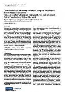
Fig. 3. The testing environment and approximate camera trajectory projected onto the ground plane. The shaded areas indicated by A and B show the subset schematics in Figures 9 and 10 respectively, which have more precisely drawn camera trajectories. Source NearMaps.

Fig. 2. The visual template learning and patch-based visual odometry systems. Each scene is resolution reduced, grayscaled and smoothed then compared to a library of learnt templates.

The patch-based visual odometry is covered in more detail in [10] – the two patches shown in the top part of Figure 2 show the patch locations, which are tracked for movement. The detected movement is turned into camera yaw motion using the top patch, and into camera translation in the (x, y) ground plane using the bottom patch. For this work it is assumed the camera maintains a reasonably neutral pitch. The scale factor for translational speed ν is achieved by calibrating on a short dataset, while the yaw gain constant ς is calculated from the field of view.

4 Experimental Setup In this section, we describe the testing environment, camera platform and image pre-processing. 4.1 Testing Environment

The testing environment was part of the Queensland University of Technology Gardens Point campus, shown in Figure 3. The approximate path taken by the camera is shown on the map. The route taken involved several loop

Fig. 4. Snapshots of the environment, showing the highly dynamic nature of the testing environment (faces blurred to preserve privacy).

4.2 Camera Platform

The multicamera rig consisted of four Firewire 1394B colour Point Grey Flea 2 cameras and a Panasonic TZ-7 consumer snapshot camera. Images were captured synchronously by the Flea 2 cameras using timing inputs from the Firewire bus in compliance with the Firewire protocol. The cameras have relatively long focal length lenses (6.0mm) for the application with a FOV of approximately 43° × 33°. The small FOV complicates the recovery of VO but this can be mitigated by the combined effect of the four cameras. The cameras acquire

time-synchronised, greyscale images at a resolution of 640 × 480 pixels at 30Hz over the firewire bus. The logging software monitors the images entering the computer to ensure synchronisation across all four cameras. Any images that are not synchronised are dropped. Images from the TZ-7 were obtained at 50fps and 1280 × 720 pixels.

5.1 Place Recognition

The RatSLAM template matcher performs well on the dataset, and is able to recognize coherent sequences of visual templates each time the camera repeated a part of the route, despite the highly populated nature of parts of the environment. Figure 6 shows the templates as they are learned and recalled over time. Just over 1800 templates were learned. Repeated sections of route are shaded. Recall was high during repeated sections, with occasional failures in recall such as around frame 7000 in the figure.

Fig. 5. The data acquisition testing rig consisting of four Point Grey Flea 2 cameras for the multicamera visual odometry and an additional Panasonic TZ-7 consumer snapshot camera.

4.3 Image Pre-Processing

Images from the TZ-7 camera were converted to grayscale, and resolution reduced to an intermediate resolution of 320 × 240 pixels (used for the patch-based visual odometry shown in Figure 2). The images were then resolution reduced again and Gaussian blurred (radius 5) to form 32 × 32 images, which formed the basis of the visual templates used by the RatSLAM system described in Section 3.6. Frames from the 4 Point Grey cameras were decimated by a factor of 5 before being used to perform multicamera visual odometry. 4.4 System Parameters

Table I provides a list and description of all the key visual algorithm parameters and values. RatSLAM parameter values were as given in [10].

Fig. 6. Template learning and recall.

5.2 Visual Odometry 2D

Figure 7 shows the calculated camera trajectory projected onto an approximate 2D ground plane using the (a) original patch odometry method and the (b) multicamera visual odometry. The multicamera visual odometry method clearly reduced drift, with a final error in position of approximately 25 metres, compared with a final error of about 83 metres using the patch odometry method. It is clear that some form of loop closure is required in both cases to improve map accuracy.

TABLE I PARAMETER LIST Parameter

Value

Description

r ς ν ρ s σ

32 pixels 0.225 °/pixel 0.2072 m/pixel 10 pixels 24 pixels 4 pixels

Odometry patch size Yaw gain constant Translational speed constant Patch-odo offset range Template sub frame size Template offset range

5 Results In this section we present visual odometry, template recall and mapping results in both 2D and 3D. Obtaining accurate 3D ground truth is very difficult in large dynamic and cluttered outdoor environments and is a goal we are currently working towards using survey data for our campus. However, for this paper we present maps side by side for qualitative comparison in both 2D and 3D.

Fig. 7. (a) RatSLAM patch-based and (b) multicamera-based visual odometry without loop closure.

5.3 Experience Maps in 2D and 3D

Figure 8 show the experience map output by the RatSLAM system when using (b) multicamera visual odometry and (c) patch odometry, respectively. Viewed globally and in 2D, it is not immediately obvious whether the multicamera visual odometry is improving matters significantly, with the exception of providing accurate scaling – the patch odometry based map is approximately 33% too small.

Consequently, we examine two parts of the map in closer detail both in 2D and 3D to shed further light on the comparison.

Fig. 8. (a) Original camera trajectory. (b) Experience map using multicamera visual odometry. (c) Experience map using patch-based visual odometry. Two main map dimensions are shown, including the ground truth distances in (a).

5.4 2D and 3D Experience Map Submaps

Figure 9 and 10 show 2D (first column of each figure) and 3D (second column) enlarged subsections of the experience maps. Figure 9 shows a loop in the environment which consisted of climbing a short set of stairs and then walking down a gradual downhill ramp. The 2D experience map using RatSLAM and multicamera visual odometry closely matches the actual 2D camera trajectory more closely than the patch-based technique. In 3D the difference is even clearer, with the steep climb up the stairs evident in the top part of Figure 9f. What should be straight lines are jagged and irregular in Figure 9e, showing that patch odometry is particularly unsuitable in 3D. There is also a clear divergence of paths in Figure 9e which is not present in 9f – RatSLAM is able to better bind together repeated camera paths (which should overlap in 3D space) when provided with the multicamera visual odometry. This trend was qualitatively observed in many parts of the dataset. Figure 10 shows a part of the route which consisted of walking along an elevated walkway, down a set of stairs, and then back along a path underneath and offset to the side of the walkway. Here the difference in the 2D maps is not as great – while the multicamera visual odometry gets the relative offset between the “top path” and “bottom path 1” correct, there is an error in the stair projection. In 3D once again, the difference is very marked. In this case, the patch odometry method actually incorrectly inverts the vertical positions of the “top path” and “bottom path 1”.

Fig. 9. (a) Approximate ground truth and (b) 2D patch-based visual odometry experience submap and (c) multicamera-based visual odometry experience submap. (d-f) The same location but in 3D.

develop methods for enabling the loop closure provided by RatSLAM to modify the visual odometry system parameters, rather than just correcting the resulting map as in the current system. On the robotic front, we are looking to test the utility of these maps by deploying quadrotors as delivery bots, which will use the maps to navigate. Ultimately the test will be whether the integrated system is able to reliably generate maps under a wide range of environmental conditions, and whether users such as humans and robots will be able to use these maps to perform useful tasks in an effective manner.

References

Fig. 10. (a) Approximate ground truth and (b) 2D patch-based visual odometry experience submap and (c) multicamera-based visual odometry experience submap for a second location. (d-f) The same location but in 3D.

6 Discussion and Future Work The experimental results presented in this paper demonstrate that the addition of an accurate and metric visual odometry system to RatSLAM, which has never been done before, improves the quality of the experience map, especially when viewed in 3D. It is interesting to note that the apparent difference between patch-based and multicamera visual odometry, when viewed projected onto the 2D ground plane, is not clear (aside from scaling) but becomes obvious when viewed in 3D. We will continue to develop the integrated system, and will gather larger, more challenging datasets and compare its map generation performance to other state of the art systems from both a metricity and also robustness under varying environmental conditions standpoint. Secondly, we will continue to develop methods for acquiring dataset geometric ground truth measures that are applicable in large environments. We particularly are interested in performing mixed indoor and outdoor experiments, which clearly preclude the use of a system such as VICON. Thirdly, regardless of ground truth accuracy, we are interested in to what degree a map needs to be metrically accurate in 3D in order to be useful. Towards that end, we are looking at experiments with both humans and robots making use of the generated maps to perform useful tasks such as deliveries and tour guiding. In particular, we would look to expand on our work in 2D delivery robotics, where we have already shown that the map need not be metric in order to carry out the task effectively [9]. A fourth area of investigation will be to

[1] M. Cummins and P. Newman, "FAB-MAP: Probabilistic Localization and Mapping in the Space of Appearance," International Journal of Robotics Research, vol. 27, pp. 647-665, 2008. [2] K. Konolige and M. Agrawal, "FrameSLAM: From Bundle Adjustment to Real-Time Visual Mapping," IEEE Transactions on Robotics, vol. 24, pp. 1066-1077, 2008. [3] M. Cummins and P. Newman, "Highly scalable appearance-only SLAM - FAB-MAP 2.0," presented at Robotics: Science and Systems, Seattle, United States, 2009. [4] D. G. Lowe, "Distinctive Image Features from Scale-Invariant Keypoints," International Journal of Computer Vision, vol. 60, pp. 91-110, 2004. [5] H. Bay, T. Tuytelaars, and L. Van Gool, "SURF: Speeded Up Robust Features," in Computer Vision – ECCV 2006, 2006, pp. 404-417. [6] A. Kawewong, N. Tongprasit, S. Tangruamsub, and O. Hasegawa, "Online and Incremental Appearance-based SLAM in Highly Dynamic Environments," The International Journal of Robotics Research, 2010. [7] M. J. Milford, G. Wyeth, and D. Prasser, "RatSLAM: A Hippocampal Model for Simultaneous Localization and Mapping," presented at IEEE International Conference on Robotics and Automation, New Orleans, USA, 2004. [8] M. Milford and G. Wyeth, "Mapping a Suburb with a Single Camera using a Biologically Inspired SLAM System," IEEE Transactions on Robotics, vol. 24, pp. 1038-1053, 2008. [9] M. Milford and G. Wyeth, "Persistent Navigation and Mapping using a Biologically Inspired SLAM System," International Journal of Robotics Research, vol. 29, pp. 1131-1153, 2010. [10] M. Milford, F. Schill, P. Corke, R. Mahony, and G. Wyeth, "Aerial SLAM with a Single Camera Using Visual Expectation," presented at International Conference on Robotics and Automation, Shanghai, China, 2011. [11] M. Pollefeys, L. Van Gool, M. Vergauwen, F. Verbiest, K. Cornelis, J. Tops, and R. Koch, "Visual modeling with a hand-held camera," International

Journal of Computer Vision, vol. 59, pp. 207-232, 2004. [12] C. F. Olson, L. H. Matthies, H. Schoppers, and M. W. Maimone, "Robust Stereo Ego-motion for Long Distance Navigation," presented at Conference on Computer Vision and Pattern Recognition, Hilton Head, United States, 2000. [13] P. Corke, D. Strelow, and S. Singh, "Omnidirectional visual odometry for a planetary rover," presented at International Conference on Intelligent Robots and Systems, Sendai, Japan, 2004. [14] D. Nister, O. Naroditsky, and J. Bergen, "Visual Odometry," presented at Computer Vision and Pattern Recognition, Washington DC, United States, 2004. [15] D. Nister, "An efficient solution to the five-point relative pose problem," IEEE Transactions on Pattern Analysis and Machine Intelligence, vol. 26, pp. 756-777, 2004. [16] D. Nister and C. Engels, "Estimating global uncertainty in epipoloar geometry for vehicle-mounted cameras," presented at SPIE, San Diego, United States, 2006. [17] C. Mei, G. Sibley, M. Cummins, P. Newman, and I. Reid, "A constant time efficient stereo slam system," presented at British Machine Vision Conference, London, 2009. [18] K. Konolige and M. Agrawal, "Large scale visual odometry for rough terrain," presented at International Symposium on Robotics Research, Hiroshima, Japan, 2007. [19] M. Warren, D. McKinnon, H. He, and B. Upcroft, "Unaided stereo vision based pose estimation,"

presented at Australasian Conference on Robotics and Automation, Brisbane, Australia, 2010. [20] D. Prasser, M. Milford, and G. Wyeth, "Outdoor simultaneous localisation and mapping using RatSLAM," presented at International Conference on Field and Service Robotics, Port Douglas, Australia, 2005. [21] P. Furgale and C. H. Tong, "GPUSurf - speeded up SURF," 2010. [22] D. G. Lowe, "Object recognition from local scale-invariant features," presented at International Conference on Computer Vision, Kerkyra, Greence, 1999. [23] B. M. Haralick, C. N. Lee, K. Ottenberg, and M. Nolle, "Review and analysis of solutions of the three point perspective pose estimation problem," International Journal of Computer Vision, vol. 13, pp. 331-356, 1994. [24] M. A. Fischler and R. C. Bolles, "Random sample consensus: a paradigm for model fitting with applications to image analysis and automated cartography," Communications of the ACM, vol. 24, 1981. [25] P. H. S. Torr and A. Zisserman, "MLESAC: a new robust estimator with application to estimating image geometry," Computer Vision Image Understanding, vol. 78, pp. 138-156, 2000. [26] J. Matas and O. Chum, "Randomized ransac with Td,d test," British Machine Vision Computing, vol. 22, pp. 837-842, 2002.