Feature Selection and Ranking Filters. - CiteSeerX

Feature Selection and Ranking Filters. Włodzisław Duch1,2 , Tomasz Winiarski1 , Jacek Biesiada3 , and Adam Kachel 3 1

3

Dept. of Informatics, Nicholaus Copernicus University, Toru´n, Poland http://www.phys.uni.torun.pl/kmk 2 School of Computer Engineering, Nanyang Technological University, Singapore Division of Computer Methods, Dept. of Electrotechnology, The Silesian University of Technology, Katowice, Poland

Abstract. Many feature selection and feature ranking methods have been proposed. Using real and artificial data an attempt has been made to compare some of these methods. The "feature relevance index" used seems to have little effect on the relative ranking. For continuous features discretization and kernel smoothing are compared. Selection of subsets of features using hashing techniques is compared with the "golden standard" of generating and testing all possible subsets of features.

1 Introduction Attention is the basic mechanism that the brain is using to select relevant information for further processing. Without initial selection of information the brain would be overflooded with infromation and could not function. In many applications of computational intelligence methods the situation is similar: large number of features irrelevant to a given taks is provided, making the analysis of data very difficult. Many algorithms for filtering information have been devised in the past, either ranking the relative importance of features, or selecting subsets of features [1, 2]. Information theory is most often use as a basis for such methods, but feature relevance indices based on correlation, purity of classes or consistency are also used. Unfortunately relative advantages and weaknesses of these methods are not know. Feature ranking methods evaluate the relevance of each feature independently, thus leaving potentially redundant features. Feature selection methods search for best subsets of features, offering larger dimensionality reduction. Exhaustive search with performance evaluation on all possible subsets of features provides the golden standard. Although for larger number of features n it is not realistic (the number of all subsets is 2n ), sometimes it may be performed using only the subset of high-ranking features. Finding useful subsets of features is equivalent to assigning binary weights to inputs, so feature and subset selection is a special case of feature transformation. Some classification and approximation methods may benefit from using feature relevance indices as scaling factors. Splitting criteria in decision trees rank features and may be used to define feature relevance indices. This paper attempts to elucidate the following questions: is there any significant difference between performance of feature relevance indices; how errors in calculation of feature relevance indices depend on discretization and are kernel smoothing methods

better than discretization methods; which methods find correct ranking in experiments on artificial data; and will any method find the optimal selection provided by golden standard on real data? We will consider here only general feature selection methods, independent of any specific properties of classification methods, such as using regularization techniques to trained neural networks [3, ?]) or pruning in decision trees [4]. Feature relevance indices used to estimate the importance of a given feature are presented in the next section. Several feature ranking and feature selection methods based on information theory and other approaches are presented in the third section. In the fourth section empirical tests are made on artificial data for which correct ranking of features is known. Calculations of classification accuracy on the well known hypothyroid datasets are presented in section five. The paper is finished with a number of conclusions.

2 Feature relevance indices In the simplest case we have two classes K = 2 and n binary features X i = 0, 1, i = 1 . . . n. Ranking of these features is always done independently. For feature X i the joint probability p(C j , Xi ) is a 2 by 2 matrix that carries full information that may be derived from this feature. The “informed majority classifier" (i.e. knowng the X i value) makes in this case optimal decisions: if p(C0 , Xi = 0) > p(C1 , Xi = 0) then class C0 should be choosen for Xi = 0, giving a fraction of p(C 0 , Xi = 0) correct and p(C1 , Xi = 0) erroneous predictions. The same procedure is used for all other X i values (for binary feature only Xi = 1), leading to the following accuracy of informed majority classifier: IMC(X) = ∑ max (p(C j , X = xi )) i

j

(1)

with x0 = 0 and x1 = 1. To account for the effects of class distribution the expected accuracy of the uninformed majority classifier (i.e. the base rate =max i p(Ci )) should be substracted from this index but since this is a constant for a given dataset it will not change the ranking. Since no more information is available two features with the same accuracy IMC(Xa ) = IMC(Xb ) should be ranked as equal. This reasoning may be extended to a multiclass cases and multivalued discrete features, and since continuous features are usually discretized it may cover all cases. In particular, IMC(Xi ) may be used for local feature ranking for each vector X subject to classification. In this case there is no global ranking or selection of features, and no problem with averaging the importance of features over all data. The accuracy of the majority classifier is one way of measuring how “pure" are the bins to which X = x feature value falls to (cf. [10] fro more on purity or consistencybased indices). Other feature relevance indices estimate how concentrated the whole distribution is. The Gini impurity index used in CART decision trees [5] sums the squares of the class probability distribution for a tree node. Summing squares of all joint probabilities P(C, X) 2 = ∑i,x p(Ci , X = x)2 (where x is a set of values or intervals) gives a measure of probability concentration. For N x values (or intervals) of X variable P(C, X)2 ∈ [1/KNx , 1] and should be useful for feature ranking. Association between classes and feature values may also be measured using χ 2 values, as in the CHAID decsion tree algorithm [6]. Information theory indices are most

frequently used for feature evaluation. Information contained in the joint distribution of classes and features, summed over all classes, gives an estimation of the importance of the feature: K

I(C, X) = − ∑




p(Ci , X = x) lg2 p(Ci , X = x)dx

(2)

i=1 K

≈ − ∑ p(X = x) ∑ p(Ci , X = x) lg2 p(Ci , X = x) x

i=1

where p(Ci , X = x), i = 1 . . . K is the joint probability of finding the feature value X = x for vectors X that belong to some class C k (for discretized continuous features X = x means that the value of feature X is in the interval x), and p(X = x) is the probability of finding vectors with feature value X = x, or within the interval X ∈ x. Low values of I(C, X) indicate that vectors from single class dominate in some intervals, making the feature more valuable for prediction. Joint information may also be calculated for each discrete value of X or each interval, and weighted by p(X = x) is probability: W I (C, X) = − ∑ p(X = x)I (C, X = x)

(3)

x

To find out how much information is gained by considering feature X information contained in the p(X = x) probability distribution and in the p(C) class distribution should be taken into account. The resulting combination M I (C, X) = I(C) + I(X) − I(C, X), called “mutual information" or “information gain", is computed using the formula: K

MI (C, X) = −I(C, X) − ∑ p(Ci ) lg2 p(Ci ) i=1

− ∑ p(X = x) lg2 p(X = x)

(4)

x

Mutual information is equal to the Kullback-Leibler divergence between the joint and the product probability distribution, i.e. M I (C, X) = DKL (p(C, X)|p(C)p(X j )). A feature is more important if its mutual information is larger. Various modifications of the information gain have been considered in the literature on decision trees (cf. [4]), such as the gain ratio IGR(C, X) = M I (C, X)/I(X), or the Mantaras distance 1 − MI(C, X)/I(C, X) (cf. [7]). Another ratio IGn(C, X) = MI (C, X)/I(C), called also “an asymmetric dependency coefficient", is advocated in [8], but it does not change the ranking since I(C) is a constant for a given database. Correlation between distributions of classes and feature values is also measured by the entropy distance D I (C, X) = 2I(C, X) − I(C) − I(X), or by the symmetrical uncertainty coefficient U(C, X) = 1 − DI (C, X)/(I(C) + I(X)) ∈ [0, 1]. As noteed in [5] the splitting criteria do not seem to have much influence on the quality of decision trees. The same phenomenon may be observed in feature selection: that acutal choice of feature relevancy index has little influence on feature ranking.

There is another, perhaps more important issue here, related to the accuracy of calculation of feature relevancy indices. Features with continuous values are discretized to estimate p(X = x) and p(C, X = x) probabilities. Alternatively, the data may be fitted to a combination of some continuous one-dimensional kernel functions, for example Gaussian functions, and integration may be used instead of summation. Effects of discretization are investigated in the next section.

3 Artificial data: ranking and discretization To test various ranking and selection methods, and to test accuracy of discretization methods, we have created several sets of artificial data. 4 Gaussian functions with unit dispersions, each one representing a separate class, have been placed in 4-dimensional space. The first Gaussian has center at (0, 0, 0, 0), the second is at a(1, 1/2, 1/3, 1/4), the third at 2a(1, 1/2, 1/3, 1/4) and the fourth at 3(a, a/2, a/3, a/4), so in higher dimensions the overlap is high. For a = 2 the overlap in the first dimension is already strong, but it is clear that feature ranking should go from X 1 to X4 . To test the ability of different algorithms for dealing with redundant information additional 4 features have been created by taking Xi+4 = 2Xi + ε, where ε is uniform noise with unit variance. Ideal feature ranking should give the following order: X 1  X5  X2  X6  X3  X7  X4  X8 , while ideal feature selection should recognize linear dependences and select new members in the following order: X 1  X2  . . .  X8 . In addition the number of generated points per Gaussian was varied from 50 to 4000 to check statistical effects of smaller number of samples. 1000 points appeared to be sufficient to remove all artifacts due to the statistical sampling. First naive discretization of the attributes was used, partitioning each into 4, 8, 16, 24, 32 parts with equal width (results for equl number of samples in each bin are very similar). A number of feature ranking algorithms based on different relevance indices has been compared, including the weighted joint information W I(C, X), mutual information (information gain) MI(C, X), information gain ratio IGR(C, X), transinformation matrix with Mahalanobis distance GD(C, X) [11], methods based on purity indices, and some correlation measures. Ideal ranking was found by MI(C; X), IGR(C; X), W I(C, X), and GD(C, X) feature relevance indices. The IMC(X) index gave correct ordering in all cases except for partitioning into 8 parts, where features X 2 and X6 reversed (6 is the noisy version of 2). A few new indices were checked on this data and rejected since some errors have been made. Selection for Gaussian distributions is rather easy using any evaluation measure, and this exmaple has been used as a test of our programs. Feature ranking algorithms may be used for feature selection if mutidimensional partitions, instead of one-dimensional intervals, are used to calculate feature relevancy indices. A subset of m features F = {X i }, i = 1 . . . m defines m-dimensional subspace and all probabilities are now calculates summing over cuboids obtained as Cartesian products of one-dimensional intervals. The difficulty is that partitioning each feature into k bins k m multidimensional partitions are created. The number of data vectors is usually much smaller than the number of m-dimensional bins, therefore hashing techniques may be used to evaluate all indices for subsets of features F . Greedy search

algorithm has been used, adding always only a single feature that leads to the largest increase of the relevance index of the expanded set. Feature selection on the 4 Gaussian data in 8 dimensions has proved to be a more challanging task. The order of first four features X 1 to X4 is much more important than the last four that do not contribute new information and may be added in random order. Discretization seems to be much more important now; partitions into 4 and 32 parts always led to errors, and partition into 24 parts gave the most accurate result. Mutual information MI(C; F ) gave correct ordering for 8, 16, and 24 bin partitions, finding noisy versions of X3 and X4 more important than original versions for 32 bins. The IMC(F ) index works well for 24 bins, replacing correct features with their noisy versions for other discretizations. Performance of Battiti’s algorithm based on pairwise feature interactions (MI(C; Xi ) − βMI(Xi ; X j ), with β = 0.5) was very similar to IMC(F ). SSV univariate decision tree applied to this data selected X 1 , X2 , X6 , X3 and X7 as the top-most features, removing all others. Univariate trees are biased against slanted data distributions, and therefore may not provide the best feature selections for this case. Since the relevancy indices computed with different discretization differ on more than a factor of two from each other and results seem to depend strongly on discretization, the use of new discretization scheme based on the Separability Split Value (SSV) criterion [13] has been investigated. In our previous study [12] very good results were obtained for feature ranking using SSV discretization. Results are presented only for the real data case.

4 Experiments on real data The well-know hypothyroid dataset has been used for these experiments, containing results from real medical screening tests for hypothyroid problems [14]. The class distribution is about 93% normal, 5% of primary hypothyroid and 2% of compensated hypothyroid type. The data offers a good mixture of nominal (15) and numerical (6) features. A total of 3772 cases are given for training (results from one year) and 3428 cases for testing (results from the next year). Comparison with results of other classifiers has been provided elsewhere [3], the data is used here only for evaluation of feature selection. First, the mutual information MI(C, X) index has been computed for all features using various naive discretizations, such as the equi-width partitioning into 4 to 32 bins. This index (and all others) grows with the number of bins, showing the importance of local correlations, but still for the most important feature it has never reached 0.4 (Fig. 1). Using the SSV separability criterion to discretize features into the same number of bins twice as large mutual infromation values are obtained, with high infromation content even for 4 or 6 bins. In general this increase leads to much more reliable results, therefore only this discretization has been used further. Strong correlations between features makes this dataset rather difficult to study. Subsets of features have been generated, analyzing the training set using the normalized information gain [8], Battiti’s information gain with feature interaction [9], and using two new methods presented here, and the ICI method. An additional ranking has been provided with k nearest neighbor method using SBL program [15] as a wrapper,

with feature dropping method to determine feature importance. All results were calculated using our GhostMiner software 4 implementation of the Support Vector Machine algorithm . kNN with optimization of k and similarity measure, the Feature Space Mapping (FSM) neurofuzzy system [16], and several statistical and neural methods (not reported here due to the lack of space) were used to calculate accuracy on the test set using the feature sets with growing number of features. The best feature selection method should reach the peak accuracy for the smallest number of features.

Fig. 1. Values of mutual information for the hypothyroid data. Left figure: with equiwidth partitioning; right figure: with SSV partitioning.

Dropping features in SBL gives very good results, although SSV finds a subset of 3 features (17, 21, 3) that give higher accuracy with both kNN and FSM methods. Overall SSV finds very good subsets of features leading to best results for small number of features. IGn selects all important features but does not include any feature interaction; as a result high accuracy is achieved with at least 5 features. On the other hand adding feature interactions in the Battiti method, even with small β, leaves out Method Most Important – Least Important SBL 17 3 8 19 21 5 15 7 13 20 12 4 6 9 10 18 16 14 11 1 2 BA β = 0.5 21 17 13 7 15 12 9 5 8 4 6 16 10 14 2 11 3 18 1 20 19 IGn 17 21 19 18 3 7 13 10 8 15 6 16 5 4 20 12 1 2 11 9 14 ICI ranking 1 20 18 19 21 17 15 13 7 5 3 8 16 12 4 2 11 6 14 9 10 ICI selection 1 19 20 18 2 21 3 11 16 10 6 14 8 9 4 12 13 17 5 7 15 SSV BFS 17 21 3 19 18 8 1 20 12 13 15 16 14 11 10 9 7 6 5 4 2 Table 1. Results of feature ranking on the hypothyroid dataset; see description in text.

IGn behaves correctly, climbing slowly and reaching a plateau and declining when irrelevant features are added. The variance of the FSM results is rather high (few points 4

http://www.fqspl.com.pl/ghostminer/

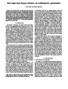
SVM results for hypothyroid 99,0

Classifier Accuracy [%]

98,5 98,0 97,5 97,0 SSV parts 16-32 SSV bfs SSV beam SBL ranking Mutual Information Ba 0.5

96,5 96,0 95,5 95,0

1 2 3 4 5 6 7 8 9 10 11 12 13 14 15 16 17 18 19 20 21

No. features

Fig. 2. Hypothyroid data, results obtained on subsets of features created by 4 methods

have been averaged over 10 runs), but that does not change the overall character of curve in Fig. 2. The best kNN result (k=4, Canberra) is achieved with 5 features, 17,3,8,19,21, reaching 98.75% on the test set, significantly higher than 97.58% with all features. This seems to be the best kNN result achieved so far on this dataset.

5 Conclusions Over 20 feature ranking methods based on information theory, correlation and purity indices have have been implemented and using hashing techniques applied also to feature selection with greedy search. Only a few results for artificial and real data have been presented here due to the lack of space. Several conclusions may be drawn from this and our more extensive studies: – The actual feature evaluation index (information, purity or correlation) may not be so important, therefore the least expensive indices (purity indices) should be used. – Discretization is very important; naive equi-width or equi-distance discretization may give unpredictable results; entropy-based discretization is etter but more costly, with the separability-based discretization offering less expensive. – Selection requires calculation of multidimensional evaluation indices, done effectively using hashing techniques. – Continuous kernel-based approximations to calculation of feature relevance indices are a useful, although little explored, alternative. – Ranking is easy if global evaluation of feature relevance is sufficient, but different sets of features may be important for separation of different classes, and some are important in small regions only (cf. decision trees), therefore results on Gaussian distributions may not reflect real life problems. – Local selection and ranking is the most promising technique.

Many open questions remain: discretization method deserve more extensive comparison, fuzzy partitioning may be quite useful, ranking indices may be used for feature weighting, not only selection, selection methods should be used to find combination of features that contain more information.

References 1. Liu H, Motoda H. (1998) Feature Extraction, Construction and Selection: A Data Mining Perspective. Kluwer Academic Publishers. 2. Liu H, Motoda H. (1998) Feature Selection for Knowledge Discovery and Data Mining. Kluwer Academic Publishers. 3. Duch W, Adamczak R. and Grabczewski ˛ K. (2001) Methodology of extraction, optimization and application of crisp and fuzzy logical rules. IEEE Transactions on Neural Networks 12: 277-306 4. Quinlan J.R. (1993) C4.5: Programs for machine learning. San Mateo, Morgan Kaufman 5. Breiman, L., Friedman, J. H., Olshen, R. A., and Stone, C. J. (1984). Classification and Regression Trees. Wadsworth and Brooks, Monterey, CA. 6. Kass, G.V. (1980). An exploratory technique for investigating large quantities of categorical data. Applied Statistics 29:119 – 127. 7. de Mantaras L.R. (1991) A distance-based attribute selection measure for decision tree induction. Machine Learning 6, 81-92. 8. Sridhar D.V, Bartlett E.B, Seagrave R.C. (1998) Information theoretic subset selection. Computers in Chemical Engineering 22, 613-626. 9. Battiti R. (1991) Using mutual information for selecting features in supervised neural net learning. IEEE Transaction on Neural Networks 5, 537-550. 10. Hall M.A. (1998) Correlation based feature selection for machine learning. PhD thesis, Dept. of Comp. Science, Univ. of Waikato, Hamilton, New Zealand. 11. Lorenzo J, Hernández M. and Méndez J. (1998) GD: A Measure Based on Information Theory for Attribute Selection. Lecture Notes in Artificial Intelligence 1484:124-135. 12. Duch W, Winiarski T, Grabczewski ˛ K, Biesiada J, Kachel, A. (2002) Feature selection based on information theory, consistency and separability indices. Int. Conf. on Neural Information Processing (ICONIP), Singapore, Vol. IV, pp. 1951-1955. 13. Grabczewski ˛ K, Duch W (2000) The Separability of Split Value Criterion, 5th Conf. on Neural Networks and Soft Computing, Zakopane, Poland, pp. 201-208. 14. C.L. Blake, C.J. Merz, UCI Repository of machine learning databases (2001) http://www.ics.uci.edu/ mlearn/MLRepository.html. 15. Duch W, Grudzi´nski K. (1999) The weighted k-NN method with selection of features and its neural realization. 4th Conf. on Neural Networks and Their Applications, Zakopane, May 1999, pp. 191-196. 16. Duch W, Diercksen G.H.F, Feature Space Mapping as a universal adaptive system, Computer Physics Communications 87, 341–371 (1995)