Feature Selection of Interval Valued Data through Interval K-Means Clustering D S Guru, N Vinay Kumar*, and Mahamad Suhil Department of Studies in Computer Science, University of Mysore, Manasagangotri, Mysore-570006, Karnataka, INDIA
[email protected],
[email protected],
[email protected]
ABSTRACT This paper introduces a novel feature selection model for supervised interval valued data based on interval K-Means clustering. The proposed model explores two kinds of feature selection through feature clustering viz., class independent feature selection and class dependent feature selection. The former one clusters the features spread across all the samples belonging to all the classes, whereas the latter one clusters the features spread across only the samples belonging to the respective classes. Here, these two kinds of feature selection are demonstrated to explore the generosity of clustering in selecting the interval valued features. For clustering, the kernel of the K-means clustering has been altered to operate on interval valued data. For experimentation purpose four standard benchmarking datasets and three symbolic classifiers have been used. To corroborate the effectiveness of the proposed model, a comparative analysis against the state-ofthe-art models is given and results show the superiority of the proposed model. Keywords: Feature selection, Interval data, Symbolic similarity measure, Symbolic classification, Interval K-Means Clustering INTRODUCTION In the current era of digital technology- pattern recognition plays a vital role in the development of cognition based systems. These systems quite naturally handle a huge amount of data. While handling such vast amount of data, the task of data processing has become curse to process. To overcome curse in data processing, the concept of feature selection is being adopted by researchers. Nowadays, feature selection has become a very demanding topic in the field of machine learning and pattern recognition, as it select the most relevant and non-redundant feature subset from a given set of features using a feature selection technique. Basically, the feature selection techniques are broadly classified into: filter, wrapper, and embedded methods (Artur et. al., 2012). Generally, the existing conventional feature selection methods (Artur et. al., 2012) fail to perform feature selection on unconventional data like interval, multi-valued, modal, and categorical data. These data are also called in general symbolic data. The notion of symbolic data was emerged in the early 2000, which mainly concentrates in handling very realistic type of data for effective classification, clustering, and even regression for that matter (Lynne and Edwin, 2007). As it is a powerful tool in solving problems in a natural way, we thought of developing a feature selection model for any one of the modalities. In this regard, we have chosen with an interval valued data, due its strong nature in preserving the continuous streaming data in discrete form (Lynne and Edwin, 2007). Thus, we built a feature selection model for interval valued data in this work. 1|Page
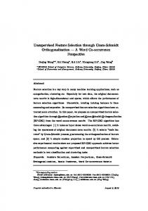
Initially, Manabu Ichino (1994) provided the theoretical interpretation of feature selection on interval valued data. The method works based on the pretended simplicity algorithm handled in Cartesian space. Later, there are couple of attempts found on feature selection done on mixed type data (i.e., interval, multi-valued, and qualitative). Bapu et. al., (2007) proposed a two stage feature selection algorithm which can handle both interval as well multi-valued data using Mutual Similarity Value proximity measure for un-supervised data. Qin et al., (2014) proposed an approach based on information theory which selects an optimal feature subset by computing modified heuristic mutual information. This approach handles both numeric and interval valued features. Lyamine et al., (2015) proposed a feature selection model which handles heterogeneous type data viz., interval, quantitative, and qualitative. The proposed feature selection model makes use of similarity margin and weighting scheme for selecting features. In addition to this the model converts the different types of data into a common type and further a common weighting scheme is employed on it. Lyamine et. al., (2011) present the feature selection of interval valued data based on the concept of similarity margin computed between an interval sample and a class prototype. The similarity margin is computed using a symbolic similarity measure. The authors have constructed basis for the similarity margin and then they worked out at the multi-variate weighting scheme. The weight corresponding to each feature decides the relevancy of that feature. Hence, they considered Lagrange Multiplier for optimizing the weights which results with the optimal set of features. The experimentation is done on three standard benchmarking interval dataset and validated using LAMDA classifier. Chih-Ching et. al., (2014) have come up with the model which make use (Lyamine et. al., 2011) in all aspects in selecting the features but with respect to similarity measure computation, the authors have used robust Gaussian kernel. The authors also have given an experimentation and a comparative analysis on only one interval dataset. Jian et al., (2016) proposed a heuristic approach for attribute reduction. This approach makes use of rough set and information theory for attribute reduction. In the theory of rough sets, if the efficiency of the optimal subset equals to the efficiency of original feature set then such process is termed as attribute reduction (instead of feature selection). Guru and Vinay (2016) proposed a feature selection model based on two novel feature ranking criteria for interval valued data. This model makes use of vertex transformation technique before computing the rank of the features. The ranked features are then sorted based on their relevancy before get selected through experimentation. The limitation of this model is the computation of vertex transformation for higher dimensional data which leads to exponential time complexity. Apart from the above mentioned works, no work can be seen on feature selection of interval valued data based on clustering of features. Clustering of features and then selecting the cluster representatives helps in improving the prediction accuracy. In addition, it also eliminates the redundant features, as it selects features which are of most relevant (Qinbao et. al., 2013). With this background, here in this paper, a feature selection model is proposed. The proposed feature selection model is based on clustering the interval features through interval K-Means clustering algorithm. The conventional K-Means clustering is modified to adopt the interval valued data by altering the conventional kernel with the symbolic interval similarity measures. The clustering of interval features for feature selection is realized in two different ways viz., class independent features clustering and class dependent features clustering. In the former approach, initially the supervised interval feature matrix (Figure 1(a)) is transformed and then the transformed feature matrix (Figure 1(b)) is fed into interval K-means clustering algorithm. Thus, results with the K clusters. Further, for each cluster, a cluster representative is 2|Page
computed that results with the K number of representatives corresponding to each cluster. These cluster representatives are then preserved in the knowledgebase as optimal features subset indices. During testing, a single interval feature vector is considered for classification based on the feature indices selected from the knowledgebase and they are validated using suitable symbolic classifiers. Henceforth, this approach is labelled as Class Independent Feature Selection (ClIFS) through interval K-means clustering. In the latter approach, initially the supervised interval feature matrix is transformed and later divides the transformed matrix into several (equal to number of classes) interval feature sub-matrices (Figure 1(b)). The transformed feature sub-matrices are then fed into interval K-means clustering algorithm. Thus, results with K clusters for each sub-matrix. Next, for every cluster, a cluster representative is computed that results with K number of representatives corresponding to each class. During testing, a single interval feature vector is considered for classification based on the class specific features selected from the knowledgebase and they are validated using suitable symbolic classifiers. Henceforth, this approach is labelled as Class Dependent Feature Selection (ClDFS) through interval Kmeans clustering. The major contributions of this paper are as follows: 1. 2. 3. 4.
Proposal of a novel interval feature selection model based on interval feature clustering. Two different ways of clustering is explored for interval valued feature selection. Conduction of extensive experiments on four benchmarking datasets. Comparative study of the proposed model against the state-of-the art models.
The organization of the paper is as follows: The proposed model is described in next section. The details of experimental setup, datasets, results and comparative analysis are given in subsequent sections. Finally, conclusion has been brought out in the last section.
(a)
3|Page
(b)
(c)
Figure 1. (a) Supervised Interval Valued Feature Matrix, (b) Transformed Interval Feature Matrix (ClIFS), (c) Transformed Interval Feature Matrix (ClDFS).
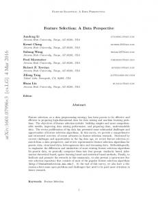
PROPOSED MODEL The proposed interval feature selection model is generalized for both class independent feature selection through clustering and class dependent feature selection through clustering. The model comprises of various stages in both training and testing respectively. Pre-processing, Interval KMeans clustering, selection of cluster representatives (Feature Selection) are done at the training phase and selection of feature indices (pre-processing), and classification tasks are performed at the testing phase. The generalized architecture of the proposed model is given in Figure 2.
Figure 2. General Architecture of the Proposed Model
4|Page
Pre-processing during training phase Let us consider a supervised interval valued feature matrix say IFM, with N number of rows and d+1 number of columns. Each row corresponds to a sample and each column corresponds to a feature of type interval and it is represented by: IFM: i , yi , where i represents a sample and yi represents a class label ( i 1, 2,..., N ) (Figure 1(a)).
Each sample i is described by d interval features and is given by:
i i1 , i2 ,..., id f1 , f1 , f 2 , f 2 ,..., f d , f d
where, f k and f k are the lower and upper limits of an interval respectively. The basic idea of the proposed model is to cluster the similar set of features. To accomplish this, a feature matrix should be transformed in such a way that the positions of samples become features and features become samples. That is, the rows of a feature matrix should correspond to features and the columns should correspond to samples. After matrix transformation, we have a transposed feature matrix TIFM of dimension d x N (ignores class labels). As we discussed earlier, the clustering of features can be done in two different ways (viz., class independent features and class dependent features) such that the behavior of the transformed feature matrix also changes accordingly. In the former case, the transformed feature matrix say TIFM of dimension d x N is directly fed into interval K-Means clustering algorithm to obtain K clusters from the transformed matrix, where d features are spread across K different clusters. Where as in the latter case, we separate the samples based on their class correspondence and obtained with a sub-matrix TIFM j of dimension d x n j ( n j is the number of samples per class) corresponding to a class C j j 1, 2,..., m; m no. of classes and is fed into interval K-Means clustering algorithm to obtain K clusters from each matrix, where d features are spread across mxK different clusters. In general, we represent the dimension of the transposed interval feature matrix TIFM as d x , where is a set consisting of N and n j ( n j is the number of samples per class) subsets. The details of clustering procedure are given in next section. Interval K-Means Clustering In this section, details about the construction of an interval K-Means clustering algorithm are given. As we know, conventional K-Means clustering is an instance of partitional clustering techniques. Initially, it fixes up with the number of clusters (K) and the centroid points. Then the algorithm uses one of the different kernels such as squared Euclidean/ city block/ cosine/ correlation/ Hamming distance to compute the proximity among the samples (Anil and Richard, 1988). Later those samples which have greater affinity go to same cluster and samples with a little affinity go to different clusters. Then the new centroids will be computed for each K clusters. The same procedure is repeated until certain convergence criteria are satisfied. The convergence criteria may be the maximum iterations or difference. Usually, the above said procedures are followed 5|Page
in conventional K-Means clustering algorithm. But, in our work, as we are handling with interval valued data, a slight modification has been brought out at kernel level. The kernel used to compute the affinity among the samples is symbolic similarity measure (Guru et. al., 2004) instead of the above said kernels. The symbolic similarity kernel (SSK) used in our work is given by: ISVAB ISVAB ISVBA ISVBA (1) SSK A, B 4
Where A a1 , a1 , a2 , a2 ,..., ak , ak ,... and B b1 , b1 , b2 , b2 ,..., bk , bk ,... be two
interval objects. ISVAB be the lower and upper limits of interval similarity , ISVAB ISVBA , ISVBA
value computed from object A to object B (B to A) and are given by: ISVAB min Sim Ak , Bk ; k 1, 2,..., d ISVAB max Sim Ak , Bk ; k 1, 2,..., d
ISV A, B ISV , ISV 1 Length of overlapping portion of Aand B Sim Ak , Bk Length of B 0 A 𝑎1− B
𝑏2−
A
𝑎1−
𝑎1+
𝑏2−
𝑏2+
𝑎1−
A
𝑎1−
𝑎1+
B
A
(d)
B
𝑏2+
𝑏2−
(c) 𝑎1−
𝑏2−
(e)
𝑎1+
𝑏2+ A
𝑎1+
B
B 𝑏2+
A
𝑎1−
𝑎1+
B 𝑏2−
𝑎1+
(b)
(a)
if Acontains B if there exists overlapping if thereis no overlapping
𝑏2+
𝑏2−
𝑏2+ (f)
Figure 3. Different instances of similarity computation between two intervals (Bapu et. al., 2007), (a)-(d): Overlapping cases, (e)-(f): Non-overlapping cases
The symbolic similarity kernel used in this work is very realistic in nature, as it preserves the topological relationship between the two intervals. The illustration of different cases of topological relationships exist between two intervals are shown in Figure 3. The rest of the interval K-Means clustering follows the same procedure as conventional KMeans clustering as explained above.
6|Page
Selection of Cluster Representative (Feature Selection) In this section, the details of cluster representative selection are given. The cluster representatives are selected based on the type of a matrix with which the clustering algorithm performed clustering. If the algorithm is applied with ClIFS case, then the clustering algorithm results with K-clusters independent of classes Call . If it in case of ClDFS , the clustering algorithm results with K-clusters from each class C j j 1, 2,..., m; m no. of classes resulting with mxK clusters. In general, these clusters are represented as clusters, where is a set which includes { K } and {mxK} as subsets and classes are represented as C , where set C includes Call and C j as its subsets.
The procedure for selecting the cluster representatives is discussed below: Consider a cluster Clq C , containing z number of features. A feature is said to be a cluster
representative ClRq , then it must exhibit a maximum similarity to all the remaining features. In this regard, the similarity computation among the features in a cluster Clq results with a similarity matrix SM q , which is given by: q SM ab SSK Fa , Fb , a 1, 2,..., z; b 1, 2,..., z
Where, SSK Fa , Fb is given by equation (1).
Further, the computation of average similarity value is given by: 1 z q (2) ASVa SM ab z b 1 Now, we have obtained with average similarity values corresponding to cluster Clq . Thus ClRq is given by:
ClRq arg max Fa
ASV , ASV ,..., ASV '
1
2
z
' z 1 z 1 z q 1 q q i.e., ClRq arg max SM 1b , SM 2b ,..., SM zb z b 1 z b 1 Fa z b 1
(3)
The feature ( Fa ) which gives maximum ASVa value is considered as a cluster representative ClRq corresponding to cluster Clq . Thus the above procedure is repeated for all the clusters
corresponding to remaining classes of set C . Now we have K such clusters representative ' ClIFS and mxK such clusters representative ClR1 , ClR2 ,..., ClRK in case of ' ClR1 , ClR2 ,..., ClRmK in case of ClDFS . The feature indices of these cluster representatives are further used to select features from original interval feature matrices and archived the same in the knowledgebase for classification. The illustration of selection of cluster representatives (features selection) is shown in Figure 4.
7|Page
(a)
(b)
(c)
(d)
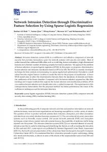
Figure 4: Illustration of interval features selection using clustering (Guru and Vinay, 2016(b)): (a) Interval features (visualized as points) are spread in two dimensional sample space, (b) Clusters obtained after applying interval KMeans clustering, (c) Red dots are the clusters representative selected based on the procedure explained in the above section, (d) Two red dots are further retained as the features of interest.
Pre-processing during testing phase In this work, we have shown two types clustering, even here, the procedure for choosing a test sample varies from one method to other method. In case of ClIFS , an unknown test sample is taken from a pool of test samples and the (K) feature indices of the test sample are selected based on the corresponding (K) feature indices which are preserved at the training stage. Thus for classification, there is only one query sample entering into the symbolic classifier. In case of ClDFS , a query sample is claimed as not only the member of a single class instead it is claimed to be as the member of all m different classes. While claiming the membership of all m classes, the K features of a query sample are selected based on the feature indices preserved during training. Thus for classification, there are totally m different query instances (of a sample) entering into the symbolic classifier. Symbolic Classifiers In this paper, as we are handling with interval type data, it is difficult to compatible with conventional classifiers such as K-NN, SVM, Random Forest, Naïve Bayesian etc., (Duda et. al., 2000). Hence, symbolic classifiers are recommended to handle interval valued data for classification (Bapu, 2006), (Guru and Nagendraswamy, 2006). Here, we use three different symbolic classifiers proposed in (Bapu, 2006), (Guru and Nagendraswamy, 2006) and (Hedjazi et. al., 2006). Henceforth, these three are called as C-1, C-2, and C-3 classifiers respectively. The classifier proposed in (Bapu, 2006), operates directly on interval data and the similarity measure proposed by them is of interval type in nature, hence the computed similarity matrix is again a symbolic. Further, authors aggregate the obtained matrix using the concept of mutual similarity value (MSV) and obtain with the conventional symmetric similarity matrix. Later on, the authors follow the nearest neighbour approach for classification. In (Guru and Nagendraswamy, 2006), authors propose a symbolic classifier which mainly concentrates on nearest neighbour approach in classifying an unknown sample to a known class. In our work, a slight modification has been done on the similarity measure proposed by (Guru and Nagendraswamy, 2006). The slight modification of the above said similarity measure is done at feature level. As the similarity measure in (Guru and Nagendraswamy, 2006), is capable of measuring the similarity of multi-interval valued data, but in our case, only single interval valued 8|Page
data is enough to measure the similarity between two objects. Hence, we have restricted the measure to only single interval valued data. Hedjazi et al., (2009) designed a symbolic classifier termed as LAMDA classifier which works based on the estimation of similarity between two intervals using similarity kernel. The proposed classifier makes use of fuzzy mixed type approach for classification. Classification To classify an unknown sample, any of the symbolic classifiers discussed in the above section is adopted. The symbolic classifier results with many classification scores corresponding to the sample used for classification. Further these classification scores are used in deciding the class of the sample. Here, the decision making procedure varies with respect to the two different cases of the proposed feature selection model. Let us consider an interval test sample ISt to be classified as a member of any one of the existing classes. In case of ClIFS , the classification scores are given by:
CSall SC RS , ISt Where,
SC . is any symbolic classifier,
RS corresponds to all
reference samples
RS rs1 rs2 ... rsm .
Here, we end up with N different classification scores CSall obtained from comparing the
unknown sample with N different reference samples RS . These classification scores play a vital role in labeling the unknown sample into a label sample. A class which possesses a maximum classification score is given as the class membership of the unknown sample. In case of ClDFS , the classification scores are given by: CS j Avg SC rs j , ISt
Where, rs j is a set of reference samples belongs to class C j .
Here, we obtained with m different classification scores CS j ; j 1, 2,..., m from m different classes. The classification of the unknown sample is labelled based on these scores. A class which possesses a maximum classification score is given as the class membership for the unknown sample. In general, the classification scores CS all and CS j are treated as subsets of a set CS . EXPERIMENTATION AND RESULTS Datasets We have used totally four different supervised interval datasets for experimentation. The four different benchmarking datasets used are: Iris (Lynne and Edwin, 2007), Car (Carvalho et. al., 2006), Water (Quevedo et. al., 2010), and Fish (Carvalho et. al., 2006) datasets. The Iris interval dataset consists of 30 samples with 4 interval features. The 30 samples are spread across the 9|Page
three different classes, with 10 samples per class. The Car dataset consists of 33 samples with 8 interval features. The samples are spread across the four different classes with 10, 8, 8, and 7 samples per class respectively. The Fish dataset consists of 12 samples with 13 interval features. The samples are spread across four different classes, each with 4, 2, 4, and 2 samples respectively. Finally, the Water dataset consists of 316 samples with 48 interval features. The samples are spread across 2 different classes, each with 223 and 93 samples respectively. Among four datasets, the fish dataset seems to provide very less instances for classification. Thus for this dataset, the classification results vary a lot compare to other datasets. Experimental Setup In this sub-section, details of experimentation conducted on the four benchmarking supervised interval datasets are given. The experimentation is conducted in two phases viz., training, and testing. During training phase, we consider a supervised interval feature matrix and obtained the class independent or class specific features depending on the chosen technique as explained in pre-processing during training phase section. These features are then preserved in a knowledgebase for classification. During testing phase, an unknown interval sample is considered and selected its class independent or class specific features and performed classification as explained in classification section. During training and testing, the samples of the dataset are varied from 30 percent to 70 percent (in steps 10 percent) and 70 percent to 30 percent (in steps 10 percent) respectively. For, interval K-Means clustering the maximum number of iterations is fixed to be 100. The value of K in interval K-Means clustering is varied from 2 to one less than number of features for all datasets except water dataset (In case of water dataset, the K is varied till 21, as the clustering algorithm does not converge above that value). The parameter β in the symbolic classifier (C-2) is fixed to be 1. Results The validation of the proposed feature selection model is performed using classification accuracy, defined as the ratio of correctly classified samples to the number of samples. The experimental results are tabulated for the best feature subset (results with feature selection (WFS)) obtained from the corresponding train-test percentage of samples and also we have compared the classification results of the same datasets without using any feature selection methods (results without feature selection (WoFS)). The results with respect to ClIFS are given from Table 1 to Table 4 and ClDFS are given from Table 5 to Table 8 respectively.
10 | P a g e
TrainTest
# of Features
Accuracy
# of Features
Accuracy
# of Features
Accuracy
# of Features
Accuracy
# of Features
Accuracy
# of Features
Accuracy
Table-1: Comparison of classification accuracies obtained from the classifiers C-1, C-2, and C-3 with different training-testing percentage for Iris dataset (ClIFS) C-3 C-1 C-2 WFS WoFS WFS WoFS WFS WoFS
30-70 40-60 50-50 60-40 70-30 80-20
2 3 3 2 2 2
100 100 100 100 100 100
4 4 4 4 4 4
100 100 100 91.67 88.89 100
2 3 3 2 3 3
100 100 100 100 100 100
4 4 4 4 4 4
100 100 100 100 100 100
2 3 2 2 2 2
100 100 100 100 100 100
4 4 4 4 4 4
95.24 94.44 93.33 91.67 100 100
TrainTest
# of Features
Accuracy
# of Features
Accuracy
# of Features
Accuracy
# of Features
Accuracy
# of Features
Accuracy
# of Features
Accuracy
Table-2: Comparison of classification accuracies obtained from the classifiers C-1, C-2, and C-3 with different training-testing percentage for Car dataset (ClIFS) C-3 C-1 C-2 WFS WoFS WFS WoFS WFS WoFS
30-70 40-60 50-50 60-40 70-30 80-20
3 5 4 2 2 2
61.90 66.67 62.5 66.67 66.67 80
8 8 8 8 8 8
42.86 38.89 50 50 55.56 60
6 3 6 7 6 2
80.95 83.33 87.50 91.67 100 100
8 8 8 8 8 8
71.43 77.78 81.25 83.33 88.89 80
2 4 4 3 3 3
80.95 77.78 68.75 83.33 77.78 80
8 8 8 8 8 8
47.62 61.11 56.25 58.33 66.67 80
TrainTest
# of Features
Accuracy
# of Features
Accuracy
# of Features
Accuracy
# of Features
Accuracy
# of Features
Accuracy
# of Features
Accuracy
Table-3: Comparison of classification accuracies obtained from the classifiers C-1, C-2, and C-3 with different training-testing percentage for Fish dataset (ClIFS) C-3 C-1 C-2 WFS WoFS WFS WoFS WFS WoFS
30-70 40-60 50-50 60-40 70-30
3 7 2 2 2
83.33 83.33 66.67 50 100
13 13 13 13 13
100 100 100 91.67 88.89
3 7 2 3 8
100 50 83.33 100 100
13 13 13 13 13
66.67 66.67 66.67 100 100
8 2 6 4 2
66.67 66.67 66.67 100 100
13 13 13 13 13
16.67 16.67 16.67 50 50
11 | P a g e
TrainTest
# of Features
Accuracy
# of Features
Accuracy
# of Features
Accuracy
# of Features
Accuracy
# of Features
Accuracy
# of Features
Accuracy
Table-4: Comparison of classification accuracies obtained from the classifiers C-1, C-2, and C-3 with different training-testing percentage for Water dataset (ClIFS) C-3 C-1 C-2 WFS WoFS WFS WoFS WFS WoFS
30-70 40-60 50-50 60-40 70-30 80-20
11 15 12 16 6 2
70.59 71.28 70.70 70.63 70.97 74.19
48 48 48 48 48 48
66.52 65.96 65.61 54.76 63.44 72.58
2 3 4 7 10 15
70.14 68.09 71.34 74.60 74.19 77.42
48 48 48 48 48 48
63.80 60.11 56.05 62.70 59.14 70.96
13 9 12 14 11 5
68.33 68.09 67.52 73.02 73.12 72.58
48 48 48 48 48 48
63.80 60.11 56.05 62.70 59.14 70.96
TrainTest
# of Features
Accuracy
# of Features
Accuracy
# of Features
Accuracy
# of Features
Accuracy
# of Features
Accuracy
# of Features
Accuracy
Table-5: Comparison of classification accuracies obtained from the classifiers C-1, C-2, and C-3 with different training-testing percentage for Iris dataset (ClDFS) C-3 C-1 C-2 WFS WoFS WFS WoFS WFS WoFS
30-70 40-60 50-50 60-40 70-30 80-20
3 2 2 2 2 2
100 100 100 100 100 100
4 4 4 4 4 4
100 100 100 91.67 88.89 100
3 2 3 2 3 2
100 100 100 100 100 100
4 4 4 4 4 4
100 100 100 100 100 100
3 2 2 2 2 2
100 100 100 100 100 100
4 4 4 4 4 4
95.24 94.44 93.33 91.67 100 100
TrainTest
# of Features
Accuracy
# of Features
Accuracy
# of Features
Accuracy
# of Features
Accuracy
# of Features
Accuracy
# of Features
Accuracy
Table-6: Comparison of classification accuracies obtained from the classifiers C-1, C-2, and C-3 with different training-testing percentage for Car dataset (ClDFS) C-3 C-1 C-2 WFS WoFS WFS WoFS WFS WoFS
30-70 40-60 50-50 60-40 70-30 80-20
2 4 3 2 7 6
76.19 72.22 81.25 66.67 75.27 79.03
8 8 8 8 8 8
42.86 38.89 50 50 55.56 60
5 4 6 4 2 2
76.47 61.11 71.97 83.33 77.42 70.97
8 8 8 8 8 8
71.43 77.78 81.25 83.33 88.89 80
6 2 6 4 5 4
70.59 72.22 68.79 83.33 67.74 75.81
8 8 8 8 8 8
47.62 61.11 56.25 58.33 66.67 80
12 | P a g e
TrainTest
# of Features
Accuracy
# of Features
Accuracy
# of Features
Accuracy
# of Features
Accuracy
# of Features
Accuracy
# of Features
Accuracy
Table-7: Comparison of classification accuracies obtained from the classifiers C-1, C-2, and C-3 with different training-testing percentage for Fish dataset (ClDFS) C-3 C-1 C-2 WFS WoFS WFS WoFS WFS WoFS
30-70 40-60 50-50 60-40 70-30
3 5 10 3 8
66.67 100 66.67 100 100
13 13 13 13 13
66.67 66.67 66.67 100 100
6 7 10 2 2
50 66.67 66.67 50 50
13 13 13 13 13
66.67 66.67 66.67 100 100
3 9 4 5 5
66.67 83.33 66.67 100 100
13 13 13 13 13
16.67 16.67 16.67 50 50
TrainTest
# of Features
Accuracy
# of Features
Accuracy
# of Features
Accuracy
# of Features
Accuracy
# of Features
Accuracy
# of Features
Accuracy
Table-8: Comparison of classification accuracies obtained from the classifiers C-1, C-2, and C-3 with different training-testing percentage for Water dataset (ClDFS) C-3 C-1 C-2 WFS WoFS WFS WoFS WFS WoFS
30-70 40-60 50-50 60-40 70-30 80-20
11 14 5 4 2 4
68.78 68.09 70.70 69.84 76.34 79.03
48 48 48 48 48 48
66.52 65.96 65.61 54.76 63.44 72.58
2 14 6 20 10 17
71.50 71.81 73.89 77.78 79.57 79.03
48 48 48 48 48 48
63.80 60.11 56.05 62.70 59.14 72.58
4 4 6 10 6 2
69.68 70.21 68.79 70.63 74.19 75.81
48 48 48 48 48 48
63.80 60.11 56.05 62.70 59.14 70.96
From the above tables (Table 1 to 8), it is very clear that the classification performance has been increased due to the incorporation of feature selection method compared to that of not using any feature selection method. It is also so clear that the best results are quoted for lesser number of features. In addition to this, the best results obtained from the three different classifiers with varied training and testing samples corresponding to ClIFS and ClDFS are given in Figure 5 (a)(d) and Figure 5 (e) to 5 (h) respectively. From the figure, one can observe that the former method gives better results for smaller dimensional feature dimensions when compared to the latter one which performs better on higher dimensional feature dimensions. The results obtained from the three classifiers are almost similar for all datasets except Fish dataset, where the results are varied with the different classifiers used. This is because the sample size of the Fish dataset is much smaller when compared to the number of features. To test effectiveness of the proposed model, we have used the datasets containing different feature dimensions (from 4 to 48). From the results, one can notice that the model performs well even for such kind of datasets in-spite of selecting very few features. This shows the robustness of the proposed model under varied feature sizes of the dataset.
13 | P a g e
(a)
(b)
(c)
(d)
(e)
(f)
(g)
(h)
Figure 5: (a)-(d) represent accuracy obtained from the three different classifiers (C-1, C-2, and C-3) on different datasets with respect to ClIFS; (e)-(h) represent accuracy obtained from the three different classifiers (C-1, C-2, and C-3) on different datasets with respect to ClDFS.
COMPARATIVE ANALYSIS To corroborate the effectiveness of the proposed model, the comparative analyses are given. Initially, the proposed model is compared against the state-of-the-art methods in terms of classification accuracy and the same is tabulated in Table 9. Further, we have compared our model with the other models which do not use any feature selection during classification. In literature, we found such classification models reported only on Car dataset. Hence, we have given comparison with only Car dataset and is given in Table 10.
14 | P a g e
Table-9: Comparison of proposed feature selection method v/s other existing methods
Methods
Classifier
C-1 C-2 C-3 Proposed C-1 ClDFS C-2 C-3 Lyamine et. al., 2011 LAMDA Chih-Ching et. al., 2014 LAMDA Qin Liu et al., 2014 KNN KNN RBD PNN KNN IU PNN Jian-hua et al., 2016 KNN PD PNN KNN UMAR PNN C-1 CCS C-2 Guru and Vinay, 2016(a) C-1 CSS C-2 ClIFS
IRIS dataset 100 (2) 100 (2) 100 (2) 100 (2) 100 (2) 100 (2) -----------100 (1) 100 (2) 100 (1) 100 (1)
Accuracy (Feature Subset) CAR FISH dataset dataset 80 (2) 100 (2) 100 (3) 100 (2) 83.33 (3) 100 (4) 81.25 (3) 100 (3) 83.33 (4) 66.67 (7) 83.33 (4) 100 (5) 78 (5) 74 (4) --80 (6) 75 (7) 81.2 (6) 58.33 (8) 81.2 (6) 75 (8) 72.73 (6) 66.67 (10) 69.7 (6) 66.67 (10) 63.64 (7) 66.67 (9) 63.64 (7) 66.67 (9) 69.7 (7) 58.33 (12) 72.73 (7) 58.33 (12) 77.78 (2) 100 (3) 87.50 (3) 66.67 (6) 83.33 (2) 50 (1) 91.67 (5) 50 (1)
WATER dataset 74.19 (2) 77.42 (15)
73.12 (11) 79.03 (4) 79.57 (10) 75.81 (2)
77 (14) 78.66 (11) 78 (27) -------------
From Table 9, it is very clear the proposed feature selection model outperforms the state-of-the art models found in the literature both in terms of accuracy and also in terms of feature subset selection. Though, (Guru and Vinay, 2016) gives good results for lower dimensional features, which uses vertex transformation based approach, but it has some limitations in handling higher dimensional features. This reflects in the absence of results corresponding to Water dataset (48 features) in Table 9. The selected feature subset indices of the best results (class independent features and class specific features) obtained from the classifiers C-1, C-2 and C-3 are given in Table 11 and Table12 respectively. With respect to Table 11, the numbers within the curly braces represent the class independent feature indices of the best results obtained from three different classifiers. Similarly, with respect to Table 12, the numbers within the small braces represent the class dependent feature indices of the best results obtained from three different classifiers and the number of such small braces set within curly braces represents the number of classes.
15 | P a g e
Table-10: Comparison of classification with the proposed feature selection method v/s the existing classification methods without using any feature selection methods for Car interval dataset Methods C-1 (WFS) C-2 (WFS) C-3 (WFS) C-1 (WFS) C-2 (WFS) ClDFS C-3 (WFS) Binary Model Multinomial IDPC-CSP IDPC-VSP IDPC-PP Distributional approach Mid points and Ranges
ClIFS
Proposed Method
Barros et. al., 2012 Renata et. al., 2011 Silva and Bruto, 2006
Accuracy
80 (2) 100 (2) 83.33 (3) 81.25 (3) 83.33 (4) 83.33 (4) 48.49 (8) 54.55 (8) 63.64 (8) 63.6 (8) 72.8 (8) 73 (8) 55 (8)
Table-11: Selected feature subsets and their corresponding feature indices (ClIFS) C-1 C-2 C-3 {1,4} {1,4} {1,4} {1,3} {1,3} {1,5,6} {10,2} {5,13,7} {10,2} {24,41,29,34,16,30,21,44,27,23,47,2,13,18, Water {18,5} {27,9,5,48,44,22,35,20,39,18,33} 36}
Dataset Iris Car Fish
Table-12: Selected feature subsets and their corresponding feature indices (ClDFS) Dataset (# of Class) Iris (3) Car (4)
C-1
C-2
C-3
{(2,1),(1,4),(2,3)}
{(2,1),(1,4),(2,3)}
{(2,1),(1,4),(2,3)}
{(1,3,4), (2,4,1), (3,1,2), (1,8,4)}
{(4,3,6,1), (1,2,3,4), (2,1,5,4), (1,8,6,5)} {(1,9,3,12,2,4,7), (1,3,5,9,11,6,7), (9,11,1,5,8,6,12), (3,12,2,9,8,13,7)} {(38,42,18,8,34,35,40,24,4,14), (13,32,27,31,22,34,36,18,3,16)}
{(4,3,6,1), (1,3,2,4), (2,5,1,4), (1,8,6,5)}
Fish (4)
{(12,4,7), (8,1,9), (4,12,1), (9,3,6)}
Water (2)
{(5,18), (23,34)}
{(1,12,4,7,9),(13,4,1,5,8),(13,5,8,9,2) ,(13,7,3,12,1)} {(19,24),(35,7)}
CONCLUSION In this paper, a novel idea for selection of supervised interval data through clustering is introduced. The proposed model realizes the features clustering for interval features selection in two different ways viz., Class Independent Features Clustering and Class Dependent Features Clustering. For clustering, it incorporates the concept of symbolic similarity measure to build the interval K-Means clustering. The cluster representatives are computed based on the symbolic similarity measure. Later on, the indices of cluster representatives are preserved in the knowledgebase. During testing, for a sample, the feature indices (either class independent or class dependent) are selected from knowledgebase and classified using symbolic classifier. The 16 | P a g e
proposed model has been well exploited for different interval supervised datasets and also it outperformed against other existing models in terms of classification accuracy and also in terms of feature dimensions. ACKNOWLEDGEMENT The second author would like to acknowledge the Department of Science Technology, INDIA, for their financial support through DST-INSPIRE fellowship. The third author of this paper acknowledges the financial support rendered by the University of Mysore under UPE grants for the High Performance Computing laboratory. REFERENCES Anil K. Jain and Richard C. Dubes, (1988). Algorithms for Clustering Data. Prentice-Hall, Inc., Upper Saddle River, NJ, USA Artur J. Ferreira and Mário A.T. Figueiredo, (2012). Efficient feature selection filters for high-dimensional data, Pattern Recognition Letters 33, pp. 1794–1804. Bapu B. Kiranagi, (2006). Classification of Symbolic Data through Symbolic Similarity and Dissimilarity Measures, PhD Thesis, University of Mysore, Mysore. Bapu B. Kiranagi, D. S. Guru, Manabu Ichino, (2007). Exploitation of Multivalued Type Proximity for Symbolic Feature Selection, Proc. of the Internal Conf. on Computing: Theory and Applications, IEEE, pp. 320-324. Barros Alberto Pereira de, Francisco de Assis Ten´orio de Carvalho and Eufr´asio de Andrade Lima Neto, (2012). A Pattern Classifier for Interval-valued Data Based on Multinomial Logistic Regression Model, IEEE International Conference on Systems, Man, and Cybernetics, pp. 541-546. Carvalho de Franscisco A T, De Souza, R.M.C.R., Chavent, M., Lechevallier, Y., (2006). Adaptive Hausdorff distances and dynamic clustering of symbolic interval data. Pattern Recognition 27, 167–179. Chih-Ching Hsiao, Chen-Chia Chuang, and Shun-Feng Su, (2014). Robust Gaussian Kernel Based Approach for Feature Selection, Advances in Intelligent Systems and Computing 268, pp. 25-33. Duda O R, Hart E P, and Stork G D. (2000). Pattern classification, 2nd Edition, Wiley-Interscience. Guru D S and Vinay Kumar N, (2016(a)). Novel Feature Ranking Criteria for Interval Valued Feature Selection, IEEE International Conference on Advances in Computing, Communications and Informatics, pp. 149-155. Guru D S and Vinay Kumar N, (2016(b)). Class Specific Feature Selection of Interval Valued Data through Interval K-Means Clustering, Springer International Conference Recent Trends in Image Processing and Pattern Recognition (Accepted and Presented). Guru D. S. and Nagendraswamy H. S., (2006). Symbolic representation and classification of two- dimensional shapes, Proceedings of the 3rd Workshop on Computer Vision, Graphics, and Image Processing (WCVGIP), pp. 19-24.
17 | P a g e
Guru D. S., Bapu B. Kiranagi, and Nagabhushan P., (2004). Multivalued type proximity measure and concept of mutual similarity value useful for clustering symbolic patterns, Pattern Recognition Letters 25, pp. 1203–1213. Ichino Manabu, (1994). Feature Selection for Symbolic Data Classification, New Approaches in Classification and Data Analysis, Springer, section 2, pp. 423-429. Jian-hua DAI, Hu HU, Guo-jie ZHENG, Qing-hua HU, Hui-feng HAN, and Hong SHI, (2016). Attribute reduction in interval-valued information systems based on information entropies, Frontiers of Information Technology & Electronic Engineering, Vol. 17(9), pp. 919-928. Lyamine Hedjazi, Aguilar Martin J., Lann M. V. L., (2011). Similarity-Margin based Feature Selection for Symbolic Interval Data, Pattern Recognition Letters, vol. 32, pp. 578-585. Lynne Billard and Edwin Diday. (2007). Symbolic Data Analysis: Conceptual Statistics and Data Mining, John Wiley & Sons. Qin Liu, Jing Wang, Jiakai Xiao, Hongming Zhu, (2014). Mutual Information based Feature Selection for Symbolic Interval Data, Proc. of International Conference on Software Intelligence, Technologies and Applications, pp. 62-69. Qinbao Song, Jingjie Ni, and Guangtao Wang, (2013). A Fast Clustering-Based Feature Subset Selection Algorithm for High-Dimensional Data, IEEE Transactions on Knowledge and Data Engineering, Vol. 25, No. 1, pp. 1-14. Quevedo, J., Puig, V., Cembrano, G., Blanch, J., Aguilar, J., Saporta, D., Benito, G., Hedo, M., Molina, A., (2010). Validation and reconstruction of flow meter data in the Barcelona water distribution network. J. Control Eng. Practice 18, 640–651. Renata M. C. R. de Souza, Diego C. F. Queiroz, and Francisco Jose´ A. Cysneiros, (2011). Logistic regression-based pattern classifiers for symbolic interval data, Pattern Anal Applic 14, pp. 273–282. Silva Antdnio Pedro Duarte and Brito Paula, (2006). Linear Discriminant Analysis for Interval Data, Computational Statistics 21, pp. 289-308.
.
18 | P a g e