Korean J. Chem. Eng., 25(4), 646-655 (2008)
SHORT COMMUNICATION
Fed-batch optimization of recombinant α-amylase production by Bacillus subtilis using a modified Markov chain Monte Carlo technique Wanwisa Skolpap*,†, Somboon Nuchprayoon**, Jeno M. Scharer***, Nurak Grisdanurak*, Peter L. Douglas***, and Murray Moo-Young*** *Department of Chemical Engineering, Thammasat University, Pathumthani, 12120 Thailand **Department of Electrical Engineering, Chiang Mai University, Chiang Mai, 50200 Thailand ***Department of Chemical Engineering, University of Waterloo, Waterloo, N2L 3G1 Canada (Received 25 October 2007 • accepted 16 January 2008) Abstract−A modified Markov Chain Monte Carlo (MCMC) searching procedure was developed to search for an optimal set of decision variables and optimal feed rate trajectories for recombinant α-amylase expression by Bacillus subtilis ATCC 6051a. The bacterium also synthesizes proteases as undesirable products in fed-batch culture that need to be minimized. To maximize α-amylase productivity, a 14th-order fed-batch model was optimized by integrating Pontryagin’s maximum principle with the Luedeking-Piret equation. The number of iterations and simulations of the proposed searching procedure were statistically examined for accuracy and acceptability of the results. It can be concluded that the proposed searching procedure increased the parameter selection opportunity near the tail ends of redefined triangular distribution. By applying a modified MCMC searching procedure with 1,500 iterations, the predicted αamylase productivity was improved by 18% in comparison with near-optimum experimental results. This productivity was 3.5% higher than predicted by conventional MCMC optimization. Key words: Bacillus subtilis, Fed-batch Culture, Nonlinear Optimization Problem, Markov Chain Monte Carlo
INTRODUCTION
estimate model parameters and decision variables in 14th-order equations for α-amylase and protease producing Bacillus subtilis in fedbatch culture [11] and to estimate a set of decision variables for penicillin fed-batch optimization problem by using a set of initial values given by Mekarapiruk and Luus [9,12]. In fed-batch optimization, the parameters to be optimized are embedded in a set of nonlinear differential equations. The problem observed during previous applications of the MCMC optimization technique was that parameter selection for optimal solution was often near the mean parameter value of the prior distribution. To properly select parameter values near the tail ends of the parameter distribution and also solve a set of nonlinear differential equations, excessive computing time was required. In this work, selection opportunity could be enhanced and computing time could be reduced by redefining the parameter distribution after a finite number of trials. As a result, the optimal feed-rate profile for the dual-enzyme fedbatch culture of B. subtilis [11] was quickly obtained and was comparable to the results obtained by using conventional searching procedure.
Fed-batch culture offers advantages over batch processes such as minimized problems pertaining to substrate inhibition and/or catabolite repression. However, optimization of fed-batch processes is not an easy problem. The challenge of dynamic fed-batch optimization often involves the resolution of high-order, nonlinear and multimodal systems. In previous efforts, both stochastic and deterministic search techniques have been applied to maximize productivity. Evolutionary algorithms, such as genetic algorithms mimicking the principles of natural biological evolution [1-4], or ant colony algorithm mimicking food search of ants [5], have also been applied to solve for optimal feed-rate profiles. In addition to those population-based search techniques, many point-based search techniques have been also applied to determine optimal feed-rate profiles. For instance, Patkar et al. [6] successfully applied a first-order conjugate gradient algorithm for optimizing fed-batch fermentations. Cuthrell and Biegler [7] employed an orthogonal collocation-based sequential quadratic programming to optimize fed-batch culture for penicillin production (containing four state variables) that was first studied by Lim et al. [8]. Mekarapiruk and Luus [9] applied iterative dynamic programming with unspecified initial conditions to optimize feed-rate policy for producing penicillin. Their study evaluated the feed-rate profile together with the initial volume and initial substrate concentration. Three deterministic candidates given for the values of the decision variables with a fixed final time at 132 hours and equally step size were obtained from their previous work [10]. Markov Chain Monte Carlo (MCMC) procedures, the Gibbs parameter sampling and the Metropolis-Hasting algorithm, have been recently used to
THE FED-BATCH MODEL The fed-batch model represents the dynamic optimization system for α-amylase synthesis under nitrogen-limited growth of Bacillus subtilis ATCC 6051a [11]. Undesirable proteases were hypothesized to cause the degradation of α-amylases. The model includes mass balances of cell growth, substrate uptake, respiration, target products formation as well as byproduct (ethanol, acetate, and lactate) channeling into oxidative and overflow metabolism. Table 1 shows a list of 13 nonlinear differential equations used in this work, while the model equations are shown in Appendix A. The differential equation for the volume change as the function of the feed rate is as follows:
To whom correspondence should be addressed. E-mail:
[email protected]
†
646
Fed-batch optimization of recombinant α-amylase production by Bacillus subtilis using a modified MCMC technique
Table 1. List of 13 nonlinear differential equations used in fed-batch model (see Appendix A for details) Equation number
Description
A.10 A.20 A.30 A.40 A.50 A.60 A.70 A.80 A.90 A.10 A.11 A.12 A.13
Biomass concentration Ammonia concentration α-Amylase concentration α-Amylase activity Protease concentration Protease activity Ethanol concentration Lactate concentration Acetate concentration Citrate concentration Starch concentration Isoleucine concentration Threonine concentration
dV u = -------. dt
The dynamic nonlinear optimization problem consists of the fedbatch model equations listed in Table 1, the objective function stated in Eq. (4), and the control variable (feed rate) given in Eq. (5). ⎛ PV -------⎞ lim Maximize ⎝T⎠ u, K, t
( O − E )2 Eq
q
(2)
where Oq is an observation in the qth row of the same column, Eq is an expectation in the qth row of the same column, and Q is a number of data points in any column. df=Q−1
(4)
s
where u is substrate feed rate and V is culture volume. The time-dependent value of feed rate in Eq. (1) was simply derived from the proposed optimization algorithm. It should be emphasized that α-amylase synthesis was proven to be partially growth associated and the relationship between enzyme production and growth was modeled successfully by the well-known Luedeking-Piret equation [13]. Due to proteolytic effect on α-amylase, the conversion from α-amylase concentration to activity was necessary for simulations. The time-averaged productivity of αamylase was maximized by integration of Pontryagin’s maximum principle and comparison with observed data, i.e., relationship between modeled product and cell growth and experimental results [11]. The set of nonlinear differential equations was solved by using the orthogonal collocation method encoded in MATLAB¨ (the MathWorks, Inc., Natick, MA) by Constantinides and Mostoufi [14]. Prior to optimization the fed batch model needed to be validated by using the experimental results [11,15]. The goodness of fit was evaluated non-parametrically by employing χ 2 statistical method [16]. It signifies the quality of agreement between predicted and observed results. The χ 2 statistic is calculated as follows: Q
where df is a degree of freedom. The five state variables for statistical analysis included the biomass concentration (y1), ammonia concentration (y2), α-amylase activity (y4), protease activity (y6), and starch concentration (y11). The results are summarized in Table 2. According to χ 2 statistic, the observed results were comparable to the predicted results at 95% probability level. In other words, the modeled results show a good agreement with the observations. THE OPTIMIZATION PROBLEM
(1)
q q χ2 = ∑ ---------------------
647
(3)
where P is desirable product (α-amylase) activity, V is total culture volume, T is total fermentation time period, u is feed rate of substrate, K is a specific productivity parameter, and ts is switching time from batch to fed-batch mode. The feed rate, u(t) is parameterized as the following: K (t−ts)
⎧u e u=⎨ 0 ⎩ 0
if t > ts
(5)
if t ≤ ts
where u0 is initial feed rate at batch to fed-batch switching time, ts. Therefore, the decision variables are essentially initial feed rate (u0), switching time (ts), and the flow parameter (K). Due to physical limitation of the pump speed used in the fed-batch experiments, the feed rate and volume are bounded as follows: 0.061≤u≤0.15 L/h, 0.01≤K≤0.09, 11.0≤ts≤18.0 h, 4.838≤V≤6.038 L.
(6)
The flow parameters, the exponential constant term expressed in Eq. (5), were limited by the maximum feed rate of substrate. PARAMETER SELECTION USING MCMC METHOD In this work, the set of differential equations was solved simultaneously by using the orthogonal collocation method. The model parameters were estimated by using the Gibbs parameter sampling approach [17,18], and their values are summarized in Appendix B except for YX/Cit because of citrate depletion prior to fed-batch fermentation. The optimum values of the three decision variables (u0, ts, and K) were determined by using the Metropolis-Hastings algorithm [18]. The MCMC method is based on a number of samplings to
Table 2. χ 2 statistical test of fed-batch experiment Parameter Probability for a χ 2 statistic Degree of freedom Critical χ 2 value at 95% probability
Biomass conc. (g/L)
Ammonia conc. (g/L)
α-Amylase activity (U/mL)
Protease activity (U/mL)
Starch conc. (g/L)
00.6711 5.000 11.0705
04.9247 5.000 11.0705
03.8784 6.000 12.5916
00.8446 6.000 12.5916
00.0934 5.000 11.0705
Korean J. Chem. Eng.(Vol. 25, No. 4)
648
W. Skolpap et al.
find the more probable and posterior distribution of each parameter. To initiate the sampling procedure, an equilateral triangular distribution was assumed for each parameter with respect to specified bounds. Let u0, ts, and K be the parameters θ1, θ2, and θ3, respecmean tively. For any parameter, the mean (most likely) value (θ ) of the prior distribution was primarily estimated from its pre-specified range. The distance between the maximum (or minimum) value and the mean value of the ith parameter (δi) is defined as: δi = ( θi
max
min
− θi )/2,
(7)
where θ and θ are the maximum and minimum values of parameter i, respectively. The parameter distribution space was sampled by a Monte Carlo draw. At each iteration j, the ith parameter (θi≥0), is generated by: max i
j
min i
j
θi = E(θi ) + δi(r1+ r2 −1 ),
(8)
where E(θi) is the expected mean value of the ith parameter determined from previous (or preliminary) estimation, r1 and r2 are random numbers in the range of [−1, 1]. The optimum values of the three parameters are then achieved by minimizing the sum of squared differences between the objective function value obtained by substituting sampled parameters and its benchmark (or baseline) value. To evaluate the assigned parameter distribution, the maximum theoretical specific productivity was estimated by channeling all carbon flow into biomass, α-amylase, and CO2 production only in the metabolic flux model. This benchmark productivity, considered as max the objective function value, was given as J =9386.565 UAmy/h [15]. The conditional probability of θi can then be calculated after this estimation. By using a Bayesian approach, the conditional probability of θi at each trial j is as follows: max
2
−1
⎧ ( J − J (θi, tk)) ⎫ -⎬ , Pr(θi J) ∝ ⎨ ----------------------------------s2 ⎩ ⎭
(9)
j−1 max 2 ∑ ( J − J ( tk ) )
k=1 , s = ---------------------------------j −1 2
(10)
where J is the objective function value, s2 is the variance of the max difference between J and J calculated from the previous iteration (j−1), tk is time when the observation k is taken. The parameter sampling procedure was repeatedly performed for a number of times to obtain the most likely set of parameters at each trial. The probability of acceptance of a sampled value at each j j−1 trial α( θi, θi) was estimated as follows [18]: j−1
j
j−1
⎧ π( θi)q( θi θi ) ⎫ j j−1 - ⎬, α( θi, θi) = Min⎨1, --------------------------------------j j−1 j ⎩ π( θi )q( θi θi ) ⎭
(11)
where π is stationary distribution of the parameter, q is proposal j distribution of the parameter, θi is the currently sampled value of j−1 parameter, and θi is the proposed value of parameter after j−1 itj−1 erations. The stationary distribution of the parameter, π( θi), was considered proportional to the inverse of the squared difference between the calculated and the benchmark productivities. PROPOSED PARAMETER SAMPLING PROCEDURE July, 2008
Previously, the optimization algorithm using MCMC technique as sampling procedure found parameter values near the assigned mean values. The proposed MCMC sampling procedure is a modification of conventional procedures by redefining the mean of the initially assigned equilateral triangular distribution while preserving the triangular area of unity. As a result, the selection opportunity of parameters located in the newly assigned triangular distribution can be improved. In addition, an adaptive parameter sampling strategy is proposed to (1) reduce random walk behavior of the Gibbs parameter sampling procedure, (2) speed up convergence of the sampling method, and (3) ensure that optimal values are found by the sampling procedure. This is an improvement in strategy over previous procedure [15] when optimal values of parameters were found near either the upper or lower limit of the parameter sampling range. By using a single triangular distribution, it required a long time to achieve optimal parameter values. Given a range of parameters and certain number of iterations (trials), the sampling periods may be divided into learning and searching periods. During the learning period the parameter space was sampled by using multiple triangular distributions to find the best of the proposed distributions. The triangular distribution obtained during the learning period was then sampled during the searching period to seek the optimal parameter value within the distribution space. In both periods, the parameters were sampled by a systematic approach. It is normally problem-dependent to determine the proper number of triangular distributions and the number of sampling iterations in the two periods. Generally speaking, too many triangular distributions would result in excessive costs of learning. If the number of samples during the learning period is too many or too few, it would limit the opportunity to achieve the optimal parameter value during the searching period. The procedure is illustrated in Fig. 1. The sampling periods were divided into two halves. As shown in Fig. 1(a), there is four triangular distribution in the learning period (first half). Each triangular distribution was sampled with equally probability, but the parameter value of the sampled triangular distribution was selected randomly in each trial. If, for instance, 80 trials were planned, each period would have 40 trials and each triangular distribution in the learning period would be sampled for 10 trials. It can be seen that each triangular distribution has an area of unity (DH=1) and its dimension can be derived from the maximum and minimum values of that parameter. During the learning period multiple triangular distributions were provided for each sampled parameter. The acceptance probability of a selected parameter value was based on Eqs. (9)-(11). The objective function value corresponding to each set of sampled parameter values was then calculated and compared with the benchmark productivity. The benchmark productivity was evaluated from the maximum theoretical value of the specific productivity. The optimum set of parameter values was obtained from the parameter set that minimized the sum of squared differences between the calculated value of the objective function and the benchmark productivity. Thus, during the learning period the corresponding triangular distribution and sampled parameter value were considered as the “best location” and “best value” of that parameter, respectively. Once the learning period was completed, the best set of parameter values were idenbest tified (θ ) and the corresponding triangular distributions were defined. The triangular area was again made equal to unity. Then, the
Fed-batch optimization of recombinant α-amylase production by Bacillus subtilis using a modified MCMC technique
649
Table 3. Comparison of objective function values obtained from using conventional and proposed sampling procedures when switching time is at 14 hours Conventional samplings
Proposed samplings
No. of iterations
Optimal value (U/h)
Standard deviation (U/h)
Optimal value (U/h)
Standard deviation (U/h)
0,125 0,250 0,500 1,000
6187.26 6187.62 6187.93 6189.02
179.03 130.72 093.88 066.92
6212.19 6210.45 6212.60 6213.11
56.13 49.26 51.49 52.58
Table 4. Optimization results using proposed sampling procedure when switching time is at 14 hours
Fig. 1. Modified MCMC parameter sampling procedure.
best value was taken as the median value of a new triangular distribution for the searching period. The “distance” of this new triangular distribution, previously defined in Eq. (7), was calculated as the distance between the maximum (or minimum) value and the best value. best For the ith parameter (δ i ), the distance may be set as follows: best
best
min
max
best
δ i = Min{θ i − θ i , θ i − θ i }.
(12)
In the searching period (second half), the parameter value was initially selected from the best location of the learning period, which becomes a proposal distribution of that trial. If the objective func-
Optimal value
Repeat
No. of iterations
u0 (L/h)
K
J (U/h)
1 2 3 4 5
0,125 0,125 0,125 0,125 0,125
0.0100 0.0140 0.0140 0.0102 0.0149
0.0668 0.0616 0.0614 0.0642 0.0610
6324.6 6290.1 6290.4 6321.4 6283.1
1 2 3 4 5
0,250 0,250 0,250 0,250 0,250
0.0147 0.0110 0.0146 0.0101 0.0111
0.0612 0.0662 0.0613 0.0668 0.0637
6285.3 6321.6 6287.1 6325.7 6315.5
1 2 3 4 5
0,500 0,500 0,500 0,500 0,500
0.0102 0.0101 0.0106 0.0103 0.0100
0.0667 0.0643 0.0666 0.0666 0.0644
6326.4 6322.6 6335.7 6323.3 6323.1
1 2 3 4 5
1,000 1,000 1,000 1,000 1,000
0.0101 0.0101 0.0104 0.0101 0.0104
0.0668 0.0668 0.0666 0.0668 0.0666
6327.2 6327.2 6324.4 6327.2 6324.4
tion value is better, a new triangular distribution is defined. Otherwise, the parameter value for the next trial is selected as the previous “best” location. For example, as shown in Fig. 1(b), suppose the best location was on the left-hand side of the median value of a pabetter rameter, a parameter value is selected (θ ) and the objective function value is found to be better. Consequently, a triangular distribution is redefined. Similarly, Fig. 1(c) illustrates a new triangular distribution when the best location is on the right-hand side of the median value of a parameter. To compare the difference between conventional and proposed sampling procedures, a simplified fed-batch problem was simulated, and the results are shown in Table 3. To avoid excessive computational time, the set of decision variables was only u0 and K, while ts was set at its previous optimum of 14 hours due to its relatively high sensitivity. The number of iterations was set at 100, 250, 500, and 1,000 iterations. The conventional sampling procedure is based on Korean J. Chem. Eng.(Vol. 25, No. 4)
650
W. Skolpap et al.
a single triangular distribution, while the proposed sampling procedure is based on multiple (four in the present case) triangular distributions. It was found that, by using a single triangular distribution, the maximum objective function value was reached only 6,185.02 U/h after running for 1,000 iterations. The range of objective function value was 661.40 U/h. When four triangular distributions were applied, the maximum objective function value was 6,212.19 U/h after running for just 100 iterations and 6,213.11 U/h after running for 1,000 iterations. The range of objective function value was 204.83 U/h after running for 1,000 iterations. These results clearly indicate that multiple triangular distributions could result in faster convergence and yield better parameter values. Prior to solving the optimization problem, the proper number of iterations for the proposed procedure was determined by also using the simplified fed-batch problem. The simulations were carried out on an AMD Athlon 64 Processor 3000+, 1.81 GHz and 512 MB RAM using MATLAB¨ version 7.04 (the MathWorks, Inc., Natick, MA), and the results are in Table 4. The certainty of simulations was investigated by varying the number of iterations and repeating simulations. As mentioned previously, the optimal values fluctuated when the number of iterations was small. With five repeat simulations, the results suggested that the number of iterations had more impact on the consistency of the results than the number of repeats. To achieve meaningful simulated results using the modified MCMC method, the relative errors of the mean values of the objective function were calculated by using the Student t distribution. The relative errors were 2.9%, 2.1%, 1.5%, and 1.0% after 125, 250, 500, and 1,000 iterations, respectively. Thus, stationary results were obtained by performing at least 1,000 iterations per simulation run.
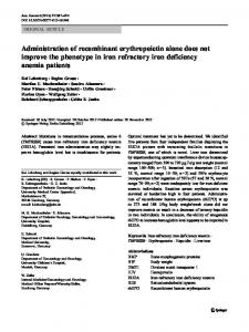
iterations. After 1,500 iterations, the optimal decision variables yielding the optimal feed-rate profile were u0=0.0648 L/h, K=0.0112, and ts=14.75 h (Fig. 2). This optimal feed-rate profile is comparable to the profiles reported earlier [11]; however, the initial feed rates were slightly different. Feed rate profiles achieved by using the modified MCMC and Skolpap et al. [11] were stopped at 35 and 34 hours
Fig. 2. Comparison of optimal feed-rate profiles.
OPTIMIZATION RESULTS Table 5 shows the first five best objective function values obtained from 1,000 and 1,500 iterations. The trends of the objective function values, estimated from two optimal sets of decision variables, were identical. The relative errors of the mean objective function values at 1,500 iterations were in the range of 0.36% to 0.69%. After 1,500 iterations, there was a slight improvement in the objective function values (up to 0.12%) in comparison to those after 1,000
Fig. 3. Comparison of culture volume profiles.
Table 5. Comparison of optimization results at 1,000 and 1,500 iterations Repeat
No. of Elapsed iterations time (sec)
u0 (L/h)
K
ts (h)
J (U/h)
1 2 3 4 5
1,000 1,000 1,000 1,000 1,000
07,980.41 07,667.74 08,197.38 08,495.84 07,507.69
0.0647 0.0688 0.0648 0.0628 0.0701
0.0113 0.0111 0.0101 0.0100 0.0101
14.75 15.75 14.50 13.25 16.00
6,482.2 6,468.7 6,459.1 6,446.9 6,431.9
1 2 3 4 5
1,500 1,500 1,500 1,500 1,500
11,939.20 11,370.55 12,150.91 12,734.53 11,275.45
0.0648 0.0695 0.0649 0.0628 0.0701
0.0112 0.0101 0.0101 0.0100 0.0101
14.75 15.75 14.50 13.25 16.00
6,483.8 6,476.6 6,460.7 6,446.9 6,432.3
July, 2008
Fig. 4. Comparison of α-amylase productivities under optimal feedrate profiles
Fed-batch optimization of recombinant α-amylase production by Bacillus subtilis using a modified MCMC technique
651
Table 6. Comparison of maximum α-amylase productivities obtained from experiment, previous work [11], and a modified MCMC Search technique Experimental result Skolpap et al., 2004 (Reported) A modified MCMC
Optimal value U0 (L/h)
K
ts (h)
J (U/h)
Time peaked (h)
0.0611 0.0619 0.0648
0.0200 0.0112
16.45 14.00 14.75
5474.0 6262.0 6483.4
27.00 34.00 34.75
Fig. 5. Comparison of α-amylase syntheses under optimal feed-rate profiles
Fig. 6. Comparison of protease syntheses under optimal feed-rate profiles
of fermentation, respectively, since the corresponding culture volumes reached maximum values in Eq. (6) (Fig. 3). Fig. 4 compares α-amylase productivities obtained from experimental results and simulation results in previous work [11] as well as from the proposed sampling procedure. The predicted set of decision variables and the corresponding maximum α-amylase productivities achieved from experimental results, previous work [11], and the modified MCMC are illustrated in Table 6. The optimal feed rate trajectory obtained by using the modified MCMC achieved the maximum α-amylase productivities, the objective function, at 34.75 hour of fermentation. As shown in Table 6 and Fig. 4, the maximum α-amylase productivity obtained experimentally, the optimal results reported in Skolpap et al. [11], achieved with a modified MCMC were 5,474 U/h at 27 h, 6,262 U/h at 34 h, and 6,483.4 U/h at 34.75 h, respectively. Apparently, the maximum α-amylase productivities attained by using the modified MCMC was improved 14.4 and 18.4% with respect to the previous work and the experimental result, respectively. The optimal feed rate profiles cannot be verified experimentally due to the limitations of pump speed adjustments. The smallest pump speed increment corresponded to a feed rate change of 0.00238 L/h, while feed rate modification predicted by the modified MCMC was 0.001125 L/h. It should be noted that the experimental observations described above were obtained as a preliminary experiment which served as a basis for fed-batch model development. The proposed modified MCMC enhanced the efficiency of seeking optimal solution over a conventional MCMC procedure. Evidently, further experimentation is needed to confirm the results. Similarly, in Fig. 5 α-amylase activity obtained from experimental results and simulation results in the previous work [11] is com-
Fig. 7. Comparison of biomass productions under optimal feed-rate profiles
pared with activity projected by the proposed sampling procedure. It was found that the proposed sampling procedure improves αamylase activities by 35.9% and 42%, compared with those from experimental and simulation results. As shown in Fig. 6, the maximum protease activity forecast [11] obtained in this work was about 10% higher than that of experimental result. It was shown in Fig. 7 that the biomass production results along the optimal trajectories were comparable. STATISTICAL ANALYSIS The accuracy and acceptability of the simulated results obtained Korean J. Chem. Eng.(Vol. 25, No. 4)
652
W. Skolpap et al.
Table 7. Statistical analysis of objective function values at 1,500 iterations (evaluated at 95% confidence interval) ts (h)
Mean (U/h)
Std. Dev. (U/h)
Upper Bound (U/h)
Lower Bound (U/h)
Relative error (%)
14.75 15.75 14.50 13.25 16.00
6,289.3 6,283.5 6,259.8 6,256.0 6,239.5
0.1851 0.1384 0.2054 0.2672 0.1386
6300.7 6292.1 6272.5 6272.5 6248.1
6277.8 6274.9 6247.1 6239.4 6230.9
0.48 0.36 0.53 0.69 0.36
from the proposed parameter sampling procedure and the Metropolis-Hasting algorithm were statistically examined after neglecting one-third iterations. Given 1,500 iterations, the 500 lowest objective function values were neglected and the remaining 1,000 iterations were use to estimate the relative errors of the objective function values. In Table 7, the 95% confidence interval of the objective function is shown. The calculated mean values of the objective function are all within the interval, which indicates that the optimization based on 1,500 iterations was stationary and sufficiently accurate.
: time lag coefficient : medium flow rate in fed-batch fermentations : bioreactor volume : ammonium nitrogen concentration : protease activity
k20 u V y2 y6
Skolpap et al. [11] reported that ammonium nitrogen was a limiting substrate for the dual-enzyme system and proteolysis caused cell lysis. Ammonium nitrogen concentration (y2 ):
CONCLUSION The proposed modified MCMC parameter sampling procedure using multiple triangular distributions was successfully implemented in searching for a set of decision variables for optimal feed-rate profile determination of a dual-enzyme fed-batch problem. In our experience the optimal decision variables often lie in a region near the edge of the prior distributions that are rarely sampled by the Monte Carlo method. The principal advantages of the proposed method over the existing method are (a) the ability to identify proper parameter values that are located near the tail end or even outside of the parameter sampling ranges by redefining multiple parameter distributions during the sampling procedure, and (b) the ability to reduce random walk behavior by strategically dividing the sampling procedure into learning and searching periods. Given these two advantages, the optimum solution could be achieved and solution convergence could be assured. Moreover, the computational time was minimized by applying multiple distributions and relating the number of iterations with the relative error tolerance of the optimized variable. APPENDIX A
dy NBioAWN⎞ ⎛ dy1⎞ ⎛ NAmyAWN⎞ ⎛ dy3⎞ -------2 = − ⎛ -------------------- ---------------------------- ------⎝ MWBio ⎠ ⎝ dt ⎠ − ⎝ MWAmy ⎠ ⎝ dt ⎠ dt NProAWN⎞ ⎛ dy5⎞ u(y2, 0 − y2 ) - ------- − corX + -----------------------− ⎛ --------------------⎝ MWPro ⎠ ⎝ dt ⎠ V
where corX : correction term for inorganic nitrogen (ammonia) loss due to gas phase stripping MWAmy : formula weight of α-amylase MWBio : formula weight of biomass AWN : atomic weight of nitrogen MWPro : formula weight of protease NAmy : mole fraction of nitrogen in α-amylase NBio : mole fraction of nitrogen in biomass NPro : mole fraction of nitrogen in protease y2, 0 : ammonium nitrogen concentration in feed medium : α-amylase concentration y3 : protease concentration y5 The well-known Luedeking-Piret equation [13] could be used to model the rate of α-amylase synthesis. The model comprises growth associated and non-growth associated terms as follows:
The fed-batch model of α-amylase and protease-producing recombinant B. subtilis ATCC 6015a [11] is listed below. Note that the last term on the right-hand side of the differential equations is a correction for medium inflow or feed rate (u) which affects updated culture volume (V).
α-Amylase concentration (y3):
Biomass concentration (y1):
k5 k6
k1 y 2 u⋅y dy1 ------- = ( 1− e−k t)⎛ -----------------⎞ y1− k3y1 y6 − ----------1 ⎝ k2 + y2 ⎠ dt V 20
where k1 k2 k3
: maximum specific growth rate [µm] : ammonia saturation constant : specific rate of biomass lysis
July, 2008
(A.1)
(A.2)
dy dy -------3 = k5 -------1 + factorAmy( k6y1 ) dt dt
(A.3)
where : growth associated α-amylase productivity constant : non-growth associated α-amylase productivity constant ZAmy y3 − y3, 0 -; ZAmy = ---------------Note that factorAmy =1− -------k18 y1− y1, 0
factorAmy is the ratio of non-growth associated α-amylase synthesis to maximum α-amylase yield. where
Fed-batch optimization of recombinant α-amylase production by Bacillus subtilis using a modified MCMC technique
factorAmy : a feedback modulation term for non-growth associated αamylase formation k18 : maximum α-amylase yield y1, 0 : biomass concentration at initial time of batch period y3, 0 : α-amylase concentration at initial time of batch period Due to the proteolytic effect only on α-amylase activity, the conversion from α-amylase concentration to activity is necessary for the simulation.
α-Amylase activity (y4): dy4 dy u⋅y ------- = k7⎛ -------3 − k8y6⎞ − ----------4 ⎝ dt ⎠ V dt
(A.4)
: conversion factor from α-amylase concentration to activity : rate constant for α-amylase lysis by protease
The model for the biosynthesis of protease enzyme is constructed in a similar vein: Protease concentration (y5): dy5 dy ------- = k17⎛ k9 -------1 + factorPro(k10y1 )⎞ ⎝ dt ⎠ dt
(A.5)
where k9 k10 k17
: growth associated protease productivity constant : non-growth associated protease productivity constant : rate control for protease production
ZPro y5 − y5, 0 - ; ZPro = ---------------Note that factorPro =1− ------k19 y1− y1, 0
: non-growth associated rate constant for ethanol
k21
Lactate concentration (y8): dy8 dy u ⋅ y ------- = k13 y1− k14 -------1 − ----------8 V dt dt
k13 k14
: non-growth associated constant for lactate : growth associated constant for lactate
Acetate concentration (y9): dy9 dy u ⋅ y ------- = k15 y1− k16 -------1 − ----------9 dt dt V
factorPro : a feedback modulation term for non-growth associated protease formation k19 : maximum protease yield y5, 0 : protease concentration at initial time of batch period
where k15 k16
: non-growth associated constant for acetate : growth associated constant for acetate
During the early stages of the fermentation, citrate served as a supplementary carbon source and was consumed as shown in the following rate expression: Citrate concentration (y10): dy 1⎞ − 0.5 ⋅ ⎛ -------1 + dy ⎝ dt ------dt ⎠ dy10 --------- = -----------------------------------------YX/Cit dt
YX/Cit : a yield of biomass per gram of citrate [g biomass/g citrate]
Starch concentration (y11): dy11 MWSt ⎧ 1 AWC dy1 AWC dy3 AWC dy5 --------- = ------------- ⋅ ⎨− ---- ⋅ ------------- ⋅ ------- − ----------------- ⋅ ------- − ---------------- ⋅ ------dt AWC ⎩ k4 MWSt dt MWAmy dt MWPro dt AWC dy8 AWC dy9 AWC dy - ⋅ ------- − ----------------- ⋅ ------- − NCit -------------- ⋅ YCit/St ⋅ --------10− --------------MWLac dt MWHAc dt MWCit dt AWC dy7 ⎫ u(y11, 0 − y11) - ⋅ ------- + ---------------------------− -----------------MWEtOH dt ⎬⎭ V
Protease activity (y6): (A.6)
where : conversion of protease concentration to activity : non-growth associated protease productivity constant during ammonium nitrogen limitation
The formation of ethanol, lactate, and acetate strongly depended on the C : N ratio and the availability of oxygen as expressed below: Ethanol concentration (y7): dy7 u⋅y ------- = − k21 y1+ 0.028 − ----------7 dt V
where
(A.10)
where
Similarly, model structure for protease activity mimics the model for α-amylase activity:
k11 k12
(A.9)
The stoichiometric coefficients for Eq. (11) were derived by metabolic flux analysis. The carbon balance is converted to starch equivalents in the following manner:
where
dy u⋅y dy -------6 = k11 ⎛ -------5 − k12 y6⎞ − ----------6 ⎝ dt ⎠ V dt
(A.8)
where
where k7 k8
653
(A.7)
(A.11)
where k4 : biomass yield constant (YX/S) AWC : atomic weight of carbon MWCit : molecular weight of citrate MWEtOH : formula weight of ethanol MWHAc : formula weight of acetate MWLac : formula weight of lactate MWSt : formula weight of starch NCit : number of carbon atoms in one mole of citrate y11, 0 : starch concentration in the fed-batch feed medium YCit/St : mass equivalent of citrate [g citrate/g starch] An amino acid supplement of isoleucine (Ile) and threonine (Thr) is beneficial for biomass as well as α-amylase production as indicated by metabolic flux analysis [15]. Korean J. Chem. Eng.(Vol. 25, No. 4)
654
W. Skolpap et al.
Isoleucine concentration (y12): ⎧ dy dy12 1 ⎞⎞ --------- = corIle⎨⎛AABio ⋅ IleBio ⋅ 0.5 ⋅ ⎛ -------1 + dy ⎝ ⎝ dt ------⎠⎠ dt dt ⎩ ⎫ dy 3 ⎞⎞ + ⎛ IleAmy ⋅ 0.5 ⋅ ⎛ -------3 + dy ⎬ ⎝ ⎝ dt ------⎠ ⎠ dt ⎭ u(y12, 0 − y12) dy 5 ⎞ ⎞ + --------------------------+ ⎛ IleAmy ⋅ 0.5 ⋅ ⎛ -------5 + dy ⎝ ⎝ dt ------V dt ⎠⎠
(A.12)
where AABio : mass fraction of protein in biomass corIle : correction term for y12 IleAmy : mass fraction of isoleucine in α-amylase IleBio : mass fraction of isoleucine in biomass protein IlePro : mass fraction of isoleucine in protease y12, 0 : isoleucine concentration in feed medium
(A.13)
where corThr : correction term for y13 ThrAmy : mass fraction of threonine in α-amylase ThrBio : mass fraction of threonine in biomass protein ThrPro : mass fraction of threonine in protease y13, 0 : threonine concentration in feed medium As in case of Ile, the external source of Thr accounts for 15% of the total Thr requirement. Evidently, the external supply of both Ile and Thr was adequate to achieve the enhancement of α-amylase synthesis. The differential equation for the volume change as the function of the feed rate is straightforward as expressed in Eq. (1). APPENDIX B ESTIMATED VALUES OF MODEL PARAMETERS [3]
k10 k20 k 30 k 40 k 50 k 60
0.376 0.253 1.707×10⁻⁴ 0.721 1.543×10⁻⁶ 1.512×10⁻²
July, 2008
Model parameter k 14 k 15 k 16 k 17 k18 k19
0.399 5.3×10⁻³ 0.880 0.890 0.920 0.000 NE
NE denotes an unevaluated parameter value due to citrate depletion prior to fed-batch fermentation.
NOMENCLATURE
⎧ dy13 dy 1 ⎞⎞ --------- = corThr⎨⎛ AABio ⋅ ThrBio ⋅ 0.5 ⋅ ⎛ -------1 + dy ⎝ ⎝ dt ------dt dt ⎠ ⎠ ⎩
Fed-batch value
k 20 k 21 corAmy corBio corPro corX YX/Cit
This research has been financially supported by the Thailand Research Fund under grant number MRG4780214.
Threonine concentration (y13):
Model parameter
10.177 1.208×10⁻³ 2.689×10⁻³ 0.183 10.273 1.068×10⁻² 1.191×10⁻⁴
ACKNOWLEDGMENT
The value of this correction factor was obtained by metabolic flux analysis. Presumably, the bacterium had no absolute external requirement for Ile and was capable to synthesize most (80%) of the Ile internally. The differential equation for Thr is:
⎫ dy + ⎛⎝ ThrAmy ⋅ 0.5 ⋅ ⎛⎝ -------3 + dy -------3 ⎞⎠ ⎞⎠ ⎬ dt dt ⎭ u(y13, 0 − y13 ) dy 5 ⎞ ⎞ + --------------------------+ ⎛ ThrAmy ⋅ 0.5 ⋅ ⎛ -------5 + dy ⎝ ⎝ dt ------V dt ⎠ ⎠
k 70 k 80 k 90 k 10 k 11 k 12 k 13
Fed-batch value 5.626×10⁻⁷ 2.481×10⁻³ 9.970×10⁻⁷ 0.152 0.472 5.684×10⁻²
AABio : mass fraction of protein in biomass {0.55} AWC : atomic weight of carbon {12.01} AWN : atomic weight of nitrogen {14.01} corAmy : correction term for ammonium nitrogen consumption of αamylase corBio : correction term for ammonium nitrogen consumption by biomass formation corIle : correction term for y12 {0.2} corPro : correction term for nitrogen consumption of protease corThr : correction term for y13 corX : correction term for inorganic nitrogen (ammonia) loss due to gas phase stripping df : degree of freedom E : expected parameter value Eq : expectation in the qth row of the same column factorAmy : a feed back modulation term for non-growth associated α-amylase formation factorPro : a feed back modulation term for non-growth associated protease formation IleAmy : mass fraction of isoleucine in α-amylase {0.053} IleBio : mass fraction of isoleucine in biomass protein {0.05999} IlePro : mass fraction of isoleucine in protease {0.050} J : objective function value [U/h] Jmax : maximum theoretical productivity value [U/h] : maximum specific growth rate [h−1] k1 : ammonia saturation constant [g/L] k2 : specific rate of biomass lysis [L/g·h] k3 : biomass yield constant (YX/S) [g cell/g starch] k4 : growth associated α-amylase productivity constant [g Amy/ k5 g cell] : non-growth associated α-amylase productivity constant [h−1] k6 : conversion factor from α-amylase concentration to activity k7 [×10−3 U/g] : rate constant for α-amylase lysis by protease [×103 g/U(h)] k8 : growth associated protease productivity constant [g Pro/ k9 g cell] k10 : non-growth associated protease productivity constant [h−1] k11 : conversion of protease concentration to activity [×10−3 U/g] k12 : non-growth associated protease productivity constant dur-
Fed-batch optimization of recombinant α-amylase production by Bacillus subtilis using a modified MCMC technique
ing ammonium nitrogen limitation [×103 g/U(h)] k13 : non-growth associated constant for lactate [h−1] k14 : growth associated constant for lactate [g Lac/g cell] k15 : non-growth associated constant for acetate [h−1] k16 : growth associated constant for acetate [g HAC/g cell] k17 : rate control constant for protease production k18 : maximum α-amylase yield [g Amy/g cell] k19 : maximum protease yield [g Pro/g cell] k20 : time lag coefficient k21 : non-growth associated rate constant for ethanol [h−1] K : exponential constant term in feed rate equation MWAmy : formula weight of α-amylase {25.18} MWBio : formula weight of biomass {26.08} MWCit : molecular weight of citrate {193} MWEtOH : formula weight of ethanol {23.04} MWHAc : formula weight of acetate {30.03} MWLac : formula weight of lactate {30.03} MWPro : formula weight of protease {26.94} MWSt : formula weight of starch {26.96} NAmy : mole fraction of nitrogen in α-amylase {0.274} NBio : mole fraction of nitrogen in biomass {0.224} NCit : number of carbon atoms in one mole of citrate {6} NPro : mole fraction of nitrogen in protease {0.268} Oq : observation in the qth row of the same column P : desirable product (α-amylase) concentration [g/L] q : proposal distribution of the parameter Q : a number of data points in any column r1, r2 : random numbers in the range of [−1, 1] : variance s2 t : fermentation time [h] : time at observation taken [h] tk : switching time or starting time for feeding [h] ts T : total time period [h] ThrAmy: mass fraction of threonine in α-amylase {0.0712} ThrBio : mass fraction of threonine in biomass protein {0.04523} ThrPro : mass fraction of threonine in protease {0.06468} u : medium flow rate in fed-batch fermentations [L/h] V : bioreactor volume [L] : biomass concentration [g/L] y1 : ammonium nitrogen concentration [g/L] y2 : α-amylase concentration [g/L] y3 : α-amylase activity [U/mL] y4 : protease concentration [g/L] y5 : protease activity [U/mL] y6 : ethanol concentration [g/L] y7 : lactate concentration [g/L] y8 : acetate concentration [g/L] y9 y10 : citrate concentration [g/L] y11 : starch concentration [g/L] y12 : isoleucine concentration [g/L] y13 : threonine concentration [g/L] YCit/St : mass equivalent of citrate [g citrate/g starch] {0.48} YX/Cit : yield of biomass per gram of citrate [g cell/g citrate] YX/S : theoretical cell yield based on substrate consumed [g cell/
655
g substrate] Greek Letters : the probability of acceptance of a sampled value : a probability of a χ2 statistic : the mean parameter : the parameter value : stationary distribution of the parameter
α χ2 δ θ π
Subscripts i : the ith parameter q : the qth data point of any state variable Superscripts better: better parameter value best : the best parameter value j : the jth iteration min : minimum value max : maximum value REFERENCES 1. J. M. Nougués, M. D. Grau and L. Puigjaner, Chemical Engineering and Processing, 41, 303 (2002). 2. L. Z. Chen and S. K. Nguang, ISA Transactions, 41, 409 (2002). 3. D. Sarkar and J. M. Modak, Chem. Eng. Science, 58, 2283 (2003). 4. L. Z. Chen, S. K. Nguang, X. D. Chen and X. M. Li, Biochem. Eng. J., 22, 51 (2004). 5. V. K. Jayaraman, B. D. Kulkarni, K. Gupta, J. Rajesh and H. S. Kusumaker, Biotechnol. Prog., 17, 81 (2001). 6. A. Patkar, D. H. Lee and J. H. Seo, Korean J. Chem. Eng., 10, 146 (1993). 7. J. E. Cuthrell and L. T. Biegler, Comput. Chem. Eng., 13, 49 (1989). 8. H. C. Lim, Y. J. Tayeb, J. M. Modak and P. Bonte, Biotechnol. Bioeng., 28, 1408 (1986). 9. W. Mekarapiruk and R. Luus, Can. J. Chem. Eng., 79, 777 (2001). 10. W. Mekarapiruk and R. Luus, Ind. Eng. Chem. Res., 39, 84 (2000). 11. W. Skolpap, J. M. Scharer, P. L. Douglas and M. Moo-Young, Biotechnol. Bioeng., 86, 706 (2004). 12. W. Skolpap, J. M. Scharer, P. L. Douglas and M. Moo-Young, Songklanakarin J. Sci. Technol., 27, 1057 (2005). 13. R. Luedeking and E. L. Piret, J. Biochem. Microbiol. Technol. Eng., 1, 431 (1959). 14. A. Constantinides and N. Mostoufi, Numerical methods for chemical engineers with MATLAB applications, Prentice-Hall Inc., New Jersey, 323-340 (1999). 15. W. Skolpap, Bioprocess optimization using metabolic engineering approach, Ph.D. Thesis, University of Waterloo, Waterloo, Ontario (2003). 16. D. C. Montgomery, G. C. Runger and N. F. Hubele, Engineering statistics, 4th Edition, John Wiley & Sons, New York (2006). 17. C.-K. Min, Comput. Stat. Data An., 27, 171 (1998). 18. W. R. Gilks, S. Richardson and D. J. Spiegelhalter, Markov chain Monte Carlo in practice, Chapman & Hall, London, UK (1998).
Korean J. Chem. Eng.(Vol. 25, No. 4)