are considered: joiniangle a'[!d velocity.feedback with (GRC) and without (IJe) cross ... The tech- niques used to analyze these distributed flexible systems are of.
W. J. BOOK Assistant Professor of Mechanical Engineering, Georgia Institute of Technology, Atlanta, Ga.
O. MAIIIA·NElO Assistant Professor of Mechanical Engineering, Escola Politecnia da U.S.P., Sao Paulo, S. P., Brazil
D. E. WHITNEY Section Chief, Charles Stark Draper Lab., Cambridge, Mass.
Feedback Control of Two Beam, Two Joint Systems With .Distributed· Flexibility! The control. of the flexible motion in a plane of two pinned beams is addressed with application to remote manipulators. Three types of linear feedback control schemes are considered: joiniangle a'[!d velocity.feedback with (GRC) and without (IJe) cross joint feedback, and· feedback of flexi,lJlestate variables (FFC). Two models of the distributed flexibility are presented ,alO1igivith some results obtained from them. The relative merit of the three control schemes ,is discussed.
I ntrod uction Manipulators are found in industrial and research environments which.are too hazardous or unpleasant for a human worker. Requirements for safety and improved working conditions are becoming more stringent due to legislation and collective bargaining, while international competition requires that ever higher productivity be achieved. Computer commanded industrial manipulators can potentially meet the increased demands of both worker safety and productivity, but improved manipulator arm designs and controls are needed. A study of various alternative joint torque control schemes for the planar motion of two pinned flexible beams has been conducted. This type of system is displayed schematically in Fig. 1. The immediate application for the results is in the area of manipulator arms and this application flavors the analysis. The specific results are of interest outside this area since many beamlike components are found in mechanical hardware. The techniques used to analyze these distributed flexible systems are of even more general interest. ManipUlator arms require a reasonable accuracy in response
'This work was supported by NASA Marshall Space Flight Center under contract NAS8-28055 to the Department of Mechanical Engineering, Massachusetts Institute of Technology, and by Fundacao de,Amparo a Pesquisa do Estado de Sao Paulo, Brazil. Contributed by the Automatic Control Division for presentation at the Winter Annual Meeting, Houston, Texas, November 3D-December 5, 1975, of THE AMERICAN SOCIETY OF l\1ECHANICAL ENGINEERS. Manuscript received at ASME Headquarters, July 23, 1975. Paper No. 75-WA/Aut-26. Copies will be available until August, 1976.
of the arm's end point to input commands to the joint contro system. This accuracy is deteriorated by structural deformation especially when the deformation is oscillatory. The simplest way to eliminate these vibrations is to increase the rigidity of the arm, which ultimately means increasing the load bearing material. Adverse effects of this practice have been increased torque and power requirements, higher feedback gains, higher total system weight, and a typical payload capacity of 10 percent of the arm weight [16].2 Thus in the interest of better arm design one would like to understand the limitations imposed by the structure on arm performance. These limitations are intimately related to the type of control scheme used and can be overcome to some extent by recognizing the flexible nature of the arm structure when establishing the control scheme and its param7 eters.
Characterization of the Problem This study was conducted to yield practical design information and yet recognize the essential distributed nature of the manipulator structure. Prior results [5, 6, 9, 14, Hi] in optimal control of distributed systems are largely for systems defined by a single set of partial differential equations, instead of two interacting sets as is the case here. The systems studied here include distributed beams considered to be adequately modeled by the Bernoulli-Euler beam equations. Control torque is applied at hinged joint~ between the beams and between the inboard or proximal beam and an inertial ground. Lumped masses at the distal end of each beam representing 'Numbers in brackets designate References at end of paper.
1 Discussion on this paper will be accepted at ASME Headquarters until .January 5, 1976
control
~I
rigid ma .. 8 7
control Q.4 angle A 5 Fig.! Schematic system and nomenclature
actuator and payload mass are considered. A feedback control law is desired which commands torque on the basis of feedback which could be measured at or observed from measurements at discrete points. The control system serves the purpose of tracking desired trajectories as well as regulating the system position in the face of disturbance loadings. The position of the dominant system poles was the major consideration when judging the relative merit of competing arm systems. Large eigenvalue absolute value with "adequate" damping is indicative of high arm bandwidth which is necessary for manipulators capable of fast accurate small motions. Higher modes were required to remain stable and time responses obtained from both linear and nonlinear models were used to fll1'ther check the system behavior.
System Models Used Two complimentary models were employed in this study. One is basically a time domain model employing truncation of a modal description of the beam shapes and allows nonlinear effects to be included in the system simulation. The other is a frequency domain technique which requires linear assumptions including small motions about an equilibrium position with no Coriolis, centrifugal or gravity forces, but it can easily describe various beam configurations and includes distributed effects with no modal truncation. The two models agree very well in those situations where comparable results could be obtained and accurately predict experimenta1 results obtained. A.
Frequency Domain Model. The frequency domain model of
the arm was implemented via the transfer matrix methods which have found frequent use in applied mechanics but only rarely for purposes of control. With the use of numerical techniques the frequency domain model becomes a versatile design tool. Transfer Matrix Formulation. The transfer matrix (t.m.) state variables3 chosen for description of the arm are those used by Pestel and Leckie [11] for representing the flexural vibrations of a beam, and are displayed in Fig. 2. Because slender beams are vastly more rigid in compression than in flexure, four t.m. state variables adequately describe the general planar motion of an arm system. A transfer matrix for various arm model elements such as controlled joints, joint angles, Bernoulli-Euler beams, and rigid inertias can be constructed. These matrices relate the Laplace transform of the t.m. state variables at one of the two stations of the elements to the Laplace transform of the t.m. state variables at the other station. The product of several transfer matrices constitutes a complete description of those elemcnts clamped consecutively together since the t.m. state
'The term transfer matrix variables (..bbreviated "t.m. state variables") is used to avoid cOllfusion with state variables involved ill a state variable formulation of modern control theory.
2
-W] [- dilPlacement] "'.. angle moment [M V
Ihear force
Fig.2 Transfer matrix representation and state variables
variables are identical at the common station of two elements. Fig. 2 displays a possible arm and its transfer matrix implementation. By imposing boundary conditions at either end of the arm model one specifies some of the t.m. state variables related by the product matrix. The controlled ioint transfer matrix relates the t.m. state vectors at stations i and i + 1 as follows:
o l/k(s) Xi
=
1
o where k(s)
s k(s)
=
M'+1
!fi - !fi+l
the Laplace variable the transfer function which relates the joint angle to the control torque applied.
The only work which will be presented here using the transfer matrix model is for k of the form k(s) = k p
+ sku
(2)
That is, control torque equal to the sum of the joint angle and its derivative, each times appropriate gains. Numerical Techniques in Implementation. The transfer matrices of some elements, especially distributed beams, are reasonably complex and are best evaluated by digital computer. The matrix product is then taken numerically and numerical techniques are necessary to extract useful information from the model. The first step in obtaining useful information from the matrix relation of the model equation (3).
zo
=
U(s)Z,.
(3)
is to constrain certain of the t.m. state variables and thus provide system boundary conditions. If the four constrained t.m. state variables are all zero one can find in equation (3) two homogeneous equatiqns linear in two t.m. state variables [It station n. The determinant' of the coefficients (which are a function of the complex vadf1lJ~e.s)
Transactions of the ASME
If now U1E
= flexible displacement at end of beam 1
11
length of beam I
ls
length of beam 2
+ [0 Fig.3
Coordinate systems in the time domain model
must equal zero for a nontrivial solution. The values of 8 at which this condition is satisfied are the eigenvalues of the system. The present work utilized two dimensional numerical searches over the complex plane to find the eigenvalues from this relation. If one or more of the constrained t.m. state variables are pure sinusoids of constant amplitude and a single frequency w the steady-state forced frequency response can be found. Equation (3) is evaluated with 8 = jw and with the constrained t.m. state variables equal to the complex amplitude of the sinusoidal forcing function. From these samples of the frequency response the time response can be calculated via the fast Fourier transform algorithm of Cooley and Tukey [1]. Details of this implementation are found in [2]. B. Time Domain Model. The derivation of the time domain model is based on the description of the system in Fig. 3. In order to describe the motions, three reference frames and their unit vectors [4] can be defined:
[OXY] an inertial reference frame with origin at joint 1 and unit
vector {U} [O,lhY1] a reference frame with origin at 0, axis Xl tangent to beam
- 1 at point 0 and unit vector
{ud
where cO
Also, the two angles can be defined: Ol(t) is the angle between the axes Xl and X 02(t) is the angle between the axes Xl and X2 If now a new system is defined as being formed by two segments 001 and olb a having the angle O2 at 01, the overall motion can be 1JI\derstood as a motion of a hypothetical rigid system [0 01 Oa] !1I\d a flexible motion of the beams 1 and 2 with respect to this . moving system. Kinematic Description. As indicated in Fig. 3, any point Pi can be specified if a new variable U,(Xi, t) is defined as being the coordinate of the flexible motion with respect to the reference frame [Ox,y,]. The vector position of point Pi would be:
+ y,uu'
=
{ud t { y,Xi}
{ud t {::
(5)
sin O.
V = m1g11(1 - c01)/2
+ mj(71l(t~,?01)"+ m2(J,
}(l - C(Ol + O
+
+ 1 (1 2
- C(Ol
+ 02))]
2 ))
]
-
~
[h(l - COl)
/~ + mpg[ll(l -
J:
11
E1Il (
COl)
:::~ Ydx (7)
where g is the component of gravity acceleration in the OX direction. Ed1, and Ed2 are the stiffnesses of links 1 and 2, respectively, assumed constant for the purpose of this model. In order to write the equations of motion of the system the method of assumed modes [8] is used. A solutioll of the flexible motions is assumed to be a linear combination of admissible functions c±>,j (x,) (which satisfies the essential boundary conditions [3] for the reference frame used) multiplied by time dependent generalized coordinates qij(t). Thus the flexible motion is written as n
Ul = ~ c±>li(Xl)qli(t)
}
=
{U}t[Ol]t {:: }
Assuming small deflections one can consider the paths of points 01 and Op as straight lines normal to the respective reference frames. Then, as shown in Fig. 3, the vector position of any point P 2 on beam 2 will be Rd2 = 001
02 } ]
U
The potential energy of the system is assumed to be composed of the energy associated with the rigid motion plus the elastic potential energy of the beams. Assuming OX as the reference position, the total potential of the system for small Ul and U2 can be approximated by
The vector position of any point in beam 1 is
Ral =
=
{
These position. vectors. can be differentiated with respect to time to obtain Rd1 and R d2 , the velocity vectors. For any mass mj concentrated at joint 2 the position Rj and velocity Rj will be the same as for the end of beam 1 and for any payload of mass ml' and moment of inertia about its center of gravity J p the position Rp and velocity will be the same as for the end of beam 2. This result can be used to write the total system kinetic energy:
tangent to beam 2 at point O2, and unit vector {U2}. The unit vectors can be related by rotation matrices 01 and O2 as follows:
XiU.,
cos 0 and 80
.
[02X2Y2] a reference frame with origin at joint 2, with axis X2
Rai=
=
2]'
+ 0 0 + 02P2 1 2
''''1
(8)
n
U2 = ~ c±>2i(X2)q2,(t) i=1
Assuming that the amplitude of the higher modes of the flexible links are very small compared with the first ones, the system
Journal of Dynamic Systems, Measurement,and Control
3
can be truncated with 11 equal 2, resulting in a six degree-offreedom problem. If the 1.0 the system is no longer adequately described by the complex pair alone. The maximum value of the dominant eigenvalue at which adequate damping can be achieved depends on the relative stiffness and mass of beams 1 and 2, the payload mass, and on the angle of joint 2. The critical value seems in a wide variety of cases to be approximately one-half of w" the natural frequency of the arm with both joints clamped. For two joints controlled with IJC the rigid design procedure is less straightforward and arbitrary pole placement cannot be achieved. An acceptable relative pole pattern is obtained for
Cross section area moment of inerti!l:
kl
T14(1 - k.4)/4
50 k2J1.1/ jJ.2
clIO k2J1.1/ (p J1.2) Tl
outer radius of beam 1
k,
geometric factor which, for a concentric circular cross section, corresponds to (inner radius) /(outer radius).
C2
The parameters in Table 1 can be combined to yield any product of the basic dimensions, F, L, and 111 for nondimensionalizing the parameters of the system. In addition the dimension 7' can be obtained as
The non dimensional value of a parameter will be designated with a bar, for example for a frequency W = - js
W=
W/Wd
For all the results displayed here!
II = l2, i.e. II = 12 == 0.5 The nondiinensional stiffness of beam 2, El2 = Eld Ell iH one o.f the important design parameters which, with the nondimen!'iIOnal payload mass iIi,p, affects the arm ban~hvidth 9\}tain!1bl e. For 'inp ;= 0 the ,5election of El2 lel-is than one ,appreciably raises the bandwidt,h obtainp,ble, while for 'ilL" = 1 thj~ qges not seem
1.17 k!/p
where kl, k2 are angular position feedback gains of joints 1 and 2 respectively and CI, C2 are angular velocity feedback gains of joints 1 and 2, respectively. P -
-
~
k2 J1.123/3
+ rnpl22
Fig. [) displays for equal beams, no payload and, Cl!2 = 0 the two most dominant eigenvalues as the parameter p is increased, increasing system bandwidth. Once again wc /2 is an approximate limit for the bandwidth of this flexible system and for other systems of this type using IJC. IJe is inherently stable in all cases, since the system could be realir.ed with strictly passive components. Impulse responses obtained from inverse transforming the frequency response show '{ery little effect of the higher system modes. More detailed consideration of this control scheme is found in [2]. GRC Root Loci. The simple IJC control has been characterized as \i,nited to approximately wc /2 by system flexibility. The more complicated forms of control should demonstrate some improvemi!nt to justify their increased complexity. G RC gains for Fig. 6 were determined from equntion (11) for WI = W2 and Sl = S2. It was found for WI ¢ W2 that the deLeriorn,tion of damping on
Journal of Dynamic Systems, Measurement, and Control
5
I
-,--~--~-
6
2.0
p=l.§
0!04
61.6
~N
?' 104 6
1:2
1.0
0.03
!
"
0.02
.. 0
C\I
,.... >C
I~
60.8
~.o~
,.,...
.5.
60.6
4g.4
co
!!l
o
v ci
~
P,
6p;;Q.2
g;
~rr,
0.5
0.0
1.0
-2.0
a.s
a.D
~.S
~-~I.O
Time
".0
4.0
3.5
r
Fig.7(a) Angle response to torque impulse at joint Z for GRC. EI, 0,1667, = 0, mp = 0
a,
Re(jw>x2/II+EI 2 Fig. 5 Dominant eigenvalues at IJC attempts higher ban!lwidth. £1, = 1.0, '7 = Q~ iff~ = 0
~D;r,:,,~
f~
the dominant eigenvalue occurred at lower eigenvalue magnitudes and that in some cases the higher modes were unstable. As Fig, 6 indicates in comparison with Fig. 5 an improvement of 100 percent in the maximum arm bandwidth permitteq by the flexible arm structure can be achieved py in~l1-!ding the orosEl joip.t gains. This is of course variable with'payload mass /j:p.d r~l~Hye masses and stiffnesses of the beams, but eigenvalues with magnitude on the order of the clamped natural frequency can be achieved. It should be mentioned that this result is obtained using a rigid design procedure, and gain adjustments based on the sensitivity of the poles may yield improvement. Efforts to date using sensitivities have been discouraging, however. The Simon Mitter algorithm [12, 13] as implemented by Maizza-Neto was used to determine the gains for the matrix F of feedback gains as described in equation (12). The eigenvalues of the flexible model could be moved in an arbitrary manner by the algorithm with practical limitations arising due to the sensitivities of the eigenvalues to perturbations of the system parameters, including feedback gains and joint angles. Due to these practical limitations it is not possible to conclude that this control configuration and design method will result in superior performance, especially in application to manipulator arms. C.
Results Using FFC and the Simon Mitter Algorithm.
cO
~
. ! ~
~o
S 0
-5 -~o
I
-'5.S!=:-'.3 0.0
1..'5
~.O
0.5
2_0
lir.le
a.s
T
Fig.7(b) Angle resp0!1,se to torqJ,e impulse at joint Z for FFC. EJ, = 0.1667, = 0, mp = O. -
a,
Fig, 7(a) and (b) compares GRC to. FFC based on time responses from torque impulses 'at joint 2. The eigenvalues requested from the Simon Mitter algorithm were identical but the responses of Fig. 7 are markedly different. This results from different methods of resloving the nonuniqueness of the gains. The gains are completely different as are the eigenvectors. The lower torque requirements observed for GRC in Fig. 8 favor that,
--r_____---,9.0 I
,--_ _ _ _ _ _----._ _ _-q--_ _ _ Path (\f first two eigenvalues as r;: r;, '" r;2varies.
\ \ ~\
B.O
6\
---lines of constant r; for first two eigenvalues.
\ \
a. -12.0 -11.0 -10.0
-9.0
-8.0
-7.0 -6.0 -5.0 Re(2J;;!(~))
-4.0
Fig. 6 Dominant eigenvalues as GRC attempts higher bandwidth. £1, = 1.0, = 0·, ll = 0
a,
6
m
el tJO.~1 torque
-sr-3 L_---'-_ _----L_ _..L_ _L-_---'-_ _--L_ _-L_----l 0.0
0.5
:1..0
1.5
2.0
2.5
9.0
3~S
4.0'
Tiole f
Fig. 8(q) Torque response to torque impulse at joint Z for GRC. £1, = 0.1667, '= 0, mp = O.
a,
Transactions of the ASME
I
0 .. 10 0 .. 09
n,oa
~
3,0
0
'"
0.07
Z,5
0.06 0
~ ~
0.05
.!
z.o
0.04
o Gains from ffip =0 applied to ffip =0
0.03
!
~
x Gains from ffip =I applied to fiip= I
0 .• 02
-0 .. 0:10.0
elbow torque 0.5
tJ ... 0
1. .. 5
2.0
2.5
3.0
£1,
8(b)
'"
Gains from 1fip =I applied to 1Iip =0
1,0
~
.
"I~'"" .§
0,5
ElZ =0,8
Time T
Fjg.
tJ
"" Gains from fiip =0 applied 10 iiIp= I
0.0"1 0.00
1.5
Torque response to torque impulse at joint 2 with FFC.
-3.0
= 0.1667, ", = 0, mp = o.
-Z,5
-Z,O
-1.5
-1.0
-0,5
Re (jw)x Z/( JEiZ+1 )
scheme over FFC. Table 2 indicates another disadvantage of modal control for the application at hand. Listed there are the eigenvalues after joint 2 has moved from the design point of 0° to 90°. Certain of the higher poles show positive real parts indicating instability. GIlC eigenvalues for the same angle change remain stable. In some cases modal control Inay be useful if the system is constant and accurately known, but for manipulator application ' this tends not to be th~ case. D. Arm Operation With Constant GRC Gains. The normal operation of a manipulator arm results in large joint angle and payload changes. These changes in the sYHtem change eigenvalues and arm dynamics. It is desireable to maintain constant gains for system simplicity if the resulting performance is acceptable. Fig. 9 displays the shift in arm eigenvalues when the design payload of mp has been removed. Also displayed are the eigenvalues which .could be obtained if the gains were adjusted to account for the altered system. These results indicate that constant ga,ins, if used, should correspond to the Case where the arm carries a payload. The variation of dominant roots for joint 2 varying from 0 deg to 90 deg are shown in Fig. 10 indicating some deterioration in the damping ratio of one of the two dominant pole pairs.
Fig.9 Dominant eigenvalues for constant GRC gains with changes in payload. £1, = 0.8, "2 = O.
are derived. The models derived were used to explore three control schemes. GRC and IJC were based on the joint angle measurements with and without interjoint feedback, respectively. FFC feeds back the flexible modes of the beam as well. IJC is limited in the bandwidth it can provide to approximately wc/2 by inadequate damping. GRC shows marked improvement with a slight increase in complexity providing bandwidth as high as We. FFC as implemented showed high sensitivities to parameter perturbations and somewhat higher torque requirements, and requires much more complexity, severely detracting from its usefulness for manipulators.
References 1 Bergland, G. D., "A Guided Tour of the Fast-Fourier Transform," IEEE Spectrum, July 1969. 2 Book, Wayne, J., "Modeling Design and Control of Flexible Manipulator Arms," PhD thesis, Dept. of Mechanical Engineering, Massachusetts Institute of Technology, 1974.
Table 2 Eigenvalues of flexible model GRC a2 = 0 REAL IMAG. -1. 4130 ± 1. 4522 -1.3817 ±1.6114 -11.167 0.0000 -5.9610 ±33.406 -5.6658 ±68,974 -55.790 ±103.55 -489.59 0.0000
£/2
FFC a2 = 0 REAL -1.3309 -1.4138 -11.847 -6.0627 -5.8295 -54.836 -482.15
Conclusions Two useful procedures have been presented for mudeling the planar motion of hinged flexible beams with controlled joints. One procedure incorporates transfer matrices and numerical techniques to derive useful information from the frequency domainlllodel. The other procedure incorporates a truncated modal de~cription of dynamic beam flexllJ'e. The flexible ane! "rigid" components of the po~ition are uHed to wril'e Lagrallge'~ equation for the system, and thus the approximate equations of motioll
IMAG. ±1.4407 ±1.6263 0.0000 ±33.458 ±67.830 ±103.54 0.0000
= 0.1667, mp = 0 FFC a2 = 11"/2 (designed for a~ = 0) REAL -0.4136 -2.2831 -30.070 -18.631 0.2469 -42.319 -375.39
IMAG. ±0.9630 ±1.6225 0.0000 ±30.300 ±43. 797 ±96.351 0.0000
3 Crandall, S. H., Engineering Analysis, McGraw-Hill, 1956. 4 Crandall, S. H., Karnopp, D. C., Kirtz, E., and PridmoreBrown, D. C., Dynamics of 111echanical and Electromechanical Systems, McGraw-Hill, 1968. 5 Koehne, Manfred, "Optimal Feedback Control of Flexible Mechanical Systems," Proceedings of IFAC Symposium on the Optimal Control of Distributed Parameter Systems, Banf, Canada, 1971. . 6 Komkov, Vadim, Optimal Control 'Theory fol' the. Dampmg of Vibration of Simple Elastic Systems, Lecture Notes 1Il iVlathematics, No. 253, Springer-Verlag, 1972.
Journal of Dynamic Systems, Measurement, and Control
7
, - - - - - - - - " - - - - - - - - - , . 1.8
\
~~ 90·
\
\
\
\
,, \
1.4
1.2 90"
1.0 I~
]" 0.6
\
, \
damping ratio
1.6
0.0 \
\
\
0.'
\
,o.707-,\ \
, \
,
O.t
f.,,---.,.-r--r---.,.-r---:-r-----:-r--r--.---:" 0.0 -2.8 -2.4 -2.0 -1.6 -1.2 -0.8 -0.4 0.0
-3.2
net;;) Fig. 10_Dominant eigenvalues for constant GRC gains with changes in a,. Eh = O.1667m mp = O.
7 Maizza-N\3to, o ctavi , "Modal AnaJysis and Control of Flexible Mahiptilator Arms," PhD thesis, Dept •. of Mechanical Engineering, Massachusetts Institute of Technology, 1974. 8 Meirovitch, L., Analytical Methods in Vibrations, The MacMillian Co., 1967. 9 Mil'ro/ John, liAutomatic Feedback Control of Ii, Vibrating Flexible Beam," MS thesis, Dept. of Mechanical Engineering, Massachusetts Institute of Technology, Aug. 1972. 10 Nevins, J. L., Whitney, D. E., and Simunovic, S. N., "Report on Advanced Automation, System Architecture for Assembly Machines," Charles Stark Draper Laboratory Report, R 764, Nov. 1973. 11 Pestel, Eduard C." and Leckie, Frederick A., Matrix Methods in Elasto-Mechanics, McGraw-Hill, 1963. 12 Simon, J. D., "Theory and Application of Modal Control," PhD thesis, Case Institute of Technology, 1967. 13 Simon, J. D., and Mittel', S. K., "A Theory of Modal Control," Information q,nd Control, Vol. 13, Oct. 1968, pp. 316353. 14 Van de Vegte, J., Op·timal and Constrained-Optimal Controls for Vibrating Beams," JACC Paper 19-C, 1970, p. 469. 15 Vaughan, D, R., "Application of Distributed Parameter Concepts to Dynamic Analysis and Control of Bending Vibrations," Journal of Basic Engineering, TRA:Ns. ASME, Series D, Vol. 90, No.2, p. 157. 16 Whitney, D. Eo, Book, W. J., Lynch, P. M., "Design and Control Considerations for Industrial and Space Manipulators," JACC, 1974.
Printed in U.S.A.
8
Transactions of the ASME