Feedback-Driven Multiclass Active Learning for Data Streams Yu Cheng* †
[email protected] *
†
EECS Department, Northwestern University Evanston, IL 60201 United States
ABSTRACT Active learning is a promising way to efficiently build up training sets with minimal supervision. Most existing methods consider the learning problem in a pool-based setting. However, in a lot of real-world learning tasks, such as crowdsourcing, the unlabeled samples, arrive sequentially in the form of continuous rapid streams. Thus, preparing a pool of unlabeled data for active learning is impractical. Moreover, performing exhaustive search in a data pool is expensive, and therefore unsuitable for supporting on-the-fly interactive learning in large scale data. In this paper, we present a systematic framework for stream-based multi-class active learning. Following the reinforcement learning framework, we propose a feedback-driven active learning approach by adaptively combining different criteria in a time-varying manner. Our method is able to balance exploration and exploitation during the learning process. Extensive evaluation on various benchmark and real-world datasets demonstrates the superiority of our framework over existing methods.
Categories and Subject Descriptors H.2.8 [Information Systems]: Database Application—data mining; I.5.2 [Pattern Recognition]: Design Methodology—classifier design and evaluation
General Terms Algorithms, Experimentation
Keywords Active Learning, Stream Data Mining, Reinforcement Learning, Adaptive Criteria
1.
Zhengzhang Chen* , Lu Liu* , Jiang Wang* , Ankit Agrawal* , Alok Choudhary*
INTRODUCTION
With the massive amount of data produced by various sources, from sensor networks to social network, substantial efforts
Permission to make digital or hard copies of all or part of this work for personal or classroom use is granted without fee provided that copies are not made or distributed for profit or commercial advantage and that copies bear this notice and the full citation on the first page. Copyrights for components of this work owned by others than ACM must be honored. Abstracting with credit is permitted. To copy otherwise, or republish, to post on servers or to redistribute to lists, requires prior specific permission and/or a fee. Request permissions from
[email protected]. CIKM’13, Oct. 27–Nov. 1, 2013, San Francisco, CA, USA. Copyright 2013 ACM 978-1-4503-2263-8/13/10 ...$15.00.
IBM T.J. Watson Research Center Yorktown Heights, NY 10598 United States
have been devoted to efficiently collecting labeled data. Active learning methods [21] provide a way to automatically pinpoint informative examples for which labels should be requested, thereby reducing labeling cost without sacrificing accuracy in the model. Recent results have shown that active selection can benefit object detection, image/video classification, machine translation systems etc. Currently, active learning models primarily focus on poolbased setting, where each query selection is made via exhaustively searching in a fixed pool of unlabeled data. Performing exhaustive search in the pool is expensive and timeconsuming for the tasks requiring on-the-fly interactive learning from unbounded streams or large scale data. Streambased setting is preferred in this context as it is capable of making immediate query decision without the need of accessing the data pool. On the other hand, there are a lot of real-world learning tasks with crowdsourcing, and systems such as Amazon Mechanical Turk (MTurk)1 or LabelMe2 provide access to multiple distributed annotators. For example, [23] presented an approach for live learning of object detectors, in which the system autonomously refines its models by actively requesting crowdsourced annotations on images crawled from the Web. In [1], Vamshi et al. proposed a paradigm where active learning and crowdsourcing come together to enable automatic translation for lowresource language pairs. [25] developed an online system to obtain cost-effective labels of images. In such cases, the unlabeled samples arrive sequentially and the learner cannot store or re-process all the instances due to constraints such as memory limitation. Preparing a pool of unlabeled data in active learning is impractical and a stream-based approach for data processing is required. The overall framework of stream-based active learning with its differences from the pool based active learning scenario is showed in Figure 1. In stream-based learning, a learner receives one sample at a time and has to determine whether or not to select the instance to be labeled by general annotators or crowdsourced labelers. There are lots of strategies have been proposed for stream-based active learning [14, 11, 27, 11]. Generally, most of these methods consider to choose the informative instances based on a single criterion. Using a 1 2
https://www.mturk.com/mturk/welcome http://labelme.csail.mit.edu/Release3.0/
single criterion would limit the performance of active learning, which is known as exploitation-exploration dilemma [16, 18, 13]. The problem is more prominent in the stream-based scenario in which the subset of data chosen for labeling can hardly represent the original distribution of data. Consequently, methods have been proposed to address this problem. [9] tried to minimize the unbiasedness in the sampling process by designing optimal instrumental distributions. But this method relies on heuristic weighting and limits to binary classification scenarios. [10] and [17] proposed different active learning methods for anomaly detection by combining different criteria. However, the proposed combinations are fixed ones. According to [13], fixed weighted combination of different criteria would not work well across all the datasets and learning stages. We argue that the combination should be in a time-varying manner. Unlike the method proposed in [9] that tried to minimize the variance to control the bias of stream data, we propose a reinforcement learning framework to learn the optimal strategy during the labeling process and use the feedback from the classifier to guide the selecting. Our active learner updates the weights of exploration and exploiting criteria in subsequent rounds based on the feedback the model received. The premise behind this adaptive weighting scheme is to favor the criterion that is more likely to return a queried sample that brings most influence to the current model. In this fashion, we manage to make a trade-off not only between exploration and exploitation but also between different criteria in a time-varying manner. Our contributions in this paper are as follows: 1. We formulate a stream-based multiclass active learning framework to ensure real-time response, i.e. the model can make immediate decision on whether to query a label or not, which would impact work in a number of data mining subfields, including many crowdsourcing applications. It can also have impact on many computer vision applications, such as robot vision, video surveillance; 2. We propose a reinforcement active learning strategy in a time-varying manner that is capable of discovering new classes (exploration) and refining the decision boundary (exploitation) simultaneously; 3. We compare the proposed strategy with baselines on five different datasets and show in our extensive experiments that the proposed method outperforms the state-of-the-art methods. We also show that the streambased active learning framework is far more efficient than the pool-based schema. The rest of the article is organized as follows. In Section 2, we discuss several closely related previous research works and highlight the differences and contributions of our work. In Section 3, we describe our feedback driven active learning approach, which adaptively combine exploration and exploitation criteria. It is essential for on-the-fly interactive labeling for on-line learning. The evaluated experiments using several benchmark datasets are detailed in Section 4.
Figure 1: Stream-based active learning vs pool-based active learning.
Section 5 concludes the article with a summary and some possible future directions.
2. RELATED WORK Recently, there is an unprecedented increase in the amount of publicly available data from various sources such as social networks and mobile phone users [5, 26]. This surge of data has not been accompanied by a complementary increase in annotation [7]. To reduce human supervision in classifier learning, researchers have begun to explore novel ways to collect labeled data. One of the promising research direction is active learning. While most of existing methods only consider the pool-based setting [23, 6, 25], in this paper, we focus on active learning for sequential data. Compared to pool-based learning, the stream-based learning is more efficient without expensive search in the data pool. Yet it may encounter several difficulties such as imbalance data distribution and new class discovering. There are some stream-based approaches have been developed, most of which are based on a single query criterion. [14, 11] introduced an uncertainty criterion based on the QBC algorithm, in which an ensemble of committee members are maintained. [27] proposed a classifier ensemble based active learning framework for stream data. They split the data stream into chunks and used the minimal variance strategy to select samples. Active learning with a single criterion would reduce the performance, which is known as exploitation-exploration dilemma [16, 13]. A pure exploitative criterion only focuses on regions that are difficult to learn and will lead to sampling bias. In particular, this problem is more prominent for sequential data where some rare classes would be overlooked since the learner lacks complete knowledge on the underlying data distribution. In contrast, a pure explorative criterion covers the entire data space but needs too many iterations before a good decision boundary is found. There are attempts in combining multi-criteria for active learning. For example, [24] proposed active learning strategies for streaming data that explicitly handle concept drift. which are based on uncertainty, dynamic allocation of labeling efforts over time and randomization of the search space. In [10], Dan et al.
proposed an active learning method for anomaly detection by combining likelihood and uncertainty criterion; [17] also exploited active learning for anomaly detection with a fixed combination of different criteria. However, the proposed combinations are unsatisfactory as they are not adaptive ones. Non-adaptive methods can not apply the right criterion at different phases of learning, e.g. the active learner may waste effort refining the boundary before discovering the right classes, or vice versa. Chu et al. [9] considered the unbiasedness property in the sampling process, and designed optimal instrumental distributions to minimize the variance in the stochastic process. However, their approach requires a heuristic parameter estimation and limits to binary classification, which is not easy to be extended to a multiclass setting. To balance the exploitation and exploration, researchers have developed many approaches to reduce the sampling bias. Generally, they formulated the active learning in a reinforcement learning manner and used the feedback from the classifier to guide the sampling process. The method proposed by Baram et al. in [3] took an ensemble containing two active learning algorithms by a novel maximum entropy semisupervised criterion. [15] presented an online algorithm that effectively combines an ensemble of active learners based on the classification entropy maximization (CEM) score. In [12], Donmes et al. proposed a dynamical method called DUAL, where the strategy selection parameters are adaptively updated based on estimated future residual error reduction after each actively sampled point. [19] addressed this problem by randomly choosing criterion between exploration and exploitation at each round, and then receiving feedback measured by the change induced in the learned classifier. [13] modeled active learning as a feedback driven Markov decision process (MDP) that can change over time, and found a successful strategy for each individual data set. However, these methods are limited to the pool-based setting, which are infeasible to be directly applied to streambased environments. Our proposed algorithm also addresses the problem by adaptively weighting of difference criteria based on the feedback from the classifier model. Compared with the pool-based approaches, our method can work in stream-based environments, which is computationally more efficient.
We want to classify the observed instance x = (x1 , ..., xD ) of dimensionality D into one of the C classes c ∈ (1, ..., C). We assume there are separate multinomial distributions p(xi |y) on each xi for each class label. The classification task can be considered as Bayesian classification by assuming that conditional are independence among the distributions of the input attributes (x1 , ..., xD ). The classifier is quantified by a parameter set θ specifying the conditional probability distributions. Specifically, we use θxi |y to represent a vector of parameters for the multinomial p(xi |y). The conditional probability p(x|y = c) can be obtained via the formula Q p(x|y = c) = D i=1 p(xi |y = c) for a class c. Given p(xi |y) and p(y), posterior conditional distribution p(y|x) can be computed via Bayes rules. A class y∗ that best explains x is given as follows: y∗ = arg max p(y = c|x) = arg max p(y = yi )p(x|y = yi ) c∈{1,...,C}
c∈{1,...,C}
(1) Incremental Learning To make the stream-based active learning well suited for real-time applications, we use conjugate prior to facilitate efficient Bayesian learning. The conjugate prior of a multinomial distribution with parameters θxi |y is the Dirichlet distribution, which can be obtained as follows: Y α −1 (2) Dir(θxi |y |αxi |y ) ∝ θxij |y xij |y j +
where αxij |y ∈ R is a hyper-parameters of the distribution.
3.2 Query Criteria We now describe our algorithm for active learning. As mentioned in Section 1, active learning framework with a single criterion can not work well across all the datasets as well as all the learning stages. Two criteria are important for active learning in streams. Exploitation criterion is designed to select labeled instances that are near the current decision boundary, and the exploration criterion searches for examples that are far from the labeled points. We first discuss different criteria for exploitation and exploration separately. Then, we will bridge this gap by proposing a query strategy which combines the scores from the exploration and exploitation criteria. In each step, the query decision is made based on the combined query score.
3.2.1 Exploitation
3.
FEEDBACK DRIVEN ACTIVE LEARNING FOR DATA STREAM
3.1 Problem Statement In stream-based active learning, we are given a small set of labeled instances ζ = {(x1 , y1 ), ..., (xl , yl )} and a large set of unlabeled input stream {xt , xt+1 , ...} ∈ U. At each time step t, an unlabeled instance xt is observed from U. Active learning process proceeds by iteratively: (1) training a classifier ft on the labeled pool ζ, (2) using query function Q(ft , ζ, xt ) to determine whether to query the label yt or discard xt on each iteration, and (3) updating the model ft and ζ with xt and yt , if xt is not discarded. The goal of active learning is to choose instances “wisely” to achieve low classification error of classifier ft using as few labels as possible.
The goal of exploiting sampling is to label the instances near the decision boundary to refine the boundary. Our exploiting criterion is a reformulated from of the existing query by Committee algorithm [14, 22]. It first generates several committee members corresponding to hypotheses h = hi of the hypotheses space Ht , where each hypothesis is trained with a subset of training data. Then, each committee member is allowed to vote on the labels of query candidates to find the most uncertain sample. In this study, we formulate a novel uncertainty score as follows: at first, a class disagreement score is computed over all possible class labels: sy=k = { arg max |pi (y = k|x) − pj (y = k|x)|}
(3)
hi ∈Hi ,hj ∈Hi
where i 6= j. The top two classes that return highest sy=k are identified as c1 and c2 . Following the idea from margin sampling [20], the uncertainty score can be computed
by using top two disagreement scores. We define the final uncertainty score as: 1 |sy=c1 + sy=c2 | (4) 2 U(xi ) ∈ [0, 1]. If U(xi ) of an instance is closer to 1, it is more likely to be queried. U(xi ) =
Generating Committees In a Bayesian Naive Bayes setting with multinomial conditional probability distributions, generating committees can be done by sampling new parameters from the posterior Dirichlet distribution of classifiers [14]. It has been proven that parameters of a Dirichlet distribution can be generated from a Gamma distribution. Assuming we sample θ˜xi |y from its posterior Dirichlet distribution Dir(θ˜xi |y |αxi |y ), by drawing new weights α ˜ xij |y from the Gamma distribution, α ˜ xij |y ∝ Gam(αxi |y ), the parameter of a committee member can then be estimated as: α ˜ x |y + γ θ˜xij |y = P ij (5) ˜ xij |y + γ) j (α where γ is a weight added to compensate data sparseness, i.e. to prevent zero probabilities for infrequently occurring values xij . Based on [2], we empirically set γ to be 0.2.
3.2.2 Exploration The goal of exploration is to either search the inhabit dense regions of the input space or find points which are poorly captured by the current model. In the stream-based setting, previously selected instances are inaccessible, so we introduce a sampling criterion that compares the likelihood against current distribution modeled by the classifier. The intuition behind likelihood sampling is that points of low likelihood are not well captured by the current model, and may reflect an as yet unseen space. The likelihood sampling strategy finds a class y that maximizes the likelihood and requests the label for the sample L(xi ) = arg max p(xi |y; θ)
(6)
y∈{1,...,C}
The likelihood score L(xi ) lies within [0,1]. If L(xi ) is closer to 1, xi is more likely to be queried.
3.3 Adaptive Strategies for Active Learning A combination of two criteria as well as a time-varying tradeoff between exploration and exploitation is the key ingredient to improve active learning. Our framework aims to combine exploration and exploitation with a time-varying parameter β(t), 0 ≤ β(t) ≤ 1, where t ∈ {1, ..., T} with T the maximum number of queried labels. We integrate β(t) in the active learning framework so that there is always a mixture of two criteria. Consequently, the final active learning framework is of the following form: Q(xt ) = β(t)U(xt ) + (1 − β(t))L(xt )
The first improvement in our work is to measure the distance between two distributions from the classifier models ptθ (x) and pt+1 θ (x). We employ the KL-divergence, which is given t θ (x) ¯ = P ptθ (x)ln pt+1 as KL(θ|θ) . In particular, given a clasx
pθ
(x)
sifier ft and an updated classifier ft+1 , the KL-divergence between their distributions can be decomposed as: ¯ = KL(θ k θ)
D X
(ptθ (xi |y) k pt+1 (xi |y)) θ
(9)
i=1
where θ and θ¯ represent sets of parameters of classifier ft and ¯ is ¯ ft+1 , respectively. A symmetric KL-divergence KL(θ k θ) computed as follows: ¯ = 1 [KL(θ k θ) ¯ + KL(θ¯ k θ) ¯ KL(θ k θ) 2
(10)
Second, we proposed a more general rescaling for the reward ¯ the function r(t) ¯ function r(t) . By setting s(t) = KL(θ k θ), can be obtained as follows: r(t) =
s(t) − mini s(t) maxi s(i) − mini s(i)
(11)
where 1 ≤ i ≤ t. This reward function r(t) is rescaled from Eq. 11 to get feedback according to Eq. 8. Despite the fact that mathematically, r(t) ∈ [0, 1], from the experiments we find that r(t) is always in the interval [ 25 , 1]. In each iteration, the query decision is typically determined by a query score Q(xt ) derived from the query criterion Q. The query score will be compared against a threshold Qth . Specifically, if Q(xt ) ≥ Qth , query is made; otherwise xt is discarded. Algorithm 1 summaries the process of the proposed active learning framework. The proposed framework has several parameters while the probability threshold Qth is the most important. We do not tune our parameters to match the test datasets. Following the works in [17, 10], we set the Qth to be 0.5. The sensitivity analysis of Qth is discussed in subsection 4.4.
(7)
3.4 Complexity Analysis
where xt is the sample received at time stamp t. Following [19], we consider the active learning sequence as a process that is optimized by learning a strategy from the feedback. The parameter β(t) is guided by the change of the classifier feedback and updated according to a reward function of the classifier update: β(t) = max(min(β(t − 1)λexp(r(t) ), 1 − ǫ), ǫ)
β(t) is used to guide the selection between exploration and exploitation with reward function r(t) and β(t) ∈ [ǫ, 1 − ǫ]. ǫ is a parameter that upper- and lower-bounds the value of β(t). Parameter λ is the learning rate that controls the influence of the reward. We use coarse values in parameters setting without optimization: λ = 0.5 for a slow learning rate, and ǫ = 0.1 for the minimal weight. Reward function r (t) is given by the change of the previous hypothesis. λexp(r(t) ) > 1 corresponds to larger values of β(t), i.e. positive feedback from the model, while λexp(r(t) ) < 1 corresponds to negative feedback.
(8)
The time complexity of our algorithm obviously depends on the active learners used as subroutines (exploitation and exploration). For each round of active learning, our algorithm takes constant time to update the reward function, then we add the linear time in |S| to update rt (Eq. 8). Specifically, the expected time complexity of our algorithma´ ֒rs in the current round is O(Tlik + Tqbc + |S|), where Tlik is the time to run likelihood sampling, and Tqbc is the time to run
Algorithm 1 Feedback-driven stream-based active learning 1: Input: (i) A set of data stream U = {xt , xt+1 , · · · }; (ii) a small set of training instances ζ = {(x1 , y1 ), ..., (xl , yl )}. 2: Parameters: (i) A probability threshold Qth ; (ii) learning rate parameter λ and the minimal weight ǫ. 3: Init: (i) Set S0 = ζ; (ii) train an initial classifier f0 using S0 . 4: For t = 1, 2, · · · 5: Receiving xt from U; 6: Compute the U(xt )(Eq. 4) given instance xt ; 7: Compute the L(xt )(Eq. 6) given instance xt ; 8: Compute the Q(xt )(Eq. 7)given instance xt ; 9: if Q(xt ) > Qth then 10: Request yt and update St = St−1 ∪ (xt , yt ); 11: Updating classifier ft using St ; 12: Updating query criterion weight β(t) based on Eq. 8; 13: else 14: St = St−1 ; 15: End
Table 1: The statistics of five experimental datasets. Dataset N d C S% L% Thyroid 7200 21 3 2.5 92 Pageblocks 5473 10 5 0.5 90 Ecoli 336 7 8 1.5 42 1026 8 9 0.9 35 Camera TV 1125 7 10 1.8 33
query by the proposed qbc sampling. The time complexity of qbc is much larger than that of likelihood sampling due to its heuristic search. Overall, the proposed algorithm has an upper bound of O(2 × Tqbc ). Compared with the pool-based methods, our proposed stream-based approach is more computationally efficient since it need not to search all the candidate data in the pool.
4. EXPERIMENTS 4.1 Datasets and Baselines We evaluate the proposed method on three benchmark datasets from UCI repository: Thyroid, Pageblocks, and Ecoli, with simulated stream-based active learning setting. These datasets were selected because they contained multiple classes in naturally unbalanced proportions. In addition, we also include two product review datasets: Camera and TV. The two datasets were collected using Amazon API from two subcategories: camera SLR and HD TV. Each dataset contains thousands of review sentences describing the product features, such as “appearance”, “picture quality” and “service”. For each sentence, we asked five different annotators from MTurk to label and we use majority voting to determine the final label for each sentence. Furthermore, we require that each data received the same label by a minimum of three annotators, thereby providing more certainty in the acquired label. Details of the five datasets are shown in Table 1, where N is the number of instances, d is the number of dimensions; C is the number of classes, S% and L% are proportions of smallest and largest classes, respectively. We applied similar preprocessing steps described in [15] on these five sets.
We compare the proposed method against the following existing stream-based active learning methods: low-likelihood: Low-likelihood criterion, which is described in Section 3.2.2. qbc-entropy: Query-by-Committee approach with vote entropy measure, which was used in [14]. The number of committee members is set to be three. minimal-variance: Minimal variance method was proposed in [27] and is modified for our stream-based setting. low-lik+qbc: A multi-criteria active learning method [17] that combines Query-by-Committee and low-likelihood. Different criteria are balanced through constant weights. According to [13], the weights are set to be 0.5 to achieve the best performance. Each dataset is randomly partitioned into training/test sets with size ratio 3:7. Before the active selection, some number of labeled samples are given to initialize the classifiers. We assume that a learner can not reuse past samples in a strict stream-based learning setting and can not retrieve any discarded samples to the data stream. For performance comparison, we use: (1) accuracy (Acc), the number of samples correctly classified divided by the total number of test samples, (2) AUC, the area under the receiver operating characteristic curve. In this study, all experimental results are averaged over 25 runs. Cross-validation is useful for error estimation with low bias [?]. In all the testing experiments, two-fold and ten-fold cross-validation are used.
4.2 Results In this section, we show results for all the active learning methods on five datasets. Overall accuracy and AUC after max(10C, 100) iterations (C is total number of classes), are shown in Table 2 and 3, with two-fold and ten-fold cross-validation respectively. We make the following observations: (1) the proposed method is always better than the other baseline methods on different datasets; (2) exploitation criterion (qbc-entropy) works better than exploration criterion (low-likelihood) on Ecoli and TV datasets but has similar performance on the other datasets; (3) the low-lik+qbc sampling method does not achieve better performance on most datasets compared with simple exploitation or exploration criterion, which indicates using the fixed combination method will not improve the performance; (4) the minimal-variance does not work well on most of the datasets. Its performance is even not better than the lowlikelihood or qbc-entropy method; (5) it is notable that in the two datasets: Camera and TV, the proposed feedbackdriven sampling shows more significant gains compared to other datasets, which indicates its high effectiveness for the crowdsourced real data. We also plot the test results as the various methods learn each additional sample selected in every active learning step. Figure 2 shows AUC performances during different learning stages on the five datasets. As we can see, the proposed feedback driven sampling maintains the best performance all the time. The low-likelihood method achieves higher classification performance than the qbc-entropy method at
Table 2: Average accuracy and AUC on five datasets with different active learning strategies (two-fold cross-validation). Thyroid Pageblocks Ecoli Camera TV Method Acc AUC Acc AUC Acc AUC Acc AUC Acc AUC low-likelihood 0.622 0.613 0.425 0.427 0.623 0.615 0.529 0.525 0.473 0.465 0.607 0.611 0.423 0.425 0.625 0.624 0.55 0.541 0.491 0.483 qbc-entropy minimal-variance 0.593 0.597 0.411 0.415 0.622 0.635 0.513 0.529 0.508 0.506 low-lik+qbc 0.616 0.623 0.475 0.478 0.625 0.621 0.558 0.562 0.511 0.514 feedback-driven sampling 0.626 0.635 0.513 0.535 0.631 0.649 0.572 0.575 0.571 0.579
Table 3: Average accuracy and AUC on five datasets with different active learning strategies (ten-fold cross-validation). Thyroid Pageblocks Ecoli Camera TV Method Acc AUC Acc AUC Acc AUC Acc AUC Acc AUC low-likelihood 0.617 0.611 0.422 0.425 0.624 0.614 0.522 0.523 0.471 0.467 qbc-entropy 0.605 0.613 0.425 0.428 0.623 0.622 0.552 0.543 0.495 0.482 minimal-variance 0.585 0.593 0.409 0.406 0.633 0.627 0.521 0.523 0.495 0.488 low-lik+qbc 0.628 0.619 0.479 0.468 0.612 0.631 0.558 0.552 0.511 0.502 feedback-driven sampling 0.636 0.625 0.525 0.545 0.641 0.646 0.574 0.565 0.578 0.576
test data: Thyroid
0.70
test data: Ecoil
test data: Pageblocks 0.65
0.70 0.65
0.65
0.60
0.60
0.60
0.55
0.55
0.50
0.40
minimal-variance
low-likelihood
0.35
low-likelihood
qbc-entropy
0.30 0.25
feedback driven sampling
100
150
200
250
300
minimal-variance low-likelihood qbc-entropy
0.35
low-lik+qbc
feedback driven sampling
feedback driven sampling
0.30 0
50
100
Number of queried samples
150
200
250
300
0
Number of queried samples
(a)
20
40
60
80
100
Number of queried samples
(b)
(c)
test data: Camera
test data: TV 0.60
0.60 0.55
0.55
0.50
0.50
0.45
0.45
AUC
AUC
t
50
0.45
0.40
0.20 0
0.50
qbc-entropy low-lik+qbc
low-lik+qbc
0.35
0.45 0.40
minimal-variance
0.45
0.50
AUC
AUC
AUC
0.55
0.40 0.35
low-likelihood
0.30
low-lik+qbc
0.20
minimal-variance low-likelihood
0.30
qbc-entropy
0.25
0.40 0.35
minimal-variance
qbc-entropy low-lik+qbc
0.25
feedback driven sampling
feedback driven sampling 0.20 0
30
60
90
120
Number of queried samples
(d)
150
0
30
60
90
120
150
Number of queried samples
(e)
Figure 2: AUC comparison on the Thyroid, Pageblocks, Ecoli, Camera, TV datasets (ten-fold cross-validation).
test data: Camera
test data: Ecoil 1.0
1.0
exploration criterion weight
0.9
0.9
exploitation criterion weight
8
0.
criteria weight
criteria weight
0.
exploration criterion weight
0.7 0.6 0.5 0.4 0.3
exploitation criterion weight
8
0.7 0.6 0.5 0.4 0.3 0.2
0.2
0.1
0.1 0.0 0
20
40
60
80
Number of queried instances
(a)
0.0 100
0
20
40
60
80
100
Number of queried samples
(b)
Figure 3: The average exploitation and exploration weights for different number of queried instances on two datasets.
Table 6: Running time (seconds) comparison between poolbased algorithms and stream-based algorithms on three datasets. Datasets Thyroid Ecoli Camera Pool-based entropy 245.3 53.2 103.2 438.7 82.5 256.4 comb exploration 386.7 79.1 212.3 Stream-based qbc-entropy 0.15 0.13 0.16 low-likelihood 0.08 0.06 0.06 0.49 0.42 0.45 minimal-variance feedback-driven sampling 0.28 0.22 0.23
test data: Pageblocks
Figure 3 illustrates the average exploitation and exploration weights for different number of query instances on Ecoli and Camera datasets within 100 iterations. The exploration criterion leads to higher weight at the early stage while the exploitation criterion obtains greater reward and dominates after a certain number of iterations. The is because the exploration criterion can help discover new classes at an early stage while the exploitation criterion can help to refine the classification boundary later.
4.3 Comparison with Pool-based Approaches We first measure the efficiency of our implementation on three experimental datasets: Thyroid, Ecoli and Camera. Our C++ implementation runs on a dual-core 3.3 GHz machine with 8G memory. We compare it with the running times of other three stream-based methods: low-likelihood, qbc-entropy and minimal-variance. We also compare it with three pool-based methods: the naive entropy-based method, the comb algorithm proposed in [3], and the exploration algorithm proposed in [19]. In each iteration, the pool-based methods search all the data in the pool to select one sample for labeling. Table 6 summaries the results. On Thyroid, Ecoli and Camera datasets, the feeback-driven sampling requires 0.28, 0.22 and 0.23 seconds to make a query decision separately. Although the complexity of our algorithm is higher than low-likelihood and qbc-entropy, our method achieves comparable running time with the two basic methods. Compared with the minimal-variance method, our proposed method is more efficient. The pool-based methods, on the contrast, take much more time to run a query on each dataset. In datasets with thousands of instances (such as Thyroid), comb and exploration algorithms require approximately 6-7 minutes to make a decision, which shows the pool-based methods are clearly infeasible given large
test data: TV 0.60
0.55
0.55
0.50
Performance
0.50
Performance
the early stage, due to its ability to rapidly discover new classes. But after about 50-100 iterations, with no new classes left to be discovered, the qbc-entropy criterion starts to outperform the low-likelihood method. Some improvements are observed on the Camera and TV datasets by using the weighted low-lik+qbc method. Nevertheless, due to the difficulties tuning the fixed weighted parameters, it gets poor performance on the other datasets (Thyroid, Pageblocks and Ecoli). Again, the minimal-variance only works well on Ecoil.
0.45
0.40
0.35
Accuracy
0.45
0.40
0.35
Accuracy
AUC
0.30
AUC 0.30
0.25 0.3
0.4
0.5
0.6
threshold score
(a)
0.7
0.
8
0.25 0.3
0.4
0.5
0.6
0.7
0.
8
threshold score
(b)
Figure 4: Sensitivity analysis of Qth on Pageblocks and TV datasets.
datasets. We also compare the performances of our feedbackdriven sampling method with the three pool-based approaches: entropy, comb and exploration. The experiments are conducted on three experimental datasets: Thyroid, Ecoli and Camera with different ratio of training data labeled. Tables 4 and 5 show the accuracy and AUC with four approaches after 10% or 30% of the training data are labeled. Our proposed method can achieve comparable performance with the three pool-based methods. When 30% of the training data are labeled, our feedback-driven sampling has a better performance than the entropy method, and nearly the same performance as the comb and exploration methods.
4.4 Sensitivity Analysis of Threshold We mentioned in subsection 3.3 that the choice of Qth is very important to the framework performance. We now study how the choice of the threshold score Qth affects the performance. With fixed active learning settings, we vary Qth , to evaluate the robustness of our method after 20% training data are labeled. The test is only performed on Pageblocks and TV datasets, with Qth varying from 0.3 to 0.8. As shown in Figure 4a, as Qth increases from 0.3 to 0.8, the performances of both accuracy and AUC on Pageblocks data have a peak when Qth is around 0.5 then it starts falling off. It is also concluded that the accuracy and AUC remain almost the same with Qth in the range from 0.45 to 0.55. Similar trends can be observed in Figure 4b, where Qth ranges from 0.3 to 0.9. These experimental results indicate that the empirical choice of Qth = 0.5 is reasonable.
Table 4: Performance comparison between pool-based methods and feedback-driven sampling on three datasets with 10% labeled data. Thyroid Ecoli Camera Method Acc AUC Acc AUC Acc AUC entropy 0.642 0.653 0.525 0.527 0.603 0.605 0.687 0.671 0.543 0.551 0.625 0.624 comb 0.693 0.697 0.571 0.559 0.628 0.635 exploration feedback-driven sampling 0.629 0.637 0.513 0.515 0.561 0.579
Table 5: Performance comparison between pool-based methods and feedback-driven sampling on three datasets with 30% labeled data. Thyroid Ecoli Camera Method Acc AUC Acc AUC Acc AUC entropy 0.632 0.643 0.532 0.539 0.612 0.62 comb 0.707 0.712 0.583 0.575 0.655 0.661 exploration 0.732 0.727 0.601 0.605 0.642 0.655 feedback-driven sampling 0.636 0.645 0.538 0.541 0.607 0.616
5.
CONCLUSION
In many active learning applications, it is necessary to make immediate query decisions without accessing a data pool. In this work, we presented a general framework for efficiently learning from stream data, and proposed a reinforcement active learning algorithm that can adaptively combine different criteria over time based on the KL divergence measured from classifier change. In addition, by introducing a conjugate prior distribution for efficient incremental learning, our approach is well suited for real-time applications. Experimental results on five realworld datasets showed the superiority of the proposed method in both of the classification performance and the computational efficiency. Our proposed framework is applicable to address numerous increasingly common and important contemporary tasks requiring on-the-fly interactive learning from unbounded streams and large scale data. It is relevant for applications like robotics where data is incrementally generated [8, 4], or web applications where processing the entire corpus may be prohibitively expensive. There are several avenues for future work arising from this work. First, the proposed framework can be applied to other types of data (image or video) and a more natural setting of some practical problems in some data mining and computer vision sub-fileds. We would like to further investigate the interplay between exploration and exploitation criteria in both the theoretical and practical sense. Since crowdsourcing is a fascinating application for active learning, we will elaborate more on how active learning can deal with the challenges of this application. Finally we will explore potential extension such as active learning from multiple noisy oracles or combining active learning with reinforcement learning in the stream-based setting.
6.
ACKNOWLEDGEMENT
This work is supported in part by the following grants: NSF awards CCF-0833131, CNS-0830927, IIS-0905205, CCF-0938 000, CCF-1029166, and OCI-1144061; DOE awards DE-
FG02-08ER25848, DE-SC0001283, DE-SC0005309, DESC0 005340, and DESC0007456; AFOSR award FA9550-12-10458. We would like to thank Kunpeng Zhang, Yusheng Xie and Wei-keng Liao for their useful comments and insightful suggestions.
7. REFERENCES [1] V. Ambati, S. Vogel, and J. G. Carbonell. Active learning and crowd-sourcing for machine translation. In The International Conference on Language Resources and Evaluation, 2010. [2] S. Argamon-Engelson and I. Dagan. Committee-based sample selection for probabilistic classifiers. Journal of Artificial Intelligence Research (JAIR), 11:335–360, 1999. [3] Y. Baram, R. El-Yaniv, and K. Luz. Online choice of active learning algorithms. Journal of Artificial Intelligence Research (JAIR), 5:255–291, Dec. 2004. [4] S. Chen, T. Zhang, C. Zhang, and Y. Cheng. A real-time face detection and recognition system for a mobile robot in a complex background. Artif. Life Robot., 15(4):439–443, Dec. 2010. [5] Y. Cheng, Y. Xie, K. Zhang, A. Agrawal, and A. Choudhary. Cluchunk: clustering large scale user-generated content incorporating chunklet information. In Proceedings of the 1st International Workshop on Big Data, Streams and Heterogeneous Source Mining: Algorithms, Systems, Programming Models and Applications, BigMine ’12, pages 12–19, 2012. [6] Y. Cheng, K. Zhang, Y. Xie, A. Agrawal, and A. Choudhary. On active learning in hierarchical classification. In Proceedings of the 21st ACM international conference on Information and knowledge management, CIKM ’12, pages 2467–2470, New York, NY, USA, 2012. ACM. [7] Y. Cheng, K. Zhang, Y. Xie, A. Agrawal, W.-k. Liao, and A. Choudhary. Learning to group web text incorporating prior information. In Proceedings of the 2011 IEEE 11th International Conference on Data
[8]
[9]
[10]
[11]
[12]
[13]
[14]
[15]
[16]
[17]
[18]
Mining Workshops, ICDMW ’11, pages 212–219. IEEE Computer Society, 2011. Y. Cheng, T. Zhang, and S. Chen. Fast person-specific image retrieval using a simple and efficient clustering method. In Proceedings of the 2009 international conference on Robotics and biomimetics, ROBIO’09, pages 1973–1977, Piscataway, NJ, USA, 2009. IEEE Press. W. Chu, M. Zinkevich, L. Li, A. Thomas, and B. Tseng. Unbiased online active learning in data streams. In Proceedings of the 17th ACM SIGKDD International Conference on Knowledge Discovery and Data Mining, KDD 2011, pages 195–203, New York, NY, USA, 2011. ACM. A. M. Dan Pelleg. Active learning for anomaly and rare-category detection. In Advances in Neural Information Processing Systems 18, December 2004. S. Dasgupta, A. T. Kalai, and C. Monteleoni. Analysis of perceptron-based active learning. J. Mach. Learn. Res., 10:281–299, June 2009. P. Donmez, J. G. Carbonell, and P. N. Bennett. Dual strategy active learning. In Proceedings of the 18th European conference on Machine Learning, ECML ’07, pages 116–127, Berlin, Heidelberg, 2007. Springer-Verlag. S. Ebert, M. Fritz, and B. Schiele. Ralf: A reinforced active learning formulation for object class recognition. In IEEE Conference on Computer Vision and Pattern Recognition (CVPR), Providence, Rhode Island, 06/2012 2012. Y. Freund, H. S. Seung, E. Shamir, and N. Tishby. Selective sampling using the query by committee algorithm. Mach. Learn., 28(2-3):133–168, Sept. 1997. T. M. Hospedales, S. Gong, and T. Xiang. Finding rare classes: adapting generative and discriminative models in active learning. In Proceedings of the 15th Pacific-Asia Conference on Advances in Knowledge Discovery and Data Mining, PAKDD 2011, pages 296–308, Berlin, Heidelberg, 2011. Springer-Verlag. S.-J. Huang, R. Jin, and Z.-H. Zhou. Active learning by querying informative and representative examples. In Proc. of Annual Conference on Neural Information Processing Systems, pages 892–900, 2010. J. K. Jack W. Stokes, John C. Platt and M. Shilman. Aladin: Active learning of anomalies to detect intrusions bibtex. Technical report, 2008. H. T. Nguyen and A. Smeulders. Active learning using pre-clustering. In Proceedings of the Twenty-first
[19]
[20]
[21] [22]
[23]
[24]
[25]
[26]
[27]
International Conference on Machine Learning, ICML ’04, pages 79–, New York, NY, USA, 2004. ACM. T. Osugi, D. Kun, and S. Scott. Balancing exploration and exploitation: A new algorithm for active machine learning. In Proceedings of the Fifth IEEE International Conference on Data Mining, ICDM 2005, pages 330–337, Washington, DC, USA, 2005. IEEE Computer Society. T. Scheffer, C. Decomain, and S. Wrobel. Active hidden markov models for information extraction. In Proceedings of the 4th International Conference on Advances in Intelligent Data Analysis, IDA ’01, pages 309–318, London, UK, UK, 2001. Springer-Verlag. B. Settles. Active learning literature survey. Technical report, 2010. H. S. Seung, M. Opper, and H. Sompolinsky. Query by committee. In Proceedings of The Fifth Annual Workshop on Computational Learning Theory, COLT 1992, pages 287–294, New York, NY, USA, 1992. ACM. S. Vijayanarasimhan and K. Grauman. Large-scale live active learning: Training object detectors with crawled data and crowds. In Proceedings of the 2011 IEEE Conference on Computer Vision and Pattern Recognition, pages 1449–1456, Washington, DC, USA, 2011. IEEE Computer Society. ˇ I. Zliobait˙ e, A. Bifet, B. Pfahringer, and G. Holmes. Active learning with evolving streaming data. In Proceedings of the 2011 European conference on Machine learning and knowledge discovery in databases - Volume Part III, ECML PKDD’11, pages 597–612, Berlin, Heidelberg, 2011. Springer-Verlag. P. Welinder and P. Perona. Online crowdsourcing: rating annotators and obtaining cost-effective labels. In Proceedings of the IEEE Conference on Computer Vision and Pattern Recognition, 2010. K. Zhang, Y. Cheng, W.-k. Liao, and A. Choudhary. Mining millions of reviews: a technique to rank products based on importance of reviews. In Proceedings of the 13th International Conference on Electronic Commerce, ICEC ’11, pages 12:1–12:8, New York, NY, USA, 2012. ACM. X. Zhu, P. Zhang, X. Lin, and Y. Shi. Active learning from data streams. In Proceedings of the 2007 Seventh IEEE International Conference on Data Mining, ICDM 2007, pages 757–762, Washington, DC, USA, 2007. IEEE Computer Society.