It is shown that a variational approach with fermionic squeezed states to many- ...... The horizontal axis represents G with the unit Ç«. -90. -80. -70. -60. -50. -40.
Fermionic Squeezed State for Simple Algebraic
arXiv:nucl-th/0401019v1 12 Jan 2004
Models in Many-Fermion Systems Hideaki Akaike,1 Yasuhiko Tsue2 and Seiya Nishiyama2 1
Department of Applied Science, Kochi University, Kochi 780-8520, Japan
2
Physics Division, Faculty of Science, Kochi University, Kochi 780-8520, Japan
Abstract It is shown that a variational approach with fermionic squeezed states to manyfermion systems such as pairing model is one of useful methods beyond the usual Hartree-Fock-Bogoliubov approximation. A pairing-type quasi-spin squeezed state is constructed and adopted as a trial state in the variational method. By using this state, quantum fluctuations are taken into account. In pairing model, dynamical and static approaches are discussed in the context of comparing with the Hartree-Fock-Bogoliubov approximation about ground state energy. As a possible extension to the O(4) model, prospective squeezed states are investigated and the usefulness is discussed.
1
typeset using P T P TEX.sty
§1. Introduction As a possible extension of the time-dependent Hartree-Fock (TDHF) theory, a quasispin squeezed state was introduced instead of the Slater determinantal state as a possible extension of the trial state of variation. 1), 2) This state realizes the minimum uncertainty relation as well as the Slater determinantal state as a certain kind of coherent state. However, contrary with the coherent state approach, the quasi-spin squeezed state approach can take account of degrees of freedom for quantum fluctuations dynamically. Hereby, the squeezed state approach gives the better approximation than the coherent state approach in general. In the preceding work, 1), 2) applications of the quasi-spin squeezed state for many-fermion systems carried out in simple algebraic models. For example, the application to the Lipkin model 3) where the particle-hole interaction is active shows clearly that the quasi-spin squeezed state gives the useful and powerful approximation, 2) because quantum fluctuations are contained properly. In this model, the quasi-spin squeezed state was constructed so as to take account of the particle-hole correlation. We call here it the particle-hole type squeezed state. This state reproduced the phase transition neatly, and in a certain limiting case for this state, the RPA equation was recaptured. 4), 5) From this viewpoint, the variational method with the quasi-spin squeezed state surpasses the RPA for many-fermion systems. This paper is devoted to the purpose of the application and promotion of the quasi-spin squeezed state to the models with pairing interaction. One of the present authors (Y.T.) with Yamamura and Kuriyama have given a way to construct the quasi-spin squeezed state for pairing model. 1) Also, two of the present authors (H.A. and Y.T.) have given a possible treatment of the degree of freedom for the quantum fluctuations in the Lipkin model. 6) In this paper, we extend the treatment previously given 6) to the dynamical treatment in the pairing model. In the pairing model, we investigate the ground state energy with two different manners using the quasi-spin squeezed state. One is that the quasi-spin squeezed state is used in the framework of the time-dependent variational principle, and the system is considered dynamically. The other is that the energy minimum is sought directly introducing the chemical potential for the particle number conservation. Further, we extend the quasi-spin squeezed state for the pairing model to the O(4) model. Recently, to investigate the shape coexistence phenomena of nucleus, the simplest O(4) algebraic model with the pairing and the quadrapole interactions has been reanalyzed beyond the Hartree-Fock-Bogoliubov and the random phase approximations. 7), 8) As an extension of the paring type quasi-spin squeezed state, we attempt to construct possible quasi-spin squeezed states for the O(4) model. This paper is organized as follows. In the next section, the exact treatment and the 2
Hartree-Fock approximation of pairing model 9), 10), 11) are recapitulated containing notation. In §3, the time-dependent variational approach with the quasi-spin squeezed state for the pairing model is formulated. Also, it is shown that the ground state energy is well reproduced analytically in this dynamical approach. Against the former section, in §4, a static treatment,
that is, the variation for the Hamiltonian with the chemical potential for the particle number conservation is carried out, and the ground state energy is estimated numerically in the pairing model. In §5, the extensions of the pairing-type squeezed state to the one for the O(4) model are given. The energy expectation value for the ground state is calculated numerically by using two candidates of the squeezed states for the O(4) model. The expectation values for the various operators with respect to two squeezed states are summarized in Appendix A and B, respectively. The last section is devoted to a summary.
§2. Recapitulation of exact solution and coherent state approximation for pairing model with single energy level
In this section, the exact treatment of an exactly solvable quantum many-fermion model, which is called the pairing model, is reviewed for later convenience. Also, the coherent state approximation, which corresponds to the BCS approximation, is recapitulated. 2.1. Exact solution for the pairing model We investigate a simple many-fermion system in which there exists N identical fermions in a single spherical orbit with pairing interaction. The single particle state is specified by a set of quantum number (j, m), where j and m represent the magnitude of angular momentum of the single particle state and its projection to the z-axis, respectively. Thus, let us start with the following Hamiltonian : ˆ =ǫ H
X m
cˆ†m cˆm −
X GX (−)j−m cˆ†m cˆ†−m (−)j−m cˆ−m cˆm , 4 m m
(2.1)
where ǫ and G represent the single particle energy and the force strength, respectively. The operators cˆm and cˆ†m are the fermion annihilation and creation operators with the quantum number m, which obey the anti-commutation relations : { cˆm , cˆ†m′ } = δmm′ ,
{ cˆm , cˆm′ } = { cˆ†m , cˆ†m′ } = 0 .
(2.2)
We introduce the following operators : 1X Sˆ+ = (−)j−m cˆ†m cˆ†−m , 2 m
1X Sˆ− = (−)j−m cˆ−m cˆm , 2 m 3
1 X Sˆ0 = ( cˆ†m cˆm − Ω) , (2.3) 2 m
where Ω represents the half of the degeneracy :Ω = j + 1/2. These operators compose the su(2)-algebra : [Sˆ+ , Sˆ− ] = 2Sˆ0 ,
[Sˆ0 , Sˆ± ] = ±Sˆ± .
(2.4)
Thus, these operators are called the quasi-spin operators. 9), 10) Then, the Hamiltonian (2.1) can be rewritten in terms of the quasi-spin operators as ˆ = 2ǫ(Sˆ0 + Sj ) − GSˆ+ Sˆ− H ˆ − GSˆ+ Sˆ− , = ǫN
(2.5)
Sj = Ω/2 (= (j + 1/2)/2) , ˆ represents the number operator : where N ˆ= N
X
(2.6)
cˆ†m cˆm .
m
As is well known, the eigenstates and eigenvalues for this Hamiltonian are easily obtained. ˆ = 0, the eigenstates are given in terms of the eigenstates of Sˆ0 : From [Sˆ0 , H] ˆ 2 |S, S0 i = S(S + 1)|S, S0 i , S
Sˆ± |S, S0 i =
q
Sˆ0 |S, S0 i = S0 |S, S0 i ,
(S ∓ S0 )(S ± S0 + 1)|S, S0 ± 1i ,
(2.7)
ˆ 2 = Sˆ2 + (Sˆ+ Sˆ− + Sˆ− Sˆ+ )/2. Thus, we obtain the eigenvalue equation where S 0 ˆ S0 i = [2ǫ(S0 + Sj ) − G(S + S0 )(S − S0 + 1)]|S, S0 i ≡ Eν |S, S0 i . H|S,
(2.8)
ˆ /2 − Sj , the eigenvalue S0 can be written in terms of particle Here, from the relation Sˆ0 = N number N as S0 = N/2 − Sj . Further, if we introduce the variable ν as S = Sj − ν/2 ,
ν = 0, 1, · · · , 2Sj (= Ω) ,
(2.9)
the energy eigenvalue Eν is given by 1 Eν = ǫN − GN(1 − ν/N)(2Ω − N − ν + 2) . 4
(2.10)
Thus, the ground state energy can be obtained by setting ν = 0 as �
N 2 1 + E0 = ǫN − GNΩ 2 − 4 Ω Ω 4
�
.
(2.11)
2.2. Coherent state approximation Next, we review the coherent state approach to this pairing model, which is identical with the BCS approximation to the pairing model consisting of the single energy level. The su(2)-coherent state is given as |φ(α)i = U(f )|0i , U(f ) = exp(f Sˆ+ − f ∗ Sˆ− ) ,
(Sˆ− |0i = 0) .
|0i = |S = Sj , S0 = −Sj i ,
(2.12)
We impose the canonicity condition : hφ(α)|
∂ 1 |φ(α)i = ξ ∗ , ∂ξ 2
hφ(α)|
∂ 1 |φ(α)i = − ξ. ∂ξ ∗ 2
(2.13)
A possible solution of the above canonicity condition is presented as ξ=
q
2Sj
f sin |f | , |f |
ξ∗ =
q
2Sj
f∗ sin |f | . |f |
(2.14)
Then, the expectation values are obtained as q
hφ(α)|Sˆ+ |φ(α)i = ξ ∗ 2Sj − |ξ|2 , q
hφ(α)|Sˆ− |φ(α)i = 2Sj − |ξ|2 ξ , hφ(α)|Sˆ0 |φ(α)i = |ξ|2 − Sj ,
(2.15)
!
1 hφ(α)|Sˆ+ Sˆ− |φ(α)i = 2Sj |ξ|2 − 1 − |ξ|4 , 2Sj
(2.16)
ˆ and number operator N ˆ are given as Thus, the expectation value of Hamiltonian H 1 ˆ hφ(α)|H|φ(α)i = ǫ · 2|ξ| − G 2Sj |ξ| − 1 − 2Sj ˆ |φ(α)i = 2|ξ|2 ≡ N . hφ(α)|N 2
2
!
|ξ|
4
!
≡E , (2.17)
If total particle number conserves, that is, N =constant, then, the energy expectation value E is obtained as a function of N : �
1 N N E = ǫN − GNΩ 2 − + 2 4 Ω Ω
�
.
(2.18)
It is interesting to compare the exact ground state energy (2.11) and the BCS approximated energy (2.18). The last term of (2.18) is different from that of the exact result in (2.11). Let us assume that the particle number N and the half of the degeneracy Ω are the 5
same order of magnitude. If Ω (or N) is large, both the last terms of the exact eigenvalue (2.11) and the approximate ground state energy (2.18) can be neglected. Thus, the coherent state approximation presents good result for the ground state energy. This situation is similar to large N limit which occurs in the several field of physics. In the next section, we try to reproduce the last term in a certain approximate approach, namely, the time-dependent variational approach with quasi-spin squeezed state.
§3. Dynamical approach of quasi-spin squeezed state for pairing model In this section it is shown that the ground state energy of a many-fermion system with pairing interaction can be well approximated analytically by using the time-dependent variational approach with a quasi-spin squeezed state. 3.1. Quasi-spin squeezed state In this subsection, the quasi-spin squeezed state is introduced following to Ref.1). First, we introduce the following operators : Sˆ− Aˆ = q , 2Sj
Sˆ+ , Aˆ† = q 2Sj
ˆ = 2(Sˆ0 + Sj ) , N
(3.1)
ˆ is identical with the number operator (2.6). Then, the commutation relations can where N be expressed as ˆ Aˆ† ] = 1 − [A,
ˆ N , 2Sj
ˆ , A] ˆ = −2Aˆ , [N
ˆ Aˆ† ] = 2Aˆ† . [N,
(3.2)
Using the boson-like operator Aˆ† , the su(2)-coherent state in (2.12) can be recast into 1 |φ(α)i = q exp(αAˆ† )|0i , ∗ Φ(α α)
α∗ α Φ(α α) = 1 + 2Sj ∗
where α is related to f in (2.12) as α =
!2Sj
(3.3)
,
q
2Sj · (f /|f |) · tan |f |. The state |φ(α)i in (3.3) is
a vacuum state for the Bogoliubov transformed operator aˆm : a ˆm = U cˆm − V (−)j−m cˆ†−m ,
a ˆm |φ(α)i = 0 .
(3.4)
The coefficients U and V are given as 1 , U=q 1 + α∗ α/(2Sj )
α 1 q V =q , 2Sj 1 + α∗ α/(2Sj ) 6
U 2 + |V |2 = 1 .
(3.5)
Of course, a ˆm and a ˆ†m are fermion annihilation and creation operators and the anti-commutation relations are satisfied. By using the above Bogoliubov transformed operators, we introduce the following operators : X ˆ† = q1 B (−)j−m aˆ†m a ˆ†−m , 8Sj m
ˆ = q1 B 8Sj
Then, the state |φ(α)i satisfies
X
(−)j−m a ˆ−m a ˆm ,
ˆ = M
m
X
a ˆ†m aˆm . (3.6)
m
ˆ ˆ B|φ(α)i = M|φ(α)i =0.
(3.7)
Further, the commutation relations are as follows : ˆ B ˆ †] = 1 − [B,
ˆ M , 2Sj
ˆ , B] ˆ = −2B ˆ, [M
ˆ,B ˆ † ] = 2B ˆ† . [M
(3.8)
The quasi-spin squeezed state can be constructed on the su(2)-coherent state |φ(α)i by using ˆ † as is similar to the ordinary boson squeezed state : the above boson-like operator B � � 1 ˆ †2 1 exp β B |φ(α)i , |ψ(α, β)i = q 2 Ψ (β ∗β) !
[Sj ] X
Y p (2k − 1)!! 2k−1 1− (|β|2 )k . Ψ (β β) = 1 + (2k)!! p=1 2Sj k=1 ∗
(3.9)
We call the state |ψ(α, β)i the quasi-spin squeezed state. 3.2. Canonicity conditions and expectation values In this subsection, we calculate the expectation values for various operators. The expectation values can be expressed in terms of the canonical variables which are introduced through the canonicity conditions. The same results derived in this subsection are originally given in the Lipkin model in Ref.12) at the first time and these results were used in Ref.6) to analyze the effects of quantum fluctuations in the Lipkin model. The Lipkin model is a simple many-fermion model with two energy levels in which the particle-hole interaction is active. 3) This model has the same algebraic structure as the pairing model, that is, the Hamiltonian can be expressed by the quasi-spin su(2)-generators. Thus, in our case, the same calculation as that given in Ref.12) are carried out. For the quasi-spin squeezed state |ψ(α, β)i in (3.9), the following expression is useful : Ψ ′ (β ∗ β) 1 ∗ (β ∂z β − β∂z β ∗ ) Ψ (β ∗β) 2 ! 2β ∗β Ψ ′ (β ∗ β) 1 1 ∗ + 1− · (α ∂z α − α∂z α∗ ) , ∗ ∗ Sj Ψ (β β) 1 + α α/(2Sj ) 2 ∂Ψ (u) Ψ ′ (u) ≡ , (3.10) ∂u
hψ(α, β)|∂z |ψ(α, β)i =
7
where ∂z = ∂/∂z. The canonicity conditions are imposed in order to introduce the sets of canonical variables (X, X ∗ ) and (Y, Y ∗ ) as follows : 1 hψ(α, β)|∂X |ψ(α, β)i = X ∗ , 2 1 ∗ hψ(α, β)|∂Y |ψ(α, β)i = Y , 2
1 hψ(α, β)|∂X ∗ |ψ(α, β)i = − X , 2 1 hψ(α, β)|∂Y ∗ |ψ(α, β)i = − Y . 2
(3.11)
Possible solutions for X and Y are obtained as α=q 1−
X X∗X 2Sj
−
4Y ∗ Y 2Sj
α∗ = q 1−
,
X∗ X∗X 2Sj
Y∗ β∗ = q , K(Y ∗ Y )
Y , β=q K(Y ∗ Y )
−
4Y ∗ Y 2Sj
, (3.12)
where K(Y ∗ Y ) is introduced and satisfies the relation K(Y ∗ Y )Ψ (Y ∗ Y /K) = Ψ ′ (Y ∗ Y /K) .
(3.13)
ˆ B ˆ †, M ˆ and the products of these operators are easily obtained The expectation values for B, and are expressed in terms of the canonical variables as follows : ˆ ˆ † |ψ(α, β)i = 0 , hψ(α, β)|B|ψ(α, β)i = hψ(α, β)|B ˆ hψ(α, β)|M|ψ(α, β)i = 4Y ∗ Y , q ˆ 2 |ψ(α, β)i = 2Y K(Y ∗ Y ) , hψ(α, β)|B q
ˆ †2 |ψ(α, β)i = 2Y ∗ K(Y ∗ Y ) , hψ(α, β)|B
2 ˆ † B|ψ(α, ˆ hψ(α, β)|B β)i = 2(1 − 1/(2Sj ))Y ∗ Y − (Y ∗ Y )2 · L(Y ∗ Y ) , Sj † † ˆB ˆ |ψ(α, β)i = hψ(α, β)|B ˆ B|ψ(α, ˆ hψ(α, β)|B β)i + (1 − 2Y ∗ Y /Sj ) , ˆ 2 |ψ(α, β)i = 16Y ∗ Y (1 + Y ∗ Y · L(Y ∗ Y )) , hψ(α, β)|M
(3.14a) (3.14b)
(3.14c) (3.14d)
where L(Y ∗ Y ) is defined and satisfies Ψ ′′ (β ∗ β) . K(Y Y ) · L(Y Y ) = Ψ (β ∗β) ∗
2
∗
(3.14e)
By using the relations between the original variables α and β and the canonical variables X and Y , the coefficients of the Bogoliubov transformation (3.5), U and V , are expressed as U=
q
1−
q
X∗X 2Sj
1−
−
4Y 2Sj
4Y ∗ Y 2Sj
∗Y
X 1 q V =q . ∗ 2Sj 1 − 4Y2SjY
,
8
(3.15)
ˆ Aˆ† and N, ˆ which are related to the quasi-spin operators Sˆ− , Sˆ+ and Then, the operators A, Sˆ0 , respectively, in (3.1), can be expressed as !
ˆ M ˆ † + U 2B ˆ, − V 2B 2Sj UV 1 − 2Sj ! q ˆ M † ∗ ˆ ˆ † − V ∗2 B ˆ, A = 2Sj UV 1 − + U 2B 2Sj ! q ˆ M ˆ = 4Sj V ∗ V 1 − ˆ † + V ∗ B) ˆ +M ˆ . + 2Sj U(V B N 2Sj
Aˆ =
q
(3.16)
ˆ Aˆ† , N ˆ and the products of these operators are easily Thus, the expectation values for A, obtained and are expressed in terms of the canonical variables as follows : s
X ∗ X 4Y ∗ Y ˆ − , hψ(α, β)|A|ψ(α, β)i = X ∗ 1 − 2Sj 2Sj hψ(α, β)|Aˆ† |ψ(α, β)i =
s
1−
4Y ∗ Y X ∗X − X , 2Sj 2Sj
ˆ hψ(α, β)|N|ψ(α, β)i = 2X ∗ X + 4Y ∗ Y ,
"
ˆ hψ(α, β)|Aˆ2 |ψ(α, β)i = hψ(α, β)|A|ψ(α, β)i2 1 −
1 2Sj − 4Y ∗ Y
#
(3.17a)
i U 2V 2 h ˆ 2 |ψ(α, β)i − hψ(α, β)|M|ψ(α, ˆ hψ(α, β)|M β)i2 2Sj ˆ †2 |ψ(α, β)i + U 4 hψ(α, β)|B ˆ 2 |ψ(α, β)i +V 4 hψ(α, β)|B
+
ˆ † B|ψ(α, ˆ −2U 2 V 2 hψ(α, β)|B β)i , " # 1 †2 † 2 hψ(α, β)|Aˆ |ψ(α, β)i = hψ(α, β)|Aˆ |ψ(α, β)i 1 − 2Sj − 4Y ∗ Y i U 2 V ∗2 h ˆ 2 |ψ(α, β)i − hψ(α, β)|M ˆ |ψ(α, β)i2 hψ(α, β)|M + 2Sj ˆ †2 |ψ(α, β)i + V ∗4 hψ(α, β)|B ˆ 2 |ψ(α, β)i +U 4 hψ(α, β)|B
ˆ † B|ψ(α, ˆ −2U 2 V ∗2 hψ(α, β)|B β)i , ˆ ˆ hψ(α, β)|Aˆ† A|ψ(α, β)i = hψ(α, β)|Aˆ† |ψ(α, β)ihψ(α, β)|A|ψ(α, β)i
(3.17b)
(X ∗ X)2 2Sj (2Sj − 4Y ∗ Y ) i U 2V ∗V h ˆ 2 |ψ(α, β)i − hψ(α, β)|M ˆ |ψ(α, β)i2 + hψ(α, β)|M 2Sj ˆ †2 |ψ(α, β)i − U 2 V ∗2 hψ(α, β)|B ˆ 2 |ψ(α, β)i −U 2 V 2 hψ(α, β)|B +
ˆ † B|ψ(α, ˆ +(1 − 2U 2 V ∗ V )hψ(α, β)|B β)i , ! ∗ ∗ 4Y Y 2X X † † ˆ − . hψ(α, β)|AˆAˆ |ψ(α, β)i = hψ(α, β)|Aˆ A|ψ(α, β)i + 1 − 2Sj 2Sj 9
(3.17c)
From (3.1), the expectation values of quasi-spin operators are derived from (3.17a) : q
hψ(α, β)|Sˆ+ |ψ(α, β)i = X ∗ 2Sj − X ∗ X − 4Y ∗ Y , q
hψ(α, β)|Sˆ− |ψ(α, β)i = 2Sj − X ∗ X − 4Y ∗ Y X , hψ(α, β)|Sˆ0 |ψ(α, β)i = X ∗ X + 2Y ∗ Y − Sj .
(3.18)
By comparing with (2.15), the variable 2|Y |2 represents the quantum fluctuations. 3.3. Time-dependent variational approach with quasi-spin squeezed state for pairing model The model Hamiltonian (2.5) can be expressed in terms of the fermion number operator ˆ and the boson-like operators Aˆ and Aˆ† as N ˆ = ǫN ˆ − 2Sj GAˆ† Aˆ . H
(3.19)
Thus, the expectation value of this Hamiltonian is easily obtained by using (3.17). We denote it as Hsq : ˆ Hsq = hψ(α, β)|H|ψ(α, β)i . (3.20) The dynamics of this system can be investigated approximately by deriving the timedependence of the canonical variables (X, X ∗ ) and (Y, Y ∗ ). The expectation value for the time-derivative is calculated as i hψ(α, β)|i∂t |ψ(α, β)i = (X ∗ X˙ − X˙ ∗ X + Y ∗ Y˙ − Y˙ ∗ Y ) , 2
(3.21)
where X˙ represents the time-derivative of X and so on. The time-dependence of X, X ∗ , Y and Y ∗ is derived from the time-dependent variational principle : δ
Z
ˆ hψ(α, β)|i∂t − H|ψ(α, β)idt = 0 .
(3.22)
Hereafter, we assume that |Y |2 ≪ 1 because |Y |2 means the quantum fluctuations. Then, K(Y ∗ Y ) and L(Y ∗ Y ) defined in (3.13) and (3.14e), respectively, can be evaluated by the expansion with respect to |Y |2 . As a result, we obtain !
!
1 7 9 1 1− + 1− + Y ∗Y + · · · . K(Y Y ) = 2 2Sj 2Sj (2Sj )2 ! ! 2 3 1 ∗ 3 1− 1− L(Y Y ) = 1 − 2S1 j 2Sj 2Sj ∗
48 1 2 − 1 2 1− 2Sj (1 − 2Sj ) 2Sj
!
10
3 1− 2Sj
!
4 1− 2Sj
!
Y ∗Y + · · · .
(3.23)
Further, we introduce the action-angle variables instead of (X, X ∗ ) and (Y, Y ∗ ) as √
√ nX e−iθX , X ∗ = nX eiθX , √ √ Y = nY e−iθY , Y ∗ = nY eiθY . X=
(3.24)
Then, the expectation values for the Hamiltonian, the time-derivative and the number operator can be expressed as
Hsq = ǫ(2nX + 4nY ) − G2Sj nX − n2X + √
s
n2X 2Sj
!
√ 1 nX −2 2 1 − 1− nX nY cos(2θX − θY ) 2Sj 2Sj
!
10 2 2 8 3/2 +2 2Sj − 1 − 4nX + nX + nX − n2X nY + O(nY ) , 2 2Sj 2Sj (2Sj )
(3.25a)
hψ(α, β)|i∂t |ψ(α, β)i = (nX θ˙X + nY θ˙Y ) , ˆ N = hψ(α, β)|N|ψ(α, β)i = 2nX + 4nY .
(3.25b) (3.25c)
From the time-dependent variational principle (3.22), the following equations of motion are derived under the above-mentioned approximation :
s
!
1 ∂Hsq nX √ nX √ θ˙X = 1− ≈ 2ǫ − G·2Sj −nX + − 2 1− nY cos(2θX − θY ) ∂nX 2Sj 2Sj Sj !
5 1 1 +4 −1 + + nX − 2 nX nY , 4Sj 2Sj Sj s
(3.26a)
!
√ √ nX 1 ∂Hsq 1− nX nY sin(2θX − θY ) , ≈ −G · 4 2 1 − n˙ X = − ∂θX 2Sj 2Sj
s
(3.26b)
!
√ 1 nX nX ∂Hsq 1− θ˙Y = ≈ 4ǫ − G− 2 1 − √ cos(2θX − θY ) ∂nY 2Sj 2Sj nY
!
5 1 2 +2 −1 + 2Sj − 4nX + + n2X − 2 n2X , Sj Sj Sj s
!
√ √ 1 nX ∂Hsq 1− nX nY sin(2θX − θY ) . ≈G·2 2 1− n˙ Y = − ∂θY 2Sj 2Sj
(3.26c) (3.26d)
It is found from (3.26b) and (3.26d) that the total fermion number N in (3.25c) is conserved, that is, N˙ = 2n˙ X + 4n˙ Y = 0 . 11
(3.27)
3.4. Dynamical approach to the ground state energy It should be noted here that nX ≤ N/2 from (3.25c) and N ≤ Ω/2 = Sj . Thus, the inequality 1 − nX /2Sj ≥ 0 is obtained. From the approximated energy expectation value (3.25a) for G > 0, the energy minimum is then obtained in the case cos(2θX − θY ) = −1, namely, θY = 2θX + π . (3.28) Since the energy is minimal in the ground state, the relation (3.28) should be satisfied at any time. In order to assure the above-mentioned situation, the following consistency condition should be obeyed : θ˙Y = 2θ˙X .
(3.29)
Thus, from the equations of motion (3.26a) and (3.26c), under the approximation of small nY , the consistency condition (3.29) gives the following expression of nY in the lowest order approximation of nY : √
q
1 2Sj − S2j )
1−
nY ≈ √ 2 2(1
1 · 1 + 2nX (1 −
1 nX )(1 − 2Sj
2 ) Sj
−1
.
(3.30)
√ Thus, by substituting (3.28) and nY in (3.30) under the lowest order approximation of nY into the energy expectation value (3.25a), and by performing the approximation of large N or large Ω(= 2Sj ) approximation, we obtain the ground state energy as �
1 N 2 Hsq = ǫN − GNΩ 2 − + + O(1/NΩ, 1/Ω 2 , 1/N 2 ) 4 Ω Ω
�
.
(3.31)
This result reproduces the exact energy eigenvalue (2.18) by neglecting the higher order term of 1/NΩ, 1/Ω 2 and 1/N 2 for large N and Ω limit. Thus, the quasi-spin squeezed state presents a good approximation in the time-dependent variational approach to the pairing model. In this approach, the existence of the rotational motion in the phase space consisting of (nX , θX ; nY , θY ) plays the important role. The angle variables for rotational motion, θX and θY , are consistently changed in (3.29). This consistency condition is essential to reproduce the exact energy for the ground state under the large N and Ω limit. The approximation corresponds to so-called large N approximation. In general, it is known that the large N expansion at zero temperature corresponds to h ¯ expansion. In this sense, the timedependent variational approach with the quasi-spin squeezed state gives the approximation including the higher order quantum fluctuations than h ¯ if any expansion is not applied.
12
§4. Numerical estimation of ground state energy using quasi-spin squeezed state
In the previous section, it has been shown that the exact ground state energy for the pairing model can be well reproduced in the large N and Ω approximation in the timedependent variational approach with the quasi-spin squeezed state. In that treatment, the rotational motion, which is originated from the use of the number violating state, plays the essential role to reproduce the ground state energy. In this section, we evaluate the expectation value for the ground state energy numerically by using the quasi-spin squeezed state without the expansion of N and Ω. Instead the time-dependent variational approach with the consistency condition developed in the previous section, the fermion umber conservation is guaranteed by introducing the chemical potential. We impose the minimization condition for the following quantities : ˆ ′i ≡ δhH ˆ − µNi ˆ δhH ˆ − 2Sj GAˆ† Ai ˆ =0, = h(ǫ − µ)N
(4.1)
where µ represents the chemical potential and h· · ·i denotes the expectation value with ˆ and Aˆ† Aˆ have been respect to the quasi-spin squeezed state. The expectation values for N already given in (3.17). The variation can be carried out the variational parameters (α, α∗ ) and (β, β ∗). If we put β = β ∗ = 0, the state is reduced to the su(2)-coherent state. In Fig.1, the ground state energy with the unit ǫ is depicted in the case N = Ω = 8. The horizontal axis represents the force strength G of the pairing interaction. The dotted curve, dot-dashed and solid curves represent the exact energy eigenvalue, the expectation value of the Hamiltonian with respect to the coherent state and the quasi-spin squeezed, respectively. The result of the quasi-spin squeezed state well reproduces the exact eigenvalue for the wide range of G, comparing with the result by the coherent state. In Fig.2, the energy is depicted in the case ǫ = 1.0 and G = 1. The horizontal axis represents the particle number N with Ω = N. The result obtained by using the quasi-spin squeezed state is almost same as the exact eigenvalue. These figures show that the squeezed state approach presents a good approximation.
§5. Extension to O(4) model with pairing plus quadrapole interactions In the previous sections, §§3 and 4, the su(2)-algebraic model with the pairing interaction has been investigated by using the quasi-spin squeezed state. It has been shown that the ground state energy has been well reproduced compared with the usual su(2)-coherent state. 13
10
Coherent Squeezed Exact
5
Enegry=²
0 -5 -10 -15 -20 -25
² = 1:0 N=-=8
-30 -35
0
0.5
1
1.5
2
G=²
Fig. 1. Energy expectation values with respect to the coherent state (dot-dashed curve) and the squeezed state (solid curve) are depicted together with the exact eigenvalues (dotted curve) in the case N = Ω = 8. The horizontal axis represents G with the unit ǫ. 10
Coherent Squeezed Exact
0 -10
E negry =²
-20 -30 -40 -50 -60 -70
² = 1:0 G = 1:0
-80 -90
2
4
6
8
10
12
14
16
18
20
N
Fig. 2. Energy expectation values with respect to the coherent state (dots) and the squeezed state (diamonds) are depicted together with the exact eigenvalues (crosses) in the case ǫ = 1.0 and G = 1.0. The horizontal axis represents N .
In this section, we try to extend our squeezed state approach to the O(4)-algebraic model with both the pairing and the quadrapole interactions in the many-fermion system such as nucleus.
5.1. O(4) model with pairing and quadrapole interactions Let us start with the single-j shell model, where j represents the angular momentum quantum number. Thus, the degeneracy 2Ω is 2Ω = 2j + 1. The pairing and the quadrapole interactions are active in this model. The Hamiltonian can be expressed as 13) ˆ2 . ˆ O(4) = ǫNˆ − GPˆ † Pˆ − χ Q H 2 14
(5.1)
Here, we define the following operators in terms of the fermion annihilation and creation operators {ˆ cm , cˆ†m } as Pˆ † = ˆ= Q
j X
m>0 j X
j X
Pˆ =
† cˆ†m cˆm e ,
m>0
ˆ= N
σm cˆ†m cˆm ,
Pe †
=
m>0
where
j X
cˆ†m cˆm ,
m=−j
m=−j j X
cˆm e cˆm ,
σm cˆ†m cˆ†m e
j−m cˆm c−m , e = (−)
Pe
,
σm =
(
=
j X
m>0
σm cˆm e cˆm ,
1 , for |m| ≤ Ω/2 −1 , for |m| > Ω/2
(5.2)
(5.3)
and Ω represents the half of the degeneracy. In (5.2), we also define Pe † and Pe for the later convenience. The Hamiltonian (5.1) has the O(4)-algebraic structure. We can construct two su(2)generators from the operators in (5.2) : X
Sˆ+I = (Pˆ † + Pe † ) =
0