Fermionic Sum Representations of Characters in Logarithmic ...

Fermionic Sum Representations of Characters in Logarithmic Conformal Field Theory

Diplomarbeit

eingereicht von

Carsten Grabow

Februar 2007

Institut f¨ ur Theoretische Physik Leibniz-Universit¨ at Hannover

Referent: PD Dr. Michael Flohr

Korreferent: Prof. Dr. Luis Santos

Parabase Freudig war vor vielen Jahren, Eifrig so der Geist bestrebt, Zu erforschen, zu erfahren, Wie Natur im Schaffen lebt. Und es ist das ewig Eine, Das sich vielfach offenbart; Klein das Große, groß das Kleine, Alles nach der eignen Art. Immer wechselnd, fest sich haltend, Nah und fern und fern und nah, So gestaltend, umgestaltend Zum Erstaunen bin ich da. Goethe

Abstract Based on our article [FGK07], published in Nuclear Physics B, fermionic quasiparticle sum representations consisting of only one single fundamental fermionic form are presented for all characters of the logarithmic conformal field theory models with central charge cp,1 , p ≥ 2. These new representations are embedded in the surrounding field of Nahm’s conjecture and modular forms in general. In this context, it is also shown that it is possible to correctly extract dilogarithm identities, which supports the derived fermionic character expressions even more. In addition, other building blocks of the fermionic characters, with regard to the SU (2) Wess-Zumino-Witten conformal field theory and Kaˇc-Peterson characters of the affine Lie algebras are presented, which might be of importance for the future work on yet missing fermionic expressions. To conclude, a conjecture for a physical quasi-particle interpretation for the new fermionic character expressions of the cp,1 models is made, involving symplectic fermions.

Zusammenfassung Basierend auf unserem im Journal Nuclear Physics B veröffentlichten Artikel [FGK07] werden in dieser Arbeit neue fermionische Summendarstellungen f¨ ur alle logarithmischen konformen Feldtheorien mit der zentralen Ladung cp,1 , p ≥ 2, präsentiert. Diese Darstellungen, die nur aus einer fundamentalen fermionischen Form bestehen, werden insbesondere in das Umfeld der Vermutung Nahms und der modularen Formen im allgemeinen eingebettet. In diesem Kontext wird auch gezeigt, daßes möglich ist, Dilogarithmische Identitäten aus den hergeleiteten fermionischen Charakterausdr¨ ucken zu extrahieren. Diese erfahren hierdurch noch einmal zusätzliche Bestätigung. Zusätzlich werden noch andere Bausteine f¨ ur fermionische Charakterausdr¨ ucke im Hinblick auf die SU (2)-Wess-Zumino-Witten-CFT und die Kaˇc-Peterson-Charaktere der affinen Lie-Algebren präsentiert, die f¨ ur zuk¨ unftige Arbeit auf diesem Gebiet von Wichtigkeit sein könnten. Abschließend wird noch eine physikalische Quasi-Teilchen-Interpretation, die symplektische Fermionen beinhaltet, f¨ ur die neuen fermionischen Charaktere der cp,1 Modelle gegeben.

Contents

1. Introduction and Overview

1

2. Conformal Field Theory 2.1. Symmetries . . . . . . . . . . . . . . . . . . . . 2.1.1. Noether’s Theorem and Ward Identities 2.1.2. Conformal Symmetry . . . . . . . . . . . 2.2. The Geometry of the Space . . . . . . . . . . . 2.2.1. On the Complex Plane . . . . . . . . . . 2.2.2. On the Cylinder . . . . . . . . . . . . . . 2.2.3. On the Torus . . . . . . . . . . . . . . . 2.3. Representation Theory . . . . . . . . . . . . . . 2.3.1. The Verma Module . . . . . . . . . . . . 2.3.2. Embedding Structures . . . . . . . . . .

. . . . . . . . . .

. . . . . . . . . .

. . . . . . . . . .

. . . . . . . . . .

. . . . . . . . . .

. . . . . . . . . .

. . . . . . . . . .

. . . . . . . . . .

. . . . . . . . . .

. . . . . . . . . .

. . . . . . . . . .

5 5 5 6 7 8 12 13 16 16 17

3. Bosonic Expressions 3.1. Minimal Models . . . . . . . . . . . . . . . . . . . . . . . . . . . . . 3.1.1. An Example: the Tricritical Ising Model . . . . . . . . . . . 3.1.2. The Character of a Verma Module . . . . . . . . . . . . . . 3.1.3. Irreducible Modules . . . . . . . . . . . . . . . . . . . . . . . 3.1.4. Minimal Characters . . . . . . . . . . . . . . . . . . . . . . . 3.2. Logarithmic Models . . . . . . . . . . . . . . . . . . . . . . . . . . . 3.2.1. W-Algebras . . . . . . . . . . . . . . . . . . . . . . . . . . . 3.2.2. The W(2, 3, 3, 3)-Algebra . . . . . . . . . . . . . . . . . . . . 3.2.3. The Indecomposable Representation . . . . . . . . . . . . . 3.2.4. Characters of the Triplet Algebras W(2, 2p − 1, 2p − 1, 2p − 1) 3.3. Parabolic Models . . . . . . . . . . . . . . . . . . . . . . . . . . . . 3.3.1. Characters of the W(2, 3k)-Algebras . . . . . . . . . . . . .

21 21 21 23 23 25 27 28 28 31 32 35 35

4. A Gateway to the Other Side 4.1. Gordon’s Generalization . . . 4.2. The Connection to Characters 4.3. The Physical Background . . 4.4. How to Prove the Identities .

37 39 40 41 41

. . . .

. . . .

. . . .

. . . .

. . . .

. . . .

. . . .

. . . .

. . . .

. . . .

. . . .

. . . .

. . . .

. . . .

. . . .

. . . .

. . . .

. . . .

. . . .

. . . .

. . . .

i

Contents 5. Fermionic Expressions 5.1. Fermionic Virasoro Characters . . . . . . . . . . . . . . . 5.1.1. Continued Fractions . . . . . . . . . . . . . . . . 5.1.2. Takahashi Trees . . . . . . . . . . . . . . . . . . . 5.1.3. In Search of New Identities . . . . . . . . . . . . . 5.1.4. Possible Connections to the W-algebra Characters 5.2. Fermionic Characters of the cp,1 Series . . . . . . . . . . 5.2.1. The Case of p = 2 . . . . . . . . . . . . . . . . . . 5.2.2. The Case of p > 2 . . . . . . . . . . . . . . . . . . 5.3. Fermionic Characters of the W(2, 3k)-algebras . . . . . . 5.4. More Fermionic Forms . . . . . . . . . . . . . . . . . . . 6. Dilogarithms and Modular Functions 6.1. q-Hypergeometric Series . . . . . . . . . 6.2. Nahm’s Conjecture . . . . . . . . . . . . 6.2.1. Examples . . . . . . . . . . . . . 6.3. Dilogarithm Identities for our cp,1 Series 7. The 7.1. 7.2. 7.3. 7.4. 7.5. 7.6.

Quasi-Particle Interpretation Fundamental Fermionic Forms . . . . . . The Quasi-Particle Spectrum . . . . . . The Decomposition of the Hilbert Space The c = − 2 Model . . . . . . . . . . . . The p > 2 Relatives . . . . . . . . . . . . Symplectic Fermions . . . . . . . . . . .

. . . . . . . . . .

. . . . . . . . . .

. . . . . . . . . .

. . . . . . . . . .

. . . . . . . . . .

. . . . . . . . . .

. . . . . . . . . .

. . . . . . . . . .

. . . . . . . . . .

. . . . . . . . . . . . . . . . . . . .

. . . . . . . . . . . . . . . . . . . .

. . . . . . . . . . . . . . . . . . . .

. . . . . . . . . . . . . . . . . . . .

. . . . . . . . . . . . . . . . . . . .

. . . . . . . . . .

43 43 44 44 45 48 48 49 52 54 56

. . . .

59 59 60 61 62

. . . . . .

65 65 66 68 69 69 70

8. Conclusion and Outlook

73

Acknowledgements

75

A. Important Definitions A.1. The q-Pochhammer Symbol . . . . . . . . . . . . . . . . . . . . . . A.2. The q-Binomial Coefficient . . . . . . . . . . . . . . . . . . . . . . .

77 77 77

B. Important Functions B.1. The Dedekind η-Function . . . . B.2. The Jacobi-Riemann Θ-Functions B.3. The Affine Θ-Functions . . . . . . B.4. Logarithm Functions . . . . . . . B.4.1. The Classical Functions . B.4.2. The Rogers Dilogarithm .

79 79 79 79 80 80 81

. . . . . .

. . . . . .

. . . . . .

. . . . . .

. . . . . .

. . . . . .

. . . . . .

. . . . . .

. . . . . .

. . . . . .

. . . . . .

. . . . . .

. . . . . .

. . . . . .

. . . . . .

. . . . . .

. . . . . .

. . . . . .

. . . . . .

C. The A-D-E(-T) Classification

83

D. q-Series Expansions of the c = −2 Model

87

Declaration

ii

103

1. Introduction and Overview Conformal field theories (CFTs) are quantum field theories that possess conformal symmetry. This extremely powerful symmetry even enables exact solutions of two-dimensional conformal field theories, which is mainly due to the fact that the corresponding symmetry algebra, the Virasoro algebra, is infinite-dimensional1 . As a consequence of this peculiarity, we will mostly consider two-dimensional conformal field theories in this thesis. Let us now offer some of the numerous applications of two-dimensional conformal field theory, which justify its significance despite a four-dimensional reality. First of all, conformal field theory plays a major role in string theory: In contrast to an ordinary quantum field theory, where the basic objects are regarded as point particles, a string is an extended one-dimensional object and thus has internal degrees of freedom, which permit vibrations. These string vibrations are most naturally described on a two-dimensional surface that the string sweeps out of the higher-dimensional space-time during its propagation. The theory on this (Riemann) surface, the so-called world-sheet of the string, is decribed by a conformal field theory. Moreover, the whole particle spectrum of the string theory is given by only one fundamental object – the string – since the mentioned vibrations can be interpreted as the ’particles’ of the theory. Recalling the known properties of a particle like mass, momentum, charge and spin, it is astonishing that – besides these vibrations – elementary particles such as neutrinos, composed ones such as nuclei as well as stable and unstable ones can be all abstracted under the term ’particles’. Following an idea, which originated in Landau’s theory of Fermi liquids, which was originally invented for studying liquid helium-3, we even obtain a new animal in the zoo: the quasi-particle. These particle-like entities lead us to statistical mechanics, another large area of application of two-dimensional conformal field theory: Here, conformal field theories describe systems at the critical point, where the correlation lenght diverges, the so-called critical phenomena. And in particular, the quasi-particle concept is one of the most important in condensed matter physics, because it is one of the few known ways of simplifying the quantum mechanical many-body problem, and is applicable to an extremely wide range of many-body systems. It even has eminent experimental relevance: For example, the existence of quasi-particles has been experimentally demonstrated (see e.g. [SGJE97]) concerning the fractional quantum Hall effect. This effect is explained by proposing that electrons, which are under the influence of powerful magnetic fields, form a quantum fluid made up of quasi-particles that have fractional electric charges. 1

In later chapters, this symmetry algebra is even extended to a so-called W-algebra.

1

Störmer, Tsui and Laughlin were even awarded the 1998 Nobel Prize in Physics for the discovery [TSG82] and explanation [Lau83] of this effect. In the next part, we provide an overview of our thesis, which deals with formal so-called bosonic-fermionic q-series identities, which nevertheless can be interpreted in terms of the just mentioned quasi-particles in the end: Thus, precisely these quasi-particles actually close the gap between our abstract combinatorial identities and the role they (could) play for experimental research. This thesis is organized as follows: The aim of the first chapter 2 is to guide the reader through the aspects in conformal field theory, which are relevant for an understanding of our studies and observations in this thesis. Here we abstain from proofs and instead refer the reader to [FMS99, Sch95, Gab00, Gin88a] for details. In addition, [Sch94] delivers a more mathematical approach to CFT. To stress the importance of symmetries in general, we start with elementary thoughts on this topic in section 2.1 and based on these ones, we will then claw our way through the different areas of conformal field theory. After having introduced some useful concepts, in section 2.3 we turn to the elements of representation theory: With the help of embedding structures for the different degenerate representations, we review a rough classification of all possible degenerate representations, which gives us a first hint how the characters of the different models eventually may look like. In chapter 3, we consider the bosonic character expressions for these classified models: At first, we explain the derivation of character expressions and q-series expansions for the simplest CFTs, the minimal models. This procedure is demonstrated in the case of the Tricritical Ising model, which will also later serve as the main example to clarify our approaches to fermionic character expressions of the minimal models. Then we turn our attention to logarithmic conformal field theories (LCFTs), especially to the triplet W-algebra, which leads us to the cp,1 series - a chief ingredient of our investigation. With regard to LCFT, the introductory literature is more rare than for general CFT: the mainly used references are [Flo03] and [Gab03]. In this context, new structure elements, in particular indecomposable representations, are explained. Finally, this results in the bosonic character expressions for the cp,1 series. In addition, some other interesting bosonic expressions of parabolic theories are listed without going into too much detail. This concludes the first part of the thesis, where we have only concerned the socalled ’bosonic’ character expressions. In chapter 4, the famous Rogers-Ramanujan identities, which constitute the link to an alternative formulation of all mentioned characters and hence play a key role in our work, are discussed extensively in the middle part involving various aspects of the theory of partitions and helpful combinatorial identities.

2

Chapter 1. Introduction and Overview Afterwards, in chapter 5, the corresponding ’fermionic’ expressions are derived in the same order as for the bosonic expressions. At first, we illustrate the construction of fermionic character expressions for the complete set of minimal models by means of the Tricritical Ising model. A fundamental fermionic form is defined in this context. In contrast to these fermionic characters of the minimal models, which are essentially known, we present new expressions for the cp,1 series in section 5.2, which already have been accepted for publication in the journal Nuclear Physics B: Fermionic Expressions for the Characters of cp,1 Logarithmic Conformal Field Theories Nucl. Phys. B (2007), [hep-th/0611241] Then we turn to the parabolic models: Here we present expressions of fundamental fermionic form type, but consisting of more than only one fundamental form. In addition, other building blocks of the fermionic characters are presented: These are explained in the context of the SU (2) Wess-Zumino-Witten conformal field theory and Kaˇc-Peterson characters of the affine Lie algebras. In chapter 6, we continue with an exciting connection between hypergeometric qseries and modular forms. In this context, we discuss Nahm’s remarkable conjecture and allude the existence of Dilogarithm identities, which appear in each CFT’s environment. At the end in chapter 7, a physical quasi-particle interpretation for the minimal models is extended to the cp,1 series, particularly addressing the c = −2 model.

3

2. Conformal Field Theory 2.1. Symmetries Symmetries are of universal importance in human culture: they find themselves in paintings, sculptures, constructions, compositions, dances and poems. Colloquially, people equate beauty with symmetry. And definitely, the fascinating ideas of symmetry are in parts reducible to the perfection and regularity, which symmetry guarantees. Nonetheless, symmetries do not only occur in art and architecture, but also in nature, without any human‘s effort. That is the reason why you encounter symmetries that often in physics. The aim of physics is to correlate different quantities so that we are able to make predictions, which are based on our observations. In this context, the symmetry of nature plays a decisive role: A physical system being symmetric, can be described on the basis of less observations than a system without any symmetries. Thus, symmetries are important to find elegant solutions, but normally the nature do not offer a perfect symmetry. Therefore, it is extremely challenging to find coherences, which give sense to the symmetry in an asymmetrical reality: In my opinion, this interplay is what makes physics so exciting. When a law of physics does not change upon some transformation, that law is said to exhibit a symmetry. Especially in modern physics, the importance of symmetry cannot be overstated. In particular, note the concept of (explicit) symmetry breaking: By adding terms that do not respect the symmetry, e.g. to the Lagrangian of the theory, the symmetry is broken. In the case of spontaneous symmetry breaking, the vacuum of the theory breaks the symmetry1 .

2.1.1. Noether’s Theorem and Ward Identities In order to explain the occurence of symmetries, let us now start with one of the most profound observations in theoretical physics, namely Noether’s Theorem, which states that every continuous symmetry of the action is associated with a current, and hence with a charge, that is classically conserved2 . The most important conserved current associated with space and time translation invariance is the energy-momentum tensor: This tensor is defined in terms of the variation of the action S under changes of the space-time metric via Z 1 √ δS = dd x gT µν δgµν . (2.1.1) 2 1 2

A prominent example in this context is the Higgs mechanism. Of course, this relation also holds conversely.

5

2.1. Symmetries In particular, in two dimensions, i.e. d = 2 in (2.1.1), any CFT has an infinite set of conserved charges, the Virasoro generators, as will become clear in later sections, At the quantum level, a continuous symmetry leads to constraints relating different correlation functions, the objects we want to calculate in general in field theory. The knowledge of all correlation functions means that the theory is completely solved: We are able to compute any scattering amplitude, which eventually establishes the connection between theory and reality. The measure on correlation functions may also be expressed via the so-called Ward identities. Furthermore, as the consequence of a symmetry of the action, they allow us to identify the conserved charge, which is connected with conformal transformations (see section 2.2.1).

2.1.2. Conformal Symmetry Since we want to study conformal field theories, the question arises, how the symmetries that these theories feature may look like. For a first clue, let us consider the transformation z 0 = ξz (2.1.2) for complex ξ: While the phase of ξ is a rotation of the system, its magnitude is a rescaling of the size of the system. Its effect on a two-dimensional region is displayed in figure 2.1.

Figure 2.1.: The effect under the special conformal transformation (2.1.2) This kind of rigid scaling can be generalized to conformal transformations: Infinitesimal distances are rescaled by a position-dependent factor. A theory with this invariance is called conformal field theory. The conformal group is formed by the set of conformal transformations, i.e. invertible mappings x 7→ x0 , which leave the metric tensor invariant up to a scale: 0 gµν (x0 ) = Λ(x)gµν (x) ,

(2.1.3)

gµν being the metric tensor in a d-dimensional space-time, which contains the Poincaré group as a subgroup. Despite a local dilation, the conformal group preserves angles between two arbritary curves, hence the word conformal.

6

Chapter 2. Conformal Field Theory The finite conformal transformations are summarized in the following list: x0µ =xµ + aµ x0µ =αxµ x0µ =M µν xν xµ − b µ x2 x0µ = 1 − 2bx + b2 x2

translations dilations rigid rotations

(2.1.4) (2.1.5) (2.1.6)

special conformal transformations (SCTs) .

(2.1.7)

The last transformations (2.1.7) are the only ones that are probably not so familiar µ to the reader: They are composed of a translation and an inversion xµ 7→ xx2 . In comparison to the above introduced rigid special conformal transformations, these generalized transformations take infinitesimal squares into infinitesimal squares, but rescale them by a position-dependent factor. The corresponding generators of the conformal group are Pµ D Lµν Kµ

= − i∂µ = − ixµ ∂µ =i(xµ ∂ν − xν ∂µ ) = − i(2xµ xν ∂ν − x2 ∂µ )

translations dilations rotations SCTs .

(2.1.8) (2.1.9) (2.1.10) (2.1.11)

The commutation relations between these generators define the conformal algebra. Note that there exists an isomorphism between the conformal group in d dimensions and the noncompact group SO(d + 1, 1), which enables an even simpler form for the commutation relations. A field theory has conformal symmetry at the classical level if its action is invariant under conformal transformations. It is important to note that quantum conformal symmetry in general does not follow from classical conformal symmetry: A quantum field theory does not make sense without a regularization prescription that introduces a scale in the theory. Adding a scale, i.e. adding a mass term like to the theory, breaks conformal invariance. In general, quantum effects also disturb conformal invariance, since they introduce a renormalization scale dependence on physical parameters like e.g. coupling constants. This dependence destroys invariance under scale transformations q → λq in momentum space, except at particular values of the parameters, which constitute a renormalization-group fixed point.

2.2. The Geometry of the Space Not having specified our space-time yet, in the following, we only want to treat two-dimensional CFT, i.e. there is only one space and one time direction. Having fixed the space-time dimensions, the occurring symmetries nevertheless depend on the chosen geometry of the space, on which the theory is defined. While starting on the complex plane by complexifying our coordinates, there are also other possibilities: The simplest example, the infinite plane is topologically equivalent to a sphere, i.e. a Riemann surface of genus h = 0. In general, one may study CFTs defined on a Riemann surface of arbitrary genus h, which is the basis for calculating

7

2.2. The Geometry of the Space multiloop scattering amplitudes in string theory. But in contrast to arbitrary genus Riemann surfaces, it is natural to study CFTs on the simplest non-spherical case, the torus (h = 1), equivalent to a plane with periodic boundary conditions in two directions, i.e. in time and space direction. Therefore, different properties can be derived by considering the CFT on the complex plane, on the cylinder or on a torus.

2.2.1. On the Complex Plane As in arbitrary dimensions, one is usually interested in conformal field theories in Minkowski space. But since it is more comfortable to be able to make use of the many powerful theorems, which are provided by working with complex functions, at first a Wick rotation to the Euclidean space is performed, which is then mapped to the complex plane. Anyway, if we complexify the coordinates, it becomes irrelevant in this context to distinguish between Euclidean space and Minkowski space. The Wick rotation x0 = −ix2 , which means that the time coordinate becomes imaginary, nevertheless has to be treated carefully, although it naturally improves convergence properties of important quantities - not only in two dimensional CFTs - like path integrals or propagators. Conformal Transformations Regaining after some confusion on the complex plane and introducing the coordinates z = x1 + ix2 and z¯ = x1 − ix2 3 , the Cauchy-Riemann equations arise, by demanding that each conformal transformation should leave the metric tensor invariant up to a scale, in the following form: ∂z¯w(z, z¯) = 0 ,

∂z w(z, ¯ z¯) = 0

(2.2.1)

∂ with ∂z ≡ ∂z and analogously for z¯. Thus, conformal transformations can now be written as any analytic transformations

z 7→ w(z) and z¯ 7→ w(¯ ¯ z)

(2.2.2)

of the coordinates z and z¯. Therefore, the conformal group in two dimensions is the set of all analytic maps, which is infinite dimensional, since all functions analytic in some neighborhood are P specified by an infinite number of parameters: the coefficients of a Laurent series n an z n . The infinitesimal versions of these coordinate transformations are generated by ln = −z n+1 ∂z , which satisfy the classical conformal algebra, also known as Witt algebra: [ln , lm ] = (n − m)ln+m .

(2.2.3)

The same holds for the antiholomorphic counterpart, i.e. the barred quantities, and additionally [ln , ¯lm ] = 0. Note that this decoupling into two sectors is not always the case, especially not for the later discussed logarithmic CFTs (see section 3.2). 3

8

i.e. light-cone coordinates in a Minkowski space-time and therefore in the following referred to as left and right moving coordinates, respectively.

Chapter 2. Conformal Field Theory In contrast to the just mentioned local conformal transformations, global conformal transformations must be defined everywhere and be invertible. The complete set of such mappings, the so-called projective or Moebius transformations are given by az + b , a, b, c, d ∈ C , ad − bc = 1 . (2.2.4) f (z) = cz + d The global conformal group is isomorphic to SL(2, C), which in turn is isomorphic to the Lorentz group in four dimensions: SO(3, 1). The physical space, a two-dimensional submanifold, is reobtained, if needed at all, via the reality condition z ? = z¯. Primary Fields A field Φ that transforms as Φ(z, z¯) 7→ Φ0 (w, w) ¯ =(

∂w −h ∂ w ¯ ¯ ) ( )−h Φ(z, z¯) ∂z ∂ z¯

(2.2.5)

under any local conformal transformation is called a primary field: (h, ¯h) = ( 12 (∆ + s), 21 (∆ − s) being the (anti)holomorphic conformal dimensions. Hence, the bar ¯ is called the does not indicate complex conjugation. The resulting sum ∆ = h + h ¯ is known as conformal spin. The class of scaling dimension, whereas s = h − h primary fields plays an astonishing role in CFT: any field that does not transform as in (2.2.5) is called secondary field secondary field. All primary fields are also quasi-primary, but the reverse is not true. The Energy-Momentum Tensor As in arbitrary dimensions, the main object in a two-dimensional CFT is the energymomentum tensor Tµν , which is by the way a quasi-primary field that is not primary. Besides the conservation law ∇µ Tµν = 0 , (2.2.6) local scale invariance governs it to be traceless: Tµµ = 0 .

(2.2.7)

With respect to the complexified coordinates, the energy-momentum tensor now splits into two components T ≡ Tzz = T11 − T22 + 2iT12 and T¯ ≡ Tz¯z¯ = T11 − T22 − 2iT12 , which only depend on z and z¯ respectively, due to the conservation law (2.2.6). This splitting into two chiral halves, one being only of holomorphic, the other of antiholomorphic dependence, is a feature that occurs often, especially for the minimal models, which will be our first examples. Therefore, following discussions will be sometimes restricted to the chiral components only, automatically including that the same relations hold for the other half as well.

9

2.2. The Geometry of the Space The Generator of Conformal Transformations Hence, only considering the holomorphic component of the energy-momentum tensor, the current for an infinitesimal transformation takes the form T (z)(z), (z) also being the holomorphic component of an infinitesimal conformal change of coordinates, the corresponding charge may be written as I 1 Q = dz(z)T (z) . (2.2.8) 2πi Thus, Q generates conformal transformations of the global form Φ(w, w) ¯ 7→ Φ0 (w, w) ¯ =(

∂f (w) h ) φ(f (w), w) ¯ , ∂w

(2.2.9)

with f (w) = w + (w). In the infinitesimal form they look like δ Φ(w, w) ¯ = h∂w (w)Φ(w, w) ¯ + (w)∂w Φ(w, w) ¯ .

(2.2.10)

Here w and w, ¯ which the field Φ in general both depends on, are independent variables and therefore also transform independently. The quantum version of this transformation is a special case of the above mentioned conformal Ward identity δ Φ(w, w) ¯ = −[Q , Φ(w, w)] ¯

(2.2.11)

The commutator may be evaluated with the help of contour integrals and operator product expansions (OPEs), which will be introduced in the section (2.2.2). It is interesting to note, that the classical charge conservation can be expressed with the fact that the evaluation of Q on the cylinder (see section 2.2.2) is independent of the time, i.e. independent of the contour integral due to Cauchy’s theorem. Towards the Virasoro Algebra As usual in a quantum theory, the measurement of an exact position of a quantum field is always associated with infinite fluctuations. Thus, correlation functions have singularities when the coordinates of two or more fields coincide. The behavior of this kind of divergences is expressed in a short-distance product of operators (operator product expansion). For T (z), the OPE reads T (z)T (w) =

c/2 2T (w) ∂T (w) + + +... . 4 2 (z − w) (z − w) z−w

(2.2.12)

Here the ordinary commuting number c is called the central charge and the dots denote an infinite number of regular terms, which appear in almost each OPE and are usually omitted. In general, an OPE is given by a convergent expansion of the product of two fields at different points as a sum of local fields.

10

Chapter 2. Conformal Field Theory The central charge or conformal anomaly constitutes a soft breaking of conformal symmetry, since it introduces a macroscopic scale into the theory. It can be shown to be proportional to the Casimir energy. In terms of the Laurent modes Ln , the energy-momentum tensor T (z) takes the form X T (z) = Ln z −n−2 . (2.2.13) n∈Z

Its modes can be expressed as Ln =

I

dz n+1 z T (z) , 2πi

(2.2.14)

where the integration is along a closed contour that encircles the origin counterclockwise. The OPE relation (2.2.12) then yields the celebrated Virasoro algebra for the modes Ln [Ln , Lm ] = (n − m)Ln+m +

c n(n2 − 1)δn+m,0 . 12

(2.2.15)

The same procedure for the bared quantities yields the antiholomorphic counterpart of (2.2.15). As it already has been the case for the Witt algebra, holomorphic and antiholomorphic components decouple. It is the algebra of analytic transformations d of z which are generated by ln = −z n+1 dz that form the two-dimensional conformal group, together with a central extension. To summarize, any CFT has an infinite set of conserved charges, the Virasoro generators, which act in the Hilbert space and satisfy the algebra (2.2.15). The set of {L−1 , L0 , L1 } (and their antiholomorphic counterparts) generates sl(2, C) in the Hilbert space, a closed subalgebra of the Virasoro algebra without central charge. The vacuum |0i is a singlet - as it should ¯ 0 in particular, as we will see later in section 2.2.2, be - under this subalgebra. L0 + L generates time translations in radial quantization and is therefore proportional to the Hamiltonian of the system. The Hilbert space of physical states of a CFT is linked to representations of the Virasoro algebra. The (left, i.e. holomorphic) Hamiltonian L0 of these representations, which are the so-called highest weight modules, is bounded from below. To this lowest L0 -eigenvalues correspond highest weight states |h, ci, which are characterized by the properties L0 |h, ci = h|h, ci Ln |h, ci = 0 ∀n > 0

(2.2.16) (2.2.17)

Furthermore, there exists a simple one-to-one correspondence between these highest weight states and primary fields, which holds in general for states |Φi in the Hilbert space and fields Φ(z, z¯), called vertex operators for the state |Φi, via the relation |Φi = lim Φ(z, z¯)|0i . z,¯ z →∞

(2.2.18)

11

2.2. The Geometry of the Space

2.2.2. On the Cylinder In a Euclidean theory, the time direction is somewhat arbitrary. In particular, it may be chosen as the radial direction from the origin. The use of complex coordinates then allows a representation of commutators in terms of contour integrals, making the operator product expansion (OPE) (see (2.2.12)) a particularly useful computational tool. Radial Quantization Motivating the choice of space and time that leads to radial quantization of twodimensional CFTs, we start with a theory on an infinite cylinder: time t flowing along the flat direction of the cylinder from −∞ to +∞ and space x being compactified on a circle of circumference L. After having introduced a complex coordinate t + ix, the cylinder is mapped to the complex plane via z=e

2π(t+ix) L

,

(2.2.19)

like it is sketched in figure 2.2. Then the surface at t = −∞ is mapped to the origin z = 0, while the surface at t = ∞ is mapped to a circle with infinte radius |z| = ∞. t = +∞ 6

-

6 '$ K A Y HHA * H A m H A H j H A &% U A

t = −∞

Figure 2.2.: After mapping the cylinder on the plane, the time flows radially outwards. While the time changes radially, space on fixed-time annuli rotates clockwise or counterclockwise, respectively: hence the common terms left- and right-movers. Within radial quantization, time ordering becomes radial ordering: ( Φ1 (z)Φ2 (w) if |z| > |w| . (2.2.20) RΦ1 (z)Φ2 (w) = Φ2 (w)Φ1 (z) if |z| < |w| For fermions, a minus sign is added in front of the second expression. Furthermore, with the property that circles around the origin are now fixed-time contours, equal time commutators can be obtained with the help of OPEs. The following integral, where a(z) and b(z) are two holomorphic fields and the integration contour encircles w counterclockwise, may be evaluated by inserting the

12

Chapter 2. Conformal Field Theory

z

z

z w

w

−

=

w

Figure 2.3.: Evaluating a contour integral yields a commutator. OPE to yield a commutator as shown in figure 2.3. I I I dza(z)b(w) − dza(z)b(w) = w

C1

dzb(w)a(z) C2

= [A, b(w)] .

(2.2.21)

Finally, the commutator [A, B] of Htwo operators, each the integral of a holomorphic H field, i.e. A = a(z)dz and B = b(z)dz, is obtained by integrating (2.2.21) over w: I I [A, B] = dw dza(z)b(w) (2.2.22) 0

w

2.2.3. On the Torus

Figure 2.4.: A doughnut being topological equivalent to a torus An astonishing result in [Car86], which was later proofed rigorously in [Nah91], is that conformal invariance of a quantum field theory on a two-dimensional sphere, S 2 , already enforces modular invariance of its partition function on a torus.4 So let us come to modular invariance now. As already mentioned, the geometry of the space, on which the theory is defined, imposes physical constraints on various 4

The proof applies only for theories with a diagonalizable L0 , but the result should apply for LCFTs as well [Flo96].

13

2.2. The Geometry of the Space quantities. Since a two-dimensional torus is characterized by its modular parameter τ , these constraints mirror in the dependence on τ .

6

Im τ τ

τ +1

0

1

-

Re τ

Figure 2.5.: The parameter τ defining a lattice, i.e. a torus. The main advantage of studying CFTs on a torus is the imposition of constraints on the operator content from the requirement that the partition functions must be independent of the choice of the modular parameter τ for a given torus: τ ∈ C, Im τ > 0 is the ratio of two complex numbers ω1 and ω2 , which are the periods of a lattice that is obtained on the complex z plane by identifying z ∼ z + ω1 and z ∼ z + ω2 , i.e. after gluing together the opposite sides of the parallelogram, which is spanned by ω1,2 , we get a torus. The demanded modular invariance of the partition functions is connected with a linear fractional transformation with integer parameters for τ : τ 7→

aτ + b cτ + d

,

a, b, c, d ∈ Z ,

ad − bc = 1

(2.2.23)

Furthermore, since the sign of all parameters may be simultaneously changed with= P SL(2, Z). out affecting the transformation, the resulting modular group is SL(2,Z) Z2 The two generators for this group and the corresponding operations in the upper half-plane are 1 1 T = with T : τ 7→ τ + 1 (2.2.24) 1 0 1 0 −1 S= with S : τ 7→ − . (2.2.25) 1 0 τ These two transformations satisfy (ST )3 = S 2 = 1. Calculating one-loop closed string amplitudes, for example, one must only include the contributions from all inequivalent tori, i.e. the set of tori in the fundamental domain of the modular group. The fundamental domain, which is sketched in figure

14

Chapter 2. Conformal Field Theory 2.6, is a domain of the upper half-plane such that no pair of points within can be reached through a modular transformation and any point outside can be reached from a unique point inside. Thus, the separate points within the fundamental domain belong to all possible inequivalent tori. The fundamental domain of the torus is given by the region 1 1 F≡ − < Re (τ ) ≤ , Im (τ ) > 0, |τ | ≥ 1, 2 2 with the further restriction that Re τ ≥ 0 if |τ | = 1 . (2.2.26)

i

−1

− 12

0

1 2

1

Figure 2.6.: The fundamental domain of the torus

The Partition Function An important quantity to consider in this context is the partition function, which is formally defined as [Car86]5 c

c

¯

Z(τ, τ¯) ≡ Tr(q − 24 +L0 q¯− 24 +L0 ) ,

(2.2.27)

with q = e2πiτ , q¯ = e2πi¯τ and H = L0 + L¯0 being the Hamilton operator. Its modular invariance is an extremely powerful tool in CFT. According to the decomposition of the Hilbert space into a sum of (irreducible) representations of the conformal algebra, the torus partition function assumes the form X τ) , (2.2.28) Z(τ, τ¯) = Nh,h¯ χh (τ )χh¯ (¯ ¯ h,h

where χh (q) is the character for the representation of the chiral symmetry algebra with highest weight h. In general, the characters are certain modular functions 5

similar to Z = Tr e−βH in a statistical quantum field theory

15

2.3. Representation Theory which can be viewed as the zero-point partition functions on a torus: Fourier expansions around τ = +i∞ are just the q-series, which will be in the focus in later chapters. The symmetric matrix Nhh¯ consists of non-negative integer entries and N00 = 1. Furthermore, it provides an elegant way to define whether the underlying symmetry algebra is maximal extended or not: The former is the case if Nhh¯ is diagonal. The modular invariance of the partition function forces the characters to be modular forms of weight 0. See section C in the appendix for a connection of the partition functions to the A-D-E classification.

2.3. Representation Theory ¯ 0 decompose into representations of the local conThe energy eigenstates of L0 and L formal algebra, which is the Virasoro algebra for minimal models, much in the same way as the energy eigenstates of a rotation-invariant system fall into irreducible representations of SU (2). So, similar to the highest weight construction with angular momentum operators, let us now construct representations of the Virasoro algebra.

2.3.1. The Verma Module By applying the raising operators L−m (m > 0) in all possible ways, the so-called descendant states are obtained: L−k1 L−k2 . . . L−kn |hi ,

(1 ≤ k1 ≤ . . . ≤ kn ).

(2.3.1)

Each of these states is an eigenstate of L0 with eigenvalue h+

n X

ki = h + N ,

(2.3.2)

i=1

where N is called the level of the state. |hi denotes the highest weight state with eigenvalue h of L0 , i.e. L0 |hi = h|hi. It is interesting to note that this kind of states are asymptotic states, which means that they are created by acting with a primary field operator φ(0) of conformal dimension h on the vacuum |0i. The module, which is built upon such a highest weight state and hence consists of all possible linear combinations of the corresponding descendant states, is called the Verma module V (c, h). It admits a natural gradation M V (c, h) = V (c, h)(n) , (2.3.3) n≥0

where V (c, h)(n) = {v ∈ V (c, h) | L0 v = (h + n)v} .

(2.3.4)

A basis for the eigenstates V (c, h)(n) is given by the states L−k1 . . . L−km |h, ci,

16

m X i=1

= n,

k1 ≥ k2 ≥ . . . ≥ k m > 0 .

(2.3.5)

Chapter 2. Conformal Field Theory The dimension of the eigenspace V (c, h)(n) is given by Euler’s partition function p(n), defined by ∞ ∞ Y X 1 1 ≡ = p(n)q n , (2.3.6) φ(q) n=1 1 − q n n=1

This function counts the number of ways of partitioning n into a set of positive integers. In general, the Verma module V (c, h) is not irreducible. It may contain invariant subspaces. The hermiticity condition L†n = L−n (n ∈ Z), together with the normalization hh, c|h, ci = 1 uniquely define a symmetric sesquilinear form h.|.i, the Shapovalov form, on the Verma module. The radical of this form is such an invariant subspace. It consists of the so-called null states or singular vectors v ∈ V (c, h), which are orthogonal to every state w ∈ V (c, h). Since the complete set of all null states is the unique maximal ideal in V (c, h), it follows that the coset vector space V (c,h) M (c, h) ≡ Rad(h|i) is an irreducible highest weight module. In the physical world, this means that the null states, being orthogonal to every other state, decouple from all correlation functions. Consequently, they can be omitted and hence the physical spectra consist of irreducible highest weight modules M (c, h). Furthermore, there exists a one-to-one correspondence between null states and the roots of the so-called Kaˇc determinant, which is the determinant of the socalled Gram matrix of inner products of all basis states. Hence it is an important tool in the investigation of the structure of Verma modules and their irreducible quotients. The Kaˇc determinant is given by Y [h − hr,s (c)]p(l−rs) . (2.3.7) detM l = αl r,s≥1 rs≤l

Here p(k) is the number of partitions of the integer k and αl is a positive constant independent of h or c. By analyzing the Kaˇc determinant or, to specify it, its vanishing curves h = h( r, s)(c) (see figure 2.3.1), one can show that the Verma module is irreducible for central charges c > 1 and highest weights h > 0. Requiring unitarity [Lan88], i.e. all states must have positive norm, the possible c and h values are restricted to c ≥ 1 and h ≥ 0.

2.3.2. Embedding Structures Since each submodule of a Verma module can be written as a sum of submodules, which are themselves Verma modules, the embedding structures of Verma modules are very important to classify different representations. The representations belonging to h = hr,s (c) in (2.3.7) are called degenerate representations, since they possess at least one singular vector, which means that the corresponding Verma module V (c, h) possesses an embedded submodule. Otherwise the Verma module V (c, h) is irreducible. Parametrizing the highest weights as hr,s = −k + 41 ((2k + 1)(r 2 + p s2 ) + 2 k(k + 1)(s2 − r 2 ) − 2rs), which is just a more convenient parametrization of (2.3.7) for us, it can be shown that every degenerate representation of the Virasoro

17

2.3. Representation Theory

h

h 4,2

h 3,1

1 h 1,3 h 2,4

_1 2

h 3,2 h 2,1

_1 4

h 1,2 h 2,3

_1

16

h 3,3 h 2,2

0

_1 2

h 1,1

_7 _4

10

5

1

c

Figure 2.7.: The vanishing curves due to the Kaˇc determinant (taken from [Gin88a])

18

Chapter 2. Conformal Field Theory p algebra belongs to one of the following classes as determined by k, k 0 := k(k + 1), of which especially the minimal and the logarithmic models will be of interest to us in this thesis; about the parabolic models should not be talked about that extensively. Much effort, e.g. the BRST-approach in [Fel89], has been invested to classify the embedding structures of Verma modules, which lead to irreducible representations. In the following embedding structures, which were proven in [FF83], each module Va,b is represented by a pair of Kaˇc indices (a, b), furthermore, each arrow represents an inclusion: A ← B means B ⊂ A and arrows are transitive. 1. k, k 0 ∈ Q. In this case k must be of the form 0 2

(p−p0 )2 4pp0

with p, p0 ∈ N coprime,

) . In addition, one has hr,s ∈ Q ∀r, s ∈ Z. One and therefore c = 1 − 6 (p−p pp0 distinguishes between three subcases: 0

2

0 2

(pr−p s) −(p−p ) Minimal Models (p > p0 > 1). The highest weights hp,p r,s = 4pp0 have the usual form. The infinite embedding structure for the Verma module Vr,s with 1 ≤ r < p0 , 1 ≤ s < p has the form 0

(r, s)

.

(r, −s)

← (r, s + 2p) ← Vr,−s−2p ← (r, s + 4p) · · · . . . - (r, 2p − s) ← (r, s − 2p) ← (r, 4p − s) ← (r, s − 4p) · · · ,

which is based on the infinte number of singular vectors. 2

2

(pr−s) −(p−1) . Logarithmic models (p > p0 = 1). Here one has hp,1 r,s = 4p As is readily seen this set is already exhausted by the weights of the form h1,s . The corresponding highest weight representations lead to the following modified embedding chain:

(1, s) ← (1, −s) ← (1, s − 2p) ← (1, −s − 2p) ← (1, s − 4p) · · · The embedding structure for all other remaining highest weight representations is determined via the relation M1,s−pr ' Mr+1,s .

Gaussian models (p0 = p, i.e. c = 1). The embedding structure for all degenerate modules is given by (r, s) ← (r, −s).

2. Parabolic models (k ∈ Q, k 0 ∈ C \ Q). c is still rational. The weights h±r,r ∈ Q ∀r ∈ Z are exactly the rational weights. The embedding structure for all degenerate modules is (r, s) ← (r, −s). 3. Irrational models, i.e. no CFTs (k ∈ C \ Q). Neither c nor the weights (except for h1,1 = 0) are rational. Again the embedding structure is (r, s) ← (r, −s).

19

3. Bosonic Expressions 3.1. Minimal Models Of special interest are the best known CFTs, the minimal models [BPZ84]. Since they have a finite number of (physical) highest weight representations with - as we have already seen - at least two singular vectors, these models are also called rational. They are distinguished by the central charge (p − p0 )2 c=1−6 , pp0

(3.1.1)

where p, p0 ∈ N are relatively prime (w.l.o.g. we set p > p0 ), and the highest weights 0

hp,p r,s =

(pr − p0 s)2 − (p − p0 )2 4pp0

(3.1.2)

with 1 ≤ r < p0 and 1 ≤ s < p. The minimal models are denoted by M(p0 , p) in the following. The highest weight representation to h = 0 is called the vacuum representation, because it is constructed on the state |0i with L1 |0i = 0, i.e. it is invariant under translations. These models are called ’minimal’ because they all have a finite field content and even are the ’smallest’ CFTs. Unfortunately, they are not very useful for string theory, but contribute to many applications in statistical mechanics.

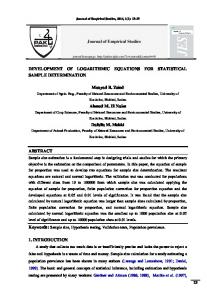
3.1.1. An Example: the Tricritical Ising Model To make things more demonstratic, let us introduce an example here: Following the Ising model, which constitutes the simplest unitary minimal model, the next one, 7 . namely M(5, 4), is the so-called Tricritical Ising Model with central charge 10 The dilute Ising model at its tricritical fixed point is defined like an ordinary Ising model, except that vacant sites are allowed and the number of spins on the lattice fluctuates. The configuration energy is X X E[σi , ti ] = − ti tj (K + δσi ,σj ) − µ ti , (3.1.3) hiji

i

where the variable ti = σi2 is 0 if site i is vacant and 1 otherwise. While K is the energy of a pair of unlike spins, K + 1 is the energy of a pair of like spins, respectively. The average number of occupied sites on the lattice is specified by the

21

3.1. Minimal Models chemical potential µ. The model is characterized as tricritical, since a critical point arises at some value dependent on β, K and µ, where three phases meet and coexist critically. Besides the identity operator (labeled as 1 in figure 3.1.1), there emerge five other scaling operators at this tricritical point: three energy- (labeled as , 0 and 00 in figure 3.1.1) and two spin-like operators (labeled as σ and σ 0 in figure 3.1.1), corresponding to the different highest weights in the Kaˇc table. Due to the symmetry property hr,s = hp0 −r,p−s

(3.1.4)

half the highest weights in the Kaˇc table are redundant.

6

4 # # 00

h3,1 =

r

u

3

σ0

h2,1 = u

2

0

3 2

7 16

h3,2 = u

σ

h2,2 = u

h3,3 =

3 5

u

1 10

# #

# u

h3,4#= 0

# # 3 h 80 # 2,3

#

u

=

3 80

h2,4 =

7 16

3 5

h1,4 =

3 2

u

# #

1 # h1,1 = 0 # h1,2 =

1

u # #

u

1

2

1 10

h1,3 = u

u

# # # 0 # 0

3

4

s

-

5

Figure 3.1.: The Kaˇc table for the minimal model M(5, 4) Note that the complete set of different highest weights of the Kac table 3.1.1 for 3 1 7 33 this minimal model, namely, in increasing order, h ∈ {0, 80 , 10 , 16 , 5 2 }, can be read off with the help of the vanishing curves in figure 2.3.1: Starting at the central 7 charge c = 10 and following the vertical line, the wanted h-values can be identified as the intersection points with the corresponding vanishing curves. Furthermore, this model is one of the few physically relevant theories that feature supersymmetry [FQS85]: The superconformal algebra or super-Virasoro algebra, a generalized Virasoro algebra, leads to pairs of fields and their corresponding superpartners, which are called superfields. Thus, the formulation of supersymmetric CFTs is possible in general.

22

Chapter 3. Bosonic Expressions

3.1.2. The Character of a Verma Module Since characters encode the physical spectrum with the information on the multiplicities of states in a highest weight module V , they play a crucial role in conformal field theory. The character χV is the holomorphic function on the complex upper half plane (τ ∈ C, Im(τ ) > 0), defined by c

χV (τ ) = TrV (q L0 − 24 )

(3.1.5)

with q = e2πiτ . With the generating function of the already mentioned partition function p(n) from (2.3.6) the character of a generic Verma module may be written as c q h− 24 χV (τ ) = (3.1.6) φ(q) Introducing the famous Dedekind η-function (see B.1 in the appendix) 1 24

η(τ ) ≡ q φ(q) = q

1 24

∞ Y

n=1

(1 − q n ) ,

(3.1.7)

the Virasoro character becomes 1−c

q h+ 24 χV (τ ) = η(τ )

(3.1.8)

3.1.3. Irreducible Modules As a consequence of the Kaˇc determinant formula (2.3.7), we now go into the structure of irreducible Verma modules, i.e. we describe the embedding structure of the reducible Verma modules, which in the end leads to the minimal character formula. Here we recall that only those representations with highest weights h are reducible if and only if the highest weights are parametrized by 0

hp,p r,s =

(pr − p0 s)2 − (p − p0 )2 4pp0

(3.1.9)

with the corresponding conformal charges cp,p0 = 1 − 6

(p − p0 )2 , pp0

(3.1.10)

for some non-negative integers r, s ≥ 1. 0 A reducible Verma module with highest weight hp,p r,s , denoted by Vr,s in this section, has its first singular vector at level l = rs according to (2.3.7). An appearance of another singular vector at level (p0 −r)(p−s) follows from the symmetry property (3.1.4). From (3.1.9) one can derive the identities hr,s + rs = hp0 +r,p−s = hp0 −r,p+s hr,s + (p − r)(p − s) = hr,2p−s = h2p0 −r,s , 0

(3.1.11) (3.1.12)

23

3.1. Minimal Models which state that the two singular vectors that are contained in Vr,s are themselves highest weights of degenerate Verma modules, since they fit in (2.3.7). Furthermore, these new submodules give rise to the same structure, i.e. they also contain singular vectors, which in turn are highest weight vectors for modules that again contain singular vectors and so on. This structure is suggested graphically in the following figure 3.2. .. . A A A A A A

A A A A A A A A A A A A A A A A A A A A A A A A A A A A A A A A A A A A A A A A A A A A A A A A A A A A A A A A level (p0 − r)(p − s) A A level rs AA A A A A A A

Figure 3.2.: The interlocking of Verma modules The first inclusion of submodules can hence be written as Vp0 +r,p−s ∪ Vr,2p−s ⊂ Vr,s

(3.1.13)

If we just factor out Vr,s by the union of these two submodules, we would subtract too much, since the submodules in turn contain singular vectors, which are highest weights of new submodules. Thus, the irreducible Virasoro module Mr,s is obtained after the sum of these submodules has been factored out, namely Mr,s =

Vr,s . Vp0 +r,p−s + Vr,2p−s

(3.1.14)

Keeping in mind the mentioned embedding structure and taking again advantage of some symmetry properties, the sum Vp0 +r,p−s + Vr,2p−s can be taken into the form of a quotient Vp0 +r,p−s ∪ Vr,2p−s Vp0 +r,p−s + Vr,2p−s = , (3.1.15) V2p0 +r,s + Vr,2p+s which leads, by iterating this expression, to the infinite embedding structure of the Verma module Vr,s with 1 ≤ r < p0 , 1 ≤ s < p, whose form is depicted in the following figure 3.3. Finally, we obtain the irreducible Virasoro module Mr,s , which

24

Chapter 3. Bosonic Expressions (p0 + r, p − s)

(r, s)

K A A

A A

K AA A

A A

(2p0 + r, s) r r r

A A A A A A A

A

(r, 2p − s)

(r, 2p + s)

K AA A

A A

(kp0 + r, (−1)k s + [1 − (−1)k ] 2p ) r r r

A A A A A A A r r r

(r, kp + (−1)k s + [1 − (−1)k ] p2 ) r r r 0

p,p Figure 3.3.: The infinite embedding structure for a Verma module Vr,s .

is given as an alternating sum that mirrors the successive subtractions and additions of the diverse submodules:

Mr,s = Vr,s − (Vp0 +r,p−s ∪ Vr,2p−s) + (V2p0 +r,s ∪ Vr,2p+s ) − · · · .

(3.1.16)

This alternating structure, i.e. the first subtraction is too large, so you have to add the wrongly subtracted submodules and so on, will turn out to be of great importance in later chapters, since it is the signature of so-called bosonic character expressions.

3.1.4. Minimal Characters

With the results of the last two sections we now have all ingredients to write the character of the irreducible Verma module Mr,s in an extremely simple form. Principally, we just have to follow the corresponding embedding chain, e.g. the one for

25

3.1. Minimal Models minimal models in figure 3.3.1 : 0 χp,p r,s

= = = = =

q

1−c 24

q

1−c 24

q hr,s − q hr,−s − q hr,2p−s + q hr,s+2p + q hr,s−2p − . . .

η

−

η q

n=0 ∞ X

1−c 24

η q

n=−∞

1−c 24

η q

1 = η

∞ X

∞ X

q hr,−s−2pn −

∞ X

q hr,2pn−s +

n=1

q hr,s+2pn − q hr,2pn−s q

n=−∞

1−c 24

q η

c−1 24

∞ X

∞ X

q

(pr−p0 s−2pp0 n)2 4pp0

n=−∞

q

(2kn+λ)2 4k

n=−∞

−q

(2kn+λ0 )2 4k

−q

−q

!

q hr,s+2pn +

n=0

!

(pr−p0 (s+2pn))2 −(p−p0 )2 4pp0

∞ X

∞ X n=1

(pr−p0 (−s+2pn))2 −(p−p0 )2 4pp0

(pr+p0 s−2pp0 n)2 4pp0

!

1 = (Θλ,k − Θλ0 ,k ) , η

q hr,s−2pn

!

!

(3.1.17)

where we have obtained the important Θ-functions by setting k = pp0 , λ = pr − p0 s and λ0 = pr + p0 s (cf. section B.2 in the appendix). Since the range for the r- and s-values is set by r ∈ {1, 2, 3} and s ∈ {1, 2, 3, 4}, six different characters for the in section 3.1.1 introduced Tricritical Ising Model arise, which can now be written as 1 1 (Θ1,20 − Θ9,20 ) = (Θ−1,20 − Θ31,20 ) η η 1 1 = (Θ−3,20 − Θ13,20 ) = (Θ3,20 − Θ27,20 ) η η 1 1 (Θ7,20 − Θ23,20 ) = (Θ−7,20 − Θ17,20 ) = η η 1 1 = (Θ−11,20 − Θ21,20 ) = (Θ11,20 − Θ19,20 ) η η 1 1 (Θ2,20 − Θ18,20 ) = (Θ−2,20 − Θ22,20 ) = η η 1 1 = (Θ−6,20 − Θ26,20 ) = (Θ6,20 − Θ14,20 ) . η η

5,4 χ5,4 1,1 =χ3,4 =

(3.1.18)

5,4 χ5,4 1,2 =χ3,3

(3.1.19)

5,4 χ5,4 1,3 =χ3,2 5,4 χ5,4 1,4 =χ3,1 5,4 χ5,4 2,2 =χ2,3 5,4 χ5,4 2,4 =χ2,1

(3.1.20) (3.1.21) (3.1.22) (3.1.23)

Their corresponding q-series expansions, which are normalized to one by dividing 1

For purposes of clarity, the dependence on τ or q, respectively, is omitted here and in the following as well as in later chapters if this cannot lead to confusion.

26

Chapter 3. Bosonic Expressions λ2

out the offset given by q 4k , are 1

5,4 − 80 χ5,4 (1 + q 2 + q 3 + 2q 4 + 2q 5 + 4q 6 1,1 = χ3,4 = q

+ 4q 7 + 7q 8 + 8q 9 + 12q 10 + 14q 11 + 20q 12 + 23q 13 + O(q 14 )) 5,4 χ5,4 1,2 = χ3,3 = q

9 − 80

(1 + q + q 2 + 2q 3 + 3q 4 + 4q 5 + 6q 6

+ 8q 7 + 11q 8 + 14q 9 + 19q 10 + 24q 11 + 32q 12 + 40q 13 + O(q 14 )) 5,4 χ5,4 1,3 = χ3,2 = q

49 − 80

=

χ5,4 3,1 7

=q

− 121 80

5,4 χ5,4 2,2 = χ2,3 = q

5,4 χ5,4 2,4 = χ2,1 = q

(3.1.27)

(1 + q + 2q 2 + 3q 3 + 4q 4 + 6q 5 + 8q 6

+ 11q 7 + 15q 8 + 20q 9 + 26q 10 + 34q 11 + 44q 12 + 56q 13 + O(q 14 )) 9 − 20

(3.1.26)

(1 + q + 2q 2 + 2q 3 + 3q 4 + 4q 5 + 6q 6

+ 7q + 10q 8 + 13q 9 + 17q 10 + 21q 11 + 28q 12 + 34q 13 + O(q 14 )) 1 − 20

(3.1.25)

(1 + q + 2q 2 + 2q 3 + 4q 4 + 5q 5 + 7q 6

+ 9q 7 + 13q 8 + 16q 9 + 22q 10 + 27q 11 + 36q 12 + 45q 13 + O(q 14 )) χ5,4 1,4

(3.1.24)

(3.1.28)

(1 + q + q 2 + 2q 3 + 3q 4 + 4q 5 + 6q 6

+ 8q 7 + 10q 8 + 14q 9 + 18q 10 + 23q 11 + 30q 12 + 38q 13 + O(q 14 )) . Comparing these q-expansions with the expansion of

1 , φ(q)

(3.1.29)

namely

1 1 1 = 1 + q + 2q 2 + 3q 3 + 5q 4 + 7q 5 =Q = n φ(q) (q) (1 − q ) ∞ n≥1

+11q 6 + 15q 7 + 22q 8 + 30q 9 + 42q 10 + 56q 11 + 77q 12 + 101q 13 + · · · ,

(3.1.30)

one can easily verify that the first two singular vectors occur at level rs and at level (4 − r)(5 − s), respectively (cf. the q-series expansions of the c = −2 model in section D in the appendix).

3.2. Logarithmic Models After it was noted in [Kni87] that correlation functions may also exhibit logarithmic divergences, the concept of a CFT with logarithmic singularities occuring in the correlation functions was introduced by Gurarie [Gur93]. The main difference to ordinary rational CFTs such as the minimal models is that the representations of the chiral symmetry algebra may be indecomposable. But otherwise the LCFTs, especially the here explicitly considered cp,1 series, are very close to rationality. Almost all important structures, basic notions and tools of (rational) CFTs, such as null vectors, (bosonic) character functions, partition functions, fusion rules, modular invariance, OPEs, have been generalized by now. So nowadays the understanding of of LCFTs is almost at the same level as the one about (rational) conformal field theories. Furthermore, there exists a huge number of applications for LCFTs, which include topics like two-dimensional conformal turbulence, the fractional quantum Hall effect (see chapter 1) and AdS/CFT-correspondence.

27

3.2. Logarithmic Models

3.2.1. W-Algebras In the following, we want to concern extended conformal symmetry algebras, the so-called W-algebras as introduced by [Zam85]. As can be comprehended in [BFK+ 90], W-algebras describe the operator product expansion (cf. (2.2.12)) of conformally invariant local chiral fields. While the singular part of such an OPE yields a Lie bracket structure for the Fourier modes of the fields, the regular part provides an operation of forming normal ordered products. A W-algebra is generated by a finite set of simple, i.e. they are not composed from others by normal ordering, primary fields φ0 , φ1 , . . . , φn including the identity. Hence, it is denoted by W(2, d1 , . . . , dn ), where the di = h(φi ) stand for the conformal dimensions and d0 = 2 for the Virasoro field instead of the identity field. So, for example, the W-algebra, which is generated by three primary fields, which all have conformal dimension three, is denoted by W(2, 3, 3, 3). This is in fact the most prominent candidate and therefore should bother us in the next section. Other examples are the super-Virasoro algebra (cf. section 3.1.1) W(2, 23 ), the direct sum of two Virasoro algebras W(2, 2) or the Casimir algebras of the affine Kaˇc-Moody algebras W(2, 3), W(2, 4) and W(2, 6) [Flo94].

3.2.2. The W(2, 3, 3, 3)-Algebra Let us only consider the c( 2, 1) model of the cp,1 series in detail here, since it should be sufficient to understand the basic ideas. The Virasoro theory at c = −2 is not rational – it has infinitely many representations – with respect to the Virasoro algebra, but it is rational with respect to an extended chiral symmetry algebra in the sense that it only possesses finitely many indecomposable representations that close under fusion [Gab03]2 . At first, those extensions of the Virasoro algebra, resulting in a multiplet structure of fields with integer or half-integer spin – in particular the triplet structure, which will be of interest to us in the next sections – were studied in [Kau91]. Let us recall that the possible highest weights are given through the extended Kaˇc table, which is displayed in figure 3.4, by h2,1 r,s =

(2r − s)2 − 1 8

(3.2.1)

and hence especially h3,1 = 3, which plays a decisive role for the following symmetry algebra extension. The triplet W-algebra is the extension of the Virasoro theory by a triplet of fields W i with h = h3,1 = 3. Here, an important role is played by the screening charges Q, which are given by I Q=

dzVα+ (z)

(3.2.2)

with the vertex operator Vα+ (z) that arises in the context of the free field construction in [Kau91]. These screening charges Q are actually responsible for the triplet 2

Note the definition of quasi-rationality in this context: [Nah96, Flo03].

28


6

3

r

h2,1 = 1

h2,2 =

u

2

u

3 8

h2,3 = 0 u

1 h2,4 = − h2,4 = 0 8

u

u

h1,1 = 0 u

1

1 h1,3 = 0 h1,2 = − 8

u

u

2

3

h1,4 = u

3 8

h1,4 = 1 u

0 0

1

4

5

s

-

6

Figure 3.4.: The extended Kaˇc table for the c = −2 model structure, which is obtained by repeated application of Q on the field φ3,1 W i = Qi φ3,1 .

(3.2.3)

This leads eventually to three fields with SO(3) structure, which, together with the energy-momentum tensor, generate the desired W(2, 2p − 1.2p − 1, 2p − 1)-algebra. As mentioned above, we are interested in the case of p = 2 here: Expressed in an orthonormal basis, i.e. the metric gab and the structure constants fcab of su(2) take the form δ ab and iabc , respectively, the commutation relations for the corresponding modes Wna of the fields and the modes Ln of the energymomentum tensor then read 1 [Ln , Lm ] = (n − m)Ln+m − n(n2 − 1)δn+m,0 , 6 a a [Ln , Wm ] = (2n − m)Wn+m , 1 a b ab [Wn , Wm ] = δ 2(n − m)Λn+m + (n − m)(2n2 + 2m2 − nm − 8)Ln+m 20 1 2 2 − n(n − 1)(n − 4)δm+n,0 120 12 c 5 2 2 c abc (2n + 2m − 3nm − 4)Wn+m + Vn+m , + i 14 15

(3.2.4) (3.2.5) (3.2.6) (3.2.7) (3.2.8)

3 2 ∂ Lm and Vma =: with the normal ordered quasi-primary fields Λm =: L2m : − 10 3 2 Lm Wma : − 14 ∂ Wma (a, b, c ∈ {1, 2, 3} and n, m ∈ Z). The existence of singular vectors in the vacuum representation leads to constraints for the allowed representations – i.e. their zero modes have to vanish on any highest weight state ψ in order

29

3.2. Logarithmic Models to get a physical spectrum of L0 , which is bounded from below – of the following form: a b ab 1 2 abc 1 c W0 W0 − δ L0 (8L0 + 1) − i (6L0 − 1)W0 ψ = 0 (3.2.9) 9 5 This constraint governs the highest weight representations to have an su(2) structure, since 2 [W0a , W0b ] = (6h − 1)iabc W0c , (3.2.10) 5 which follows from (3.2.9), is a rescaled version of the su(2) algebra. The irreducible representations of these zero modes can be labeledPas is customary after rescaling: j(j + 1) is the eigenvalue of the Casimir operator 3i=1 (W0i )2 and m the eigenvalue of W03 . Furthermore, (3.2.9) leads to the relation j(j + 1) = 3m2 ,

(3.2.11)

since the action of W0a W0a is the same as W0b W0b on highest weight states. Evaluating this restriction, we have finally arrived at the allowed representations [EHH93, GK96b]: j = 0: Two singlet representations – V0 at h = 0

– V− 1 at h = − 18 8

j = 21 : Two doublet representations – V1 at h = 1 – V 3 at h = 8

3 8

.

Those readers, who find this analysis to be too physical, are referred to [Zhu96]. Analyzing the fusion products (see e.g. [Ver88] for the constitutional fusion rules in the context of modular invariance and [Knu06] for recent developments concerning fusion with regard to LCFT) for these four irreducible representations [GK96b], we find two generalized highest weight representations R0 and R1 . Their sketched structures can be found in the figures 3.5 and 3.6. Here, each dot in the bottom row stands for the irreducible representation V0 and each one in the top row for V1 . The action of the triplet algebra is indicated by the arrows. R0 is generated from a highest weight vector ω of h = 0, which is a singlet under su(2), forming a Jordan cell for L0 with Ω, i.e. L0 ω = Ω. The four states L−1 ω a and W−1 ω form two doublets and are therefore denoted by Ψ1 and Ψ2 . Furthermore, note that R0 is an extension of the vacuum representation. R1 is generated from a doublet φ± of weight h = 1, denoted by φ in the corresponding figure. It has two ground states ξ ± at h = 0 and another doublet ψ ± at h = 1, denoted by ψ in the corresponding figure, forming L0 Jordan cells with φ± . Furthermore, R1 is not a highest weight representation. The relations, which define the action of the Virasoro and the triplet algebra in both cases, are given in detail

30


Ψ1

Ψ2

zz HH I @ @ HH HH @ H @ H H HH@ @ HH @ H z z zz Y H H

Ω

L0

h=1

h=0

ω

Figure 3.5.: The indecomposable representation R0 ψ

zz k QQ

φ

Q

Q

Q

Q

Q

Q

Q

Q

Q + zz

ξ

+

ξ

−

zz

h=1

h=0 .

Figure 3.6.: The indecomposable representation R1 in [GK96b]. Both of these representations are indecomposable. The set of these six mentioned representations closes under fusion. In the following chapters we do not distinguish between R0 and R1 , since they are isomorphic to each other. Finally, note the interesting fact that the occurring partition function of the full theory is actually the same as that of a free boson compactified on a circle of radius √ 2 [Gin88b].

3.2.3. The Indecomposable Representation As already mentioned, LCFTs are intimately connected with the existence of indecomposable representations. A Jordan cell of states takes the place of a unique highest weight state in a representation module. These new ’highest weight states’ are linked by the action of a non-diagonalizable operator, which might be any generator, but is at last mainly the energy-momentum tensor, of the (extended) chiral symmetry algebra. To illustrate the Jordan cell structure, let us assume that there exist two operators Φ and Ψ with an equivalent set of quantum numbers with respect

31

3.2. Logarithmic Models to the maximally extended chiral symmetry algebra, the same conformal weight h included. As a consequence, the L0 operator can no longer be diagonalized and thus takes the form Φ h 0 Φ . (3.2.12) = L0 Ψ 1 h Ψ Let us now go into more detail with regard to the structure of an indecomposable representation, following [GK96a], since it is not only a central aspect for the c = −2 model, but also for an LCFT in general. To make things clear, we choose a representation similar to R0 , which we call R here, since R1 is not a highest weight representation. As it is the case for R0 , it is generated from a highest weight state ω satisfying L0 ω = Ω ,

L0 Ω = 0 ,

Ln ω = 0 for n > 0

(3.2.13)

by the action of the Virasoro algebra, i.e. no extensions are considered here. The state χ = L−1 Ω is a null-state of R, but ξ = L−1 ω is not singular, since L1 L−1 ω = [L1 , L−1 ]ω = 2L0 ω = 2Ω. The following figure 3.7 shows a sketch of R. e

I @ @

eχ

I @ @

@

@

@

@

uξ

I @ @

@

@

u

Ω

h=1 @

@ @

u

h=0

ω

Figure 3.7.: The indecomposable representation R Here each filled dot denotes a state of the representation space, and the unfilled dots correspond to singular vectors. A −→ B indicates that B is in the image of A under the action of the Virasoro algebra. Letting the Virasoro modes act on Ω, the complete set of the obtained states shapes up as a subrepresentation Rsub of R being isomorphic to the vacuum representation. This observation shows that R cannot be irreducible. On the other hand, R is also not completely reducible: We cannot write R as a direct sum of its submodules, since we cannot find a complementary subspace to Rsub that is a representation by itself. Hence, R is called an indecomposable (but reducible) representation.

3.2.4. Characters of the Triplet Algebras W(2, 2p − 1, 2p − 1, 2p − 1) 0

A minimal model with central charge c = cp,p0 admits highest weights hp,p r,s (cf. 0 (3.1.9)) with 1 ≤ r < p and 1 ≤ s < p.

32

Chapter 3. Bosonic Expressions In contrast, the h-values of all 3p − 1 inequivalent representations for the LCFT models with cp,1 and chiral symmetry algebra W(2, 2p − 1, 2p − 1, 2p − 1) can be read off the extended conformal grid of the augmented minimal model [Flo97, EF06], corresponding formally to central charge c3p,3 . For example, in the case p = 2 and c2,1 = −2, the only possible highest weights are h ∈ {− 81 , 0, 83 , 1}, where h = 0 corresponds to two inequivalent representations [GK96b]. Here, (3.2.9) and a null vector constraint can be transformed to obtain the condition 0 = L20 (8L0 + 1)(8L0 − 3)(L0 − 1)ψ ,

(3.2.14)

ψ being any highest weight state, which states that L0 has to take exactly those h-values, which we just read off the extended conformal grid. In addition, note that (3.2.14) in general allows a logarithmic highest weight representation, since we only have to claim that L20 = 0, but not necessarily that L0 = 0. In particular, a twodimensional space of highest weight states similar to (3.2.12) copes with (3.2.14). In general, the possible highest weights for a given W-algebra can be determined explicitely with the help of Jacobi identities and constraints on the singular vectors. In comparison to the singlet algebra W(2, 2p − 1), which is too small to obtain a rational cp,1 model, the triplet algebra now serves as its maximally extended symmetry algebra. The way to get the W-algebra characters is to sum up appropriate subsets of Virasoro characters of degenerate highest weight representations, which is in conjunction with the fact that many properties are only defined modulo Z for characters. One also has to keep in mind that only those highest weights are permitted which differ by integers and has to take care of multiplicities caused by the su(2) symmetry among the triplet of chiral fields of conformal weight 2p − 1. The multiplicity of the Virasoro highest weight representation on |h2k+1,1 i turns out to be 2k + 1. For k = 1, i.e. h3,1 = 2p − 1, the dimension three matches the desired triplet structure. Fortunately, the structure for these representations appears even simpler than the one for minimal models: Due to the classification of Feigin and Fuks [FF82], there exists exactly one null vector, which leads to the following form for the Virasoro characters: χVir 2k+1,1 =

1 (q h2k+1,1 − q h2k+1,−1 ) . η(q)

(3.2.15)

Summarizing all the mentioned points, the vacuum representation of the W-algebra is then the Hilbert space

W H|0i =

M

Vir (2k + 1)H|h . 2k+1,1 i

(3.2.16)

k∈Z+

33

3.2. Logarithmic Models So, the vacuum character is [Flo03] X χW = (2k + 1)χVir 0 2k+1,1 k∈Z+

X

q (1−c)/24 = η(q)

k≥0

q (1−c)/24 = η(q) = =

q

η(q)

(2k + 1)q h2k+1,1 +

k≥0

(1−p)2 /4p

η(q) 1 X

X

(2k + 1)q h2k+1,1 −

X

X

(2k + 1)q h−(2k+1),1

k≥0

X

(−2k + 1)q h−2k+1,1

k≥1

(2k + 1)q

!

!

(1−(2k+1)p)2 −(1−p)2 4p

k∈Z

(2k + 1)q (

2pk+(p−1))2 4p

k∈Z

1 = ((∂Θ)p−1,p (τ ) + Θp−1,p (τ )) . pη(τ )

(3.2.17)

In the last line the character has been rewritten in terms of Θ-functions and affine Θ-functions (see sections B.2 and B.3 in the appendix). Θ are modular forms of weight 0, we meet Although the functions Λλ,k = λ,k η a problem with the terms, where the affine Θ-functions are involved: (∂Λ)λ,k = (∂Θ)λ,k have weight 1. To solve the problem, a factor η 3 would be necessary in the η denominator like it is the case for the characters of the affine Kac-Moody algebras [ equivalent to A(1) (cf. section 5.4). su(2) k The Complete Set of the Bosonic cp,1 Characters Analyzing the action of the triplet algebras on the degenerate Virasoro representations [GK96b, Flo96] as well as the modular transformation properties of the vacuum character allows to find a complete set of character functions for the cp,1 models that is closed under modular transformations [Flo97]: χ0,p = χp,p = χ+ λ,p = χ− λ,p = χ˜+ λ,p = χ˜− λ,p =

34

Θ0,p η Θp,p η (p − λ)Θλ,p + (∂Θ)λ,p pη λΘλ,p − (∂Θ)λ,p pη Θλ,p + iαλ(∇Θ)λ,p η Θλ,p − iα(p − λ)(∇Θ)λ,p η

representation to

hp,1 1,p

(3.2.18)

hp,1 1,2p

(3.2.19)

hp,1 1,p−λ

(3.2.20)

hp,1 1,3p−λ

(3.2.21)

hp,1 1,p+λ

(3.2.22)

hp,1 1,p+λ ,

(3.2.23)

Chapter 3. Bosonic Expressions where 0 < λ < p, k = pp0 = p, λ = pr − p0 s = pr − s. The following definitions are listed for convenience (cf. sections B.2, B.3 and B.1 in the appendix): The Jacobi-Riemann Θ-function is defined as X (2kn+λ)2 Θλ,k (τ ) = q 4k , (3.2.24) n∈Z

the affine Θ-function defined as (∂Θ)λ,k (τ ) =

X (2kn+λ)2 (2kn + λ)q 4k

(3.2.25)

n∈Z

and the Dedekind η-function defined as η(q) = q 1/24 (q)∞ . Θ

(3.2.26)

(τ )

λ,k Here, q = e2πiτ , τ ∈ h (upper half-plane). η(τ is a modular form of weight zero ) with respect to the generators T : τ 7→ τ + 1 and S : τ 7→ − τ1 of the modular (∂Θ) (τ ) group P SL(2, Z). But since η(τλ,k) is a modular form of weight one with respect to S, some of the above character functions are of inhomogeneous modular weight, thus leading to S-matrices with τ -dependent coefficients. However, adding

(∇Θ)λ,k (τ ) =

(2kn+λ)2 log q X (2kn + λ)q 4k , 2πi n∈Z

(3.2.27)

one finds a closed finite dimensional representation of the modular group with constant S-matrix coefficients. Note that (3.2.22) and (3.2.23) are not characters of representations in the usual sense. Actually, these are regularized character functions and the α-dependent part has an interpretation as torus vacuum amplitudes [FG06]. In the limit α → 0, they become the characters of the full reducible but indecomposable representations. The q-series expansions of the c2,1 model are displayed in section D in the appendix.

3.3. Parabolic Models To conclude this chapter, let us come to the parabolic models, which have been quoted in section 3.3.

3.3.1. Characters of the W(2, 3k)-Algebras Choosing k as integer or half-integer, then all allowed highest weights are given by hr,r = (r 2 − 1)k h−r,r = (r 2 − 1)k + r 2 ,

(3.3.1) (3.3.2)

35

3.3. Parabolic Models Z

likewise being integer or half-integer. Allowing only odd r- values, choosing k ∈ ≥0 4 is also possible. Thus, all requirements are fulfiled to guarantee a local system of chiral BRST-invariant screened vertex operators [Flo94]. Here the locality also constricts the fusion rules of the chiral algebra: The corresponding highest weights may only differ by integer or half-integer values again [God89]. Z A consequence of the modular properties is that choosing k ∈ ≥0 is the only way 4 to obtain rational conformal field theories from parabolic models. Z An interesting algebra is given for c = 1 − 24k with k ∈ ≥0 : the W(2, 3k)2 algebra. It is constructed from chiral vertex operators of a free field representation. Comparing the commutator of the modes of two such operators, one can show that this algebra has indeed only two generators: The Virasoro field and the field with conformal dimension h2,2 = 3k, as can be verified by using (3.3.1), with its modes, which both form a Lie algebraic structure. This theory is just mentioned marginally here, since we only want to draw the reader’s attention to the corresponding character expressions. For details we refer to [Flo93, Flo94]. The relevant representations and their characters of the bosonic W(2, 3k)-algebras 3 are the following: 1 χW 0 = (Λ0,k (τ ) − Λ0,k+1 (τ )) 2 χW 1

= Λ1,k (τ )

(vacuum representation) (3.3.3) (3.3.4)

.. . χW k,+

χW k−1 = Λk−1,k (τ ) 1 = χW k,− = Λk,k (τ ) 2 1 χW k+1 = (Λ0,k (τ ) + Λ0,k+1 (τ )) 2 χW −1

= Λ1,k+1 (τ )

(3.3.5) (degenerate representation) (3.3.6) (representation to hmin ) (3.3.7) (3.3.8)

.. . χW −k−1,+

3

χW −k = Λk,k+1 (τ ) 1 = χW −k−1,− = Λk+1,k+1 (τ ) 2

(3.3.9) (degenerate representation) (3.3.10)

Only the even sectors are considered here: For the odd sectors, a W(2, 8k)-algebra can be obtained in an analogous manner.

36

4. A Gateway to the Other Side The Rogers-Ramanujan identities provide one of the most fascinating chapters in the history of partitions. The story began with the discovery of the Indian genius S. Ramanujan by G. H. Hardy. In Ramanujan’s first letter to Hardy from 1913, two outstanding examples on continued fractions, s  √ √ 1 5+ 5 5 + 1  2π = (4.0.1) e5 − −2π 2 2 e 1+ e−4π 1+ e−6π 1+ 1+... and 1−

e 1+

−π

e

−2π

s

=

√

5− 5 − 2

√



5 − 1 π e5 , 2

(4.0.2)

e−3π 1+... were commented by Hardy in his article [Har37]: ”[These formulas] defeated me completely. I had never seen anything in the least like them before. A single look at them is enough to show that they could only be written down by a mathematician of the highest class. They must be true because, if they were not true, no one would have had the imagination to invent them.” Let us relate these continued fractions to the Rogers-Ramanujan identities now: We start with a linear second-order q-difference equation 1 1−

F (x) = F (xq) + xqF (xq 2 ) , where the function F (x) is analytic in x at 0 and F (0) = 1. Setting we get xq c(x, q) = 1 + c(xq, q) xq 2 c(xq, q) = 1 + c(xq 2 , q) xq 3 c(xq 2 , q) = 1 + c(xq 3 , q) .. .. . . . 1

(4.0.3) F (x) F (xq)

= c(x, q), (4.0.4) (4.0.5) (4.0.6)

see [FS93b] for some additional information on q-difference equations in the context of Virasoro characters

37

Plugging these expressions into each other, we have already obtained a generalized version of Ramanujan’s continued fraction, namely c(x, q) = 1 +

xq . xq 2 1+ xq 3 1+ xq 4 1+ 1+···

(4.0.7)

Thus, it can be easily checked that the two theorems at the beginning of this chapter are precisely those evaluations of c(1, e−2π ) and c(1, −e−π ). Furthermore, we can expand F(x) in a power series X F (x) = An (q)xn , (4.0.8) n≥0

which yields, after being substituted in (4.0.3) and by comparing coefficients of xn , An (q) = q n An (q) + q 2n−1 An−1 (q) .

(4.0.9)

Successively using this expression, we can calculate q (2n−1)+(2n−3) q 2n−1 A (q) = An−2 (q) n−1 1 − qn (1 − q n )(1 − q n−1 ) 2 q 1+3+···+(2n−1) qn =··· = A0 (q) = . (q)n (q)n

An (q) =

So finally we get Fx (q) =

2 ∞ X xn q n

n=0

(q)n

.

(4.0.10) (4.0.11)

(4.0.12)

Applying this power series, F1 (q) and Fq (q) can now be written as infinite products2 : F1 (q) =1 + =

∞ Y

n=1

q q4 q9 + + +··· 1 − q (1 − q)(1 − q 2 ) (1 − q)(1 − q 2 )(1 − q 3 ) 1

(1 −

q 5n−1 )(1

− q 5n−4 )

(4.0.13) (4.0.14)

and Fq (q) =1 + = 2

∞ Y

q2 q6 q 12 + + +··· 1 − q (1 − q)(1 − q 2 ) (1 − q)(1 − q 2 )(1 − q 3 )

1 . (1 − q 5n−2 )(1 − q 5n−3 ) n=1

A proof can be found in [And84a]

38

(4.0.15) (4.0.16)

Chapter 4. A Gateway to the Other Side With both of these last results, we are now able to write c(1, q) in an infinite product. And in particular, F1 (q) and Fq (q) match the infinite product representations of the famous Rogers-Schur-Ramanujan identities (4.2.1) and (4.2.2), respectively, which will ultimately lead us to the desired fermionic character expressions. Note that F1 (q) and Fq (q) are derived that explicitly here, since we will encounter them again in the context of q-hypergeometric series and modular forms in chapter 6. But let us first of all put these identities in perspective with respect to the interpretation in terms of partitions, based on a generalization by Gordon.

4.1. Gordon’s Generalization The following theorem in terms of partitions is due to B. Gordon: Let Bk,i (n) denote the number of partitions of n of the form (b1 b2 . . . bs ), where bj − bj+k−1 ≥ 2, and at most i − 1 of the bj equal 1. Let Ak,i (n) denote the number of partitions of n into parts 6≡ 0, ±i (mod 2k + 1). Then Ak,i (n) = Bk,i (n) for all n. Its most celebrated corollaries are the two Rogers-Ramanujan identities – at first stated in terms of partitions here: The first identity (k = i = 2). The partitions of an integer n in which the difference between any two parts is at least 2 are equinumerous with the partitions of n into parts ≡ 1 (mod 5) or ≡ 4 (mod 5) The second identity (k = i + 1 = 2). The partitions of an integer n in which each part exceeds 1 and the difference between any two parts is at least 2 are equinumerous with the partitions of n into parts ≡ 2 (mod 5) or ≡ 3 (mod 5). Its analytic counterpart from [And74] applies for 1 ≤ i ≤ k, k ≥ 2, |q| < 1: X

n1 ,n2 ,...,nk−1

2

2

2

q N1 +N2 +···+Nk−1 +Ni +Ni+1 +···+Nk−1 = (q) (q) · · · (q) n n n 1 2 k−1 ≥0

n6≡0,±i

∞ Y

(1−q n )−1 , (4.1.1)

n=1 (mod 2k+1)

with Nj = nj +nj+1 +· · ·+nk−1 . This identity, one of the so-called Andrews-Gordon identities, introduces a sum over multi-indices and thus plays an important role on the way to fermionic character expressions and therewith to dilogarithm identities [NRT93]. Furthermore, each of the classical identities of Rogers-Ramanujan type can be used to yield further multiple sum series identities: It is shown in [And84b] how the Bailey chain is used to achieve this.

39

4.2. The Connection to Characters

4.2. The Connection to Characters The famous Rogers-(Schur-3 )Ramanujan identities [Rog94, Sch17, RR19] 2 ∞ ∞ X Y qn 1 = 5n−1 (q)n n=1 (1 − q )(1 − q 5n−4 ) n=0

and

2 ∞ X q n +n

(q)n

n=0

=

(4.2.1)

∞ Y

1 , (1 − q 5n−2 )(1 − q 5n−3 ) n=1

(4.2.2)

with the q-Pochhammer symbol defined as (see also A.1 in the appendix) (q)n =

n Y i=1

(1 − q i ) and per definition (q)0 = 1 and (q)∞ = lim (q)n , (4.2.3) n→∞

first of all built a bridge between bosonic and fermionic representations for a CFT character. In particular, these identities coincide with the two characters of the M(5, 2) minimal model [Fis78, Car85] (normalized to 1 at q 0 ). By using Jacobi’s triple product identity, which is stated for z 6= 0, |q| < 1 by ∞ X

n n2

z q

=

n=−∞

∞ Y

n=0

(1 − q 2n+2 )(1 + zq 2n+1 )(1 + z −1 q 2n+1 ) ,

(4.2.4)

the r.h.s.’s of (4.2.1) and (4.2.2) can be transformed to give two simple examples of what is called a bosonic-fermionic q-series identity, namely

and

2 ∞ ∞ X 1 X n(10n+1) qn = (q − q (5n+2)(2n+1) ) (q) (q) n ∞ n=−∞ n=0 2 ∞ X q n +n

n=0

(q)n

∞ 1 X n(10n+3) (q − q (5n+1)(2n+1) ) . = (q)∞ n=−∞

(4.2.5)

(4.2.6)

By the way, Jacobi’s triple product identity is a direct consequence of a corollary due to Euler (see e.g. [And84a]), which is defined for |t| < 1, |q| < 1 by ∞ ∞ X Y tn 1+ = (1 − tq n )−1 , (q)n n=0 n=1

1+

∞ n 1 n(n−1) X t q2 n=1

(q)n

=

∞ Y

(1 + tq n ) .

(4.2.7) (4.2.8)

n=0

Since we have already found a way of generalizing the bosonic sides of the identity to all known minimal models in section 3.1.4, the next step is now to clear the way for the generalization of the fermionic sides for all minimal models. Before we conclude this chapter, we touch on two important subjects with respect to the Rogers-Ramanujan identities: the physical background and the proof of new identities relating the bosonic and the fermionic sides of a character. 3

Schur is often omitted both in the literature and here as well.

40

Chapter 4. A Gateway to the Other Side

4.3. The Physical Background The occurrence of these bosonic-fermionic q-series identities is a peculiarity in twodimensional conformal field theory, i.e. there exists only one space dimension. In general, the nature of bosons and fermions is quite distinct in three space dimensions, regardless of whether the particles are expressed in terms of commutation and anti-commutation relations or through their spectra4 . Nevertheless, the fact that they are related in two dimensions provokes to the assumption that there exists a Bose-Fermi correspondence for every conformal field theory in question, i.e. all CFT characters can be written in two different sum representations, generalizing the Rogers-Schur-Ramanujan Identities. In particular, this assumption is supported by Nahm’s conjecture (cf. section 6.2). To confront the bosonic side with the fermionic side, let us summarize the most important facts here: As mentioned, the so-called bosonic expressions on the r.h.s.’s of (4.2.5) and (4.2.6), respectively, correspond to two special cases of the general character formula for minimal models M(p, p0 ) [RC84] 0

c

p,p0

0

−hr,s p,p 24 χ ˆp,p χr,s = r,s = q

∞ 1 X n(npp0 +pr−p0 s) 0 (q − q (np+s)(np +r) ) (q)∞ n=−∞

(4.3.1) 0

p,p p,p with χˆp,p r,s being the normalized character. The known symmetry χr,s = χp0 −r,p−s follows from (3.1.4). Since (4.3.1) is computed by eliminating null states from the Hilbert space of a free chiral boson [FF83], it is referred to as bosonic form. Its signature is the alternating sign, which reflects the subtraction of null vectors. The factor (q)∞ keeps track of the free action of the Virasoro ’raising’ modes. Furthermore, it can be expressed in terms of Θ-functions (see (B.2) in the appendix), which directly point out the modular transformation properties of the character. In contrast, the fermionic sum representation possesses a remarkable interpretation in terms of quasi-particles for the states, obeying Pauli’s exclusion principle (see chapter 7). The bosonic representations are in general unique, whereas there is usually more than one fermionic expression for the same character. 0

0

4.4. How to Prove the Identities Having introduced all bosonic expressions of the relevant characters, i.e. the minimal characters, the characters of the parabolic models and above all, the characters of the cp,1 -series, we will be in search of the corresponding fermionic expressions in the next chapter to constitute new bosonic-fermionic q-series identities. To ’prove’ these Bose-Fermi identities, the q-series expansions of both sides are compared. To achieve this, we worked with Maple: All presented identities have been verified up to a high order. A q-series Maple 4

Due to the Spin-Statistics-Theorem, both approaches are equivalent.

41

4.4. How to Prove the Identities package and the appropriate q-product tutorial [Gar98] assisted us much with that task. Although this procedure is no proof in a rigorous mathematical sense, there are the following arguments for this approach to be sufficient: At first, if we know that a fermionic partition function has a finite representation of the modular group that is the same as for the bosonic one, it will be enough to know only a finite number of terms. Otherwise, if we do not know this fermionic representation, one can show by retrospectively drawing upon Nahm’s conjecture (see section 6.2) that comparisons up to an only finite order will again be sufficient. Let us now attend to the analysis of the fermionic expressions.

42

5. Fermionic Expressions 5.1. Fermionic Virasoro Characters Non-unique bases of the Hilbert spaces in two dimensional CFTs establish the existence of several alternative character formulae. From both a mathematical and physical point of view, further interest attaches to the so-called fermionic sum representations for a character, which first appeared in the context of the RogersSchur-Ramanujan identities (4.2.1) and (4.2.2). As we have seen, the characters of the minimal models are constructed as formal power series χ in some variable q = e2πiτ , τ ∈ h (upper half-plane). In the first systematic study of fermionic expressions [KKMM93b], sum representations for all characters of the unitary Virasoro minimal models and certain non-unitary minimal models were given. The list of expressions was augmented to all p and p0 and certain r and s in [BMS98]. Eventually, the fermionic expressions for the characters of all minimal models were summarized in [Wel05]. Such a fermionic expression, which is a generalization of the left hand sides of (4.2.1) and (4.2.2), is a linear combination of fundamental fermionic forms. A fundamental fermionic form [BMS98, Wel05, DKMM94] is X

)r

m∈(Z ~ ≥0 restrictions

r ~ t Am+ ~ ~bt m+c ~ Y qm g(m) ~ Qj mi q i=1 (q)i i=j+1

(5.1.1)

with A ∈ Mr (Q), ~b ∈ Qr , c ∈ Q, 0 ≤ j ≤ r, g a certain linear, algebraic function in the mi , 1 ≤ i ≤ r, and the q-binomial coefficient (cf. A.2 in the appendix) defined as ( (q)n if 0 ≤ m ≤ n n = (q)m (q)n−m . (5.1.2) m q 0 otherwise If j = r, then the fundamental fermionic form reduces to the form that is found in Nahm’s conjecture (see section 6.2) fA,~b,c (τ ) =

X

t

)r

m∈(Z ~ ≥0 restrictions

~t

~ Am+ ~ b m+c ~ qm , (q)m ~

(5.1.3)

which makes a prediction whether for a given matrix A there exist ~b and c such that (5.1.3) is a modular function.1 1

The constant c is not to be confused with the central charge cp,p0 .

43

5.1. Fermionic Virasoro Characters 0

The construction of the fermionic expressions for all Virasoro characters χp.p r,s , 1 < p0 < p, p and p0 coprime and 1 ≤ r < p, 1 ≤ s < p as usual, is sketched here, for details see [Wel05]: Note that p and p0 are interchanged there. As already mentioned above, each such expression is a sum of terms of fundamental fermionic form type. Basically. all these fermionic expressions can be obtained by using certain trees (see section 5.1.2), Given a fixed r- and s-value, the corresponding trees are constructed from the Takahashi lenghts and truncated Takahashi lenghts, which are associated with the continued fraction of pp0 , which will be defined in the next section.

5.1.1. Continued Fractions So, the continued fraction of pp0 plays a central role in the construction of the mentioned fermionic expressions. Let p and p0 be coprime integers with 1 ≤ p0 < p. If p = c0 + p0

1

(5.1.4)

1 .. .

c1 + cn−2 +

1

1 cn with ci ≥ 1 for 0 ≤ i < n, and cn ≥ 2, then [c0 , c1 , c2 , . . . , cn ] is said to be the continued fraction for p/p0 . n is called the height of p/p0 , while the rank t is given by t = c0 + c1 + · · · + cn − 2. We also define k−1 X tk = −1 + ci , (5.1.5) cn−1 +

i=0

for 0 ≤ k ≤ n + 1. Then tn+1 = t + 1 and tn ≤ t − 1. The appearance of q-binomial coefficients (see A.2 in the appendix) in fermionic character expressions is directly ruled by the continued fraction, i.e. no q-binomial coefficients appear if n X ci < 4 . (5.1.6) i=1

5.1.2. Takahashi Trees A Takahashi tree is calculated for a (1 ≤ a < p) with the help of the Takahashi lengths [BMS98] that are associated with the continued fraction. It is a binary tree of positive integers, which starts with an unlabeled root node. The following nodes are labelled ai1 i2 ...ik for some k ≥ 1, with ij ∈ {0, 1} for 1 ≤ j ≤ k. They are either branch-nodes, through-nodes or leaf-nodes. While a branch-node is followed by another branch-node or a leaf-node, a through-node is always the parent for a leaf-node. Naturally, every arm ends with a leaf-node. The tree is generated recursively, starting with the root node, which depends on the corresponding set of

44

Chapter 5. Fermionic Expressions Takahashi lenghts. Furthermore, every Takahashi tree is finite, since each leaf-node occurs no deeper than n + 1 levels below the root node. So, a maximum number of 2n leaf-nodes is possible. A typical Takahashi tree is shown in Fig. 5.1.

a0

u @

a00

@

@

u

? u a000

u a010

? a0100 u

@ R @

u a01 @ @

u

H

HH

HH

a10 @

@

@ a011R u

HH

HH j H ua 1 @ @

u

? u a100

@

@ R @

u a11

a110 ? u

? u a0110

Figure 5.1.: A typical Takahashi tree

5.1.3. In Search of New Identities It is interesting to compare the expressions, which we calculated following the just mentioned construction scheme, with other known expressions for minimal models, found mostly in [Byt99a, Byt99b, KKMM93a, KKMM93b]. In this way interesting identities arise: the same character can be either expressed with or without qbinomial coefficients. Let us investigate the character expressions of the minimal model M(5, 4) associated with the Tricritical Ising Model, which we introduced in section 3.1.1. The continued fraction associated with this model is given by [1, 4]: Thus, we can predict the occurrence of q-binomial coefficients by using (5.1.6). Furthermore, the rank is t = 3: Thus, the matrix appearing in the fermionic expressions due to [Wel05] is a 2 × 2 matrix, the Cartan matrix CA2 to be more precise. There are various representations for the characters of the Tricritical Ising Model:

45

5.1. Fermionic Virasoro Characters

χ5,4 1,1

∞ X

=

− 14

1 2 − 41

m ~t

q

1 2

!

m ~

(q)m1

m=0 ~ m≡0 ~ (mod 2)

=

q

=

1 2 1 1 2 2

2

m ~t

2

3

!

m+ ~

„ «t 2 1 2

∞ X

q

01

∞ X

(−1)

∞ X

q

m3

q

(q 2 )m1 (q)m2

m ~t

1 2 1 1 2 2

2

!

m+ ~

„ «t 0 1 2

m ~t

q

=

∞ X (−1)m3 q

m=0 ~

46

q

− 41 1 2

!

m− ~ 12

9

m1 +1 2

m2

1

! 1 t 2

1 1

,

(5.1.8)

01

m ~

.

(5.1.12)

(5.1.13)

1 2 1 −4

0 0

B m ~ t @ 0 21 0 21

(q)m ~

− 41 1 2

!

„ «t − 12 m ~ m+ ~ 0 m1 +1 2

1

1C m+ ~ 2A 1 2

« „ «t „ 0 2 0 ~ m ~ t 0 1 m+ ~ 1 m 2 2

(q 2 )m1 (q)m2

(5.1.10)

(5.1.11)

(q)m1 2

∞ X

15 2

(q)m ~

∞ X

m=0 ~

6

9 2

5 6

m ~

m=0 ~ m≡ ~ (1 0) (mod 2)

=

9 2

1C m+ ~ 2A 1 2

« „ «t „ 2 2 0 ~ ~ m ~ t 0 1 m+ 1 m 2 2

m ~

=

1 2 1 2

(q)m ~

m=0 ~

=

3 4

3

1 3 4C C 6C C m ~ 6C C 8C A 9 12

(5.1.9)

0 0

B m ~ t@ 0 0

m=0 ~

∞ X q

7 2

(q)m1 2

χ5,4 2,2

2

5 2

2 3 4 4 6 6 8

m ~

1 2 1 −4

m ~t

m=0 ~ m≡ ~ (1 0) (mod 2)

=

2 2 3 4 4 5 6

(q)m ~

m ~

=

3 2

1 2 2 2 3 3 4

B 1 B 3 B B 2 m ~ tB 2 B B 2 @ 5

(5.1.7)

(mod 2)

∞ X q

=

(q)m ~

m=0 ~ m1 +m3 +m6 ≡0

χ5,4 2,1

m2

3 2

0

∞ X

1 m 2 1

.

m2

! 1 t 2

0 0

(5.1.14)

m ~

(5.1.15)

(5.1.16)

Chapter 5. Fermionic Expressions

χ5,4 3,1

=

∞ X

m ~t

q

m=0 ~ m≡ ~ (0 (mod 2) ) 1

1 2 − 41

− 14 1 2

!

=

m=0 ~ m1 +m3 +m6 ≡1

q

1

m1 m2

2

(q)m1 0

∞ X

m− ~ 23

3 2

B 1 B 3 B B 2 m ~ tB 2 B B 2 @ 5 2

3

3 2

1 2 2 2 3 3 4

2 7 2

3 4 9 2

6

2 2 3 4 4 5 6

(5.1.17)

2 3 4 4 6 6 8

(q)m ~

5 2

3 9 2

5 6

15 2

9

1 3 4C C 6C C m ~ 6C C 8C A 9 12

.

(5.1.18)

(mod 2)

These examples punctuate the fact that fermionic expressions are indeed not unique. Furthermore, realize that there exists a fixed matrix, depending on the form of representation one has chosen, for a given model that did not change by varying the r- or s-values: compare e.g. the matrices in (5.1.7), (5.1.10), (5.1.14) and (5.1.17). Note the fact that the occurring 7×7 matrix equals the inverse of the Cartan matrix CE7 (see figure C.4 in appendix C). Although there exist many individual examples, generalized identities that hold for all r- and s-values still remain to be found. Another way of linking different character expressions is given by an additional symmetry property [Byt99a], namely

0

0

p,αp χαp,p αr,s (q) = χr,αs (q) .

(5.1.19)

Evaluating both sides with the introduced procedure from [Wel05], (5.1.19) constitutes a simple possibility to relate representations of different dimensionality. Thus, for example, (5.1.19) implies due to [Byt99b]

15,2 χ6,5 n,3 = χ1,3n

for n ∈ {1, 2}

(5.1.20)

for the Three-State Potts model associated with M(6, 5) [Dot84], i.e. the next unitary minimal model after the Tricritical Ising model, which has been introduced in section 3.1.1.

47

5.2. Fermionic Characters of the cp,1 Series Setting n = 1, this relates the expressions

χ6,5 1,3

∞ X

=

1 1 ! − 14 0 0 t 2 B 1 1C 1 m ~ t @− 14 m− ~ 21 − − m+ ~ 2 4A 2 1 0 0 − 41 2 0

q

(q)m1

m=0 ~ „ « 1 m≡ ~ (mod 2) 0 0

χ15,2 1,3 =

∞ X

m=0 ~

0 1 B1 t B m ~ @1 1 1 1 q

1 2 2 2 2 2

1 2 3 3 3 3

1 2 3 4 4 4

1 2

(m1 + m3 + 1) 21 m2 = m2 m3 (5.1.21)

1 2 3 4 5 5

0 1t 0 1 2C B0 1C 3Cm+ C~ B 4A ~ @2A m 3 5 4 6 1

(q)m ~

.

(5.1.22)

Note that the matrices occuring in (5.1.21) and (5.1.22) are the Cartan matrix CA3 (see figure C.1 in section C in the appendix) and the inverse of the Cartan matrix CT6 associated with the tadpole diagram (see figure C.6 in section C in the appendix), respectively. It is a peculiarity in [Wel05] that the Cartan matrix CAn for an arbitrary n appears in many fermionic character expressions as we have already noticed in the expression for the minimal model M(5, 4). Naturally, the inverses of Cartan matrices are expected.

5.1.4. Possible Connections to the W-algebra Characters In this context, we mention an attempt to link these fermionic character expressions for minimal models to the ones for W-algebras. The c2,1 model formally matches the c6,3 minimal model due to its occuring highest weights. But since only coprime values for p and p0 are allowed, we tried to obtain the right expression with the help of the limiting process limn→∞ (M (n, 2n + 1)) yielding in the limit the same continued fraction as the c2,1 model: We hoped for a matrix with finite dimension, but this procedure failed, since the dimension of the corresponding matrix increases to infinity during the sequence. This result can also be anticipated by analyzing the continued fraction. Let us summarize our yet obtained results: While the analysis of the fermionic expressions due to [Wel05] gave us a manifold insight into the generic structure of these characters, especially into symmetries that could be relevant for the following approaches, unfortunately, we did not find any concrete hint, which would have led us directly to the fermionic character expressions of the cp,1 models that we will discuss in the next sections.

5.2. Fermionic Characters of the cp,1 Series We present fermionic sum representations for all characters of all cp,1 models. All of them consist of only one fundamental fermionic form. In this section, we first

48

Chapter 5. Fermionic Expressions present in detail the fermionic expressions for the case p = 2 and then generalize to p > 2.

5.2.1. The Case of p = 2 At the beginning, let us recall the bosonic character expressions for the case p = 2. The Complete Set of the Bosonic c2,1 Characters

χ+ 1,2 = χ0,2 = χ1,2 = χ2,2 = χ− 1,2 =

Θ1,2 + (∂Θ)1,2 2η Θ0,2 η Θ1,2 η Θ2,2 η Θ1,2 − (∂Θ)1,2 2η

vacuum irrep V0 to h1,1 = 0

(5.2.1)

irrep to h1,2 = − 18

(5.2.2)

indecomp. rep R0 (⊃ V0 ) to h1,3 = 0

(5.2.3)

3 8

(5.2.4)

irrep to h1,4 =

irrep to h1,5 = 1.

(5.2.5)

When α → 0, the general forms (3.2.22) and (3.2.23) lead to the character expression (5.2.3) [Kau95, Flo97]. Actually, as we have already talked about in 3.2.2, there exist two indecomposable representations, R0 and R1 , which, however, are isomorphic to each other and thus share the same character. From the Bosonic to the Fermionic Expressions Starting with the bosonic characters of the form

Θλ,k η

=

Θλ,k 1

q 24 (q)∞

, it is straightforward

to derive the corresponding fermionic expressions. On the way, a key role is played by the q-analogue of Kummer’s Theorem due to Cauchy [And84a], which is given by 2 ∞ ∞ X Y q n −n z n Qn = (1 − zq m )−1 (5.2.6) j−1 ) (q) (1 − zq n j=1 n=0 m=0

Setting z = q k+1 and dividing by (q)k , we obtain a nice representation for the inverse of the Dedekind-η function2 , namely ∞ X n=0

2

1 q n +nk = , (q)n (q)n+k (q)∞

(5.2.7)

which is valid for k ∈ Z≥0 and known as the so-called Durfee rectangle identity. 2

1

Strictly speaking, it is divided by q 24 here for a simpler calculation.

49

5.2. Fermionic Characters of the cp,1 Series Let us now transform

Θλ,k (q)∞

into its fermionic form:

∞ 1 X (2kn+λ)2 Θλ,k = q 4k (q)∞ (q)∞ −∞

1 = (q)∞ 1 = (q)∞

∞ X

∞ X n=1 ∞ X

(5.2.8)

(2kn−λ)2 4k

q

+q

λ2 4k

+

∞ X

q

(2kn+λ)2 4k

n=1

2

q

kn2 + λ −nλ 4k

+q

λ2 4k

+

∞ X

!

(5.2.9)

2

q

kn2 + λ +nλ 4k

n=1

n=1 ∞ X

!

(5.2.10)

2 2 ∞ X 2 λ2 q m1 +m1 2n qm −nλ kn2 + λ 4k 4k +q = q (q)m1 (q)m1 +2n (q)2m n=1 m1 =0 m=0 ! 2 ∞ X ∞ X λ2 q m2 +m2 2n 2 q kn + 4k +nλ + (q) (q) m +2n m 2 2 n=1 m =0

(5.2.11)

2

∞ X

=

0≤m1 2 and present fermionic sum representations for all characters of the LCFT models corresponding to central charge cp,1 . All of them consist of a single fundamental fermionic form. This can be ranked as the central result of this thesis, which also constitutes the main ingredient of our published article [FGK07]. As already indicated, the matrix A in the case of p = 2 can be understood as the degenerate inverse Cartan matrix of the series of Lie algebras Dp (see section C in the appendix). And indeed, generalizing to the case p > 2, the inverse Cartan matrix of the Lie algebra Dp corresponding to a fixed p shows up in the fermionic character expressions.

The Complete Set of the Fermionic cp,1 Characters (p > 2) The fermionic character expressions for the cp,1 models4 , which we checked numerically up to k = 5 and high order and assume them to hold for k > 5, can be expressed as follows and their q-series expansions equal the bosonic character expressions in fact (cf. (3.2.18)-(3.2.23)), the latter being redisplayed on the r.h.s. for

4

This means the characters and not the torus vacuum amplitudes (3.2.22) and (3.2.23). Note that lim χ ˜+ ˜− λ,k = lim χ λ,k = χλ,k for 0 < λ < k. α→0

52

α→0

Chapter 5. Fermionic Expressions convenience: χλ,k =

∞ X

q

−1 ? m ~ t CD m+ ~ ~btλ,k m+c ~ λ,k k

(q)m ~

m=0 ~ mk−1 +mk ≡0 (mod 2)

χ+ λ0 ,k =

=

Θλ,k η

=

(k − λ0 )Θλ0 ,k + (∂Θ)λ0 ,k kη

+t

∞ X

q

m=0 ~ mk−1 +mk ≡0 (mod 2)

−1 ? m ~ t CD m+ ~ b~0 λ0 ,k m+c ~ λ0 ,k k

(q)m ~

(5.2.25)

(5.2.26) χ− λ0 ,k =

∞ X

q

m=0 ~ mk−1 +mk ≡1 (mod 2)

−t −1 ? m ~ t CD m+ ~ b~0 λ0 ,k m+c ~ k−λ0 ,k k

(q)m ~

=

λ0 Θλ0 ,k − (∂Θ)λ0 ,k kη

(5.2.27)

for 0 ≤ λ ≤ k and 0 < λ0 < k, where k = p since p0 = 1 and (~bλ,k )i = λ2 (±δi,k−1 ∓δi,k ) + + 0 for 1 ≤ i ≤ k, (b~0 0 )i = max{0, λ0 − (k − i − 1)} for 1 ≤ i < k − 1 and (~b0 0 )i = λ λ ,k

λ ,k

2

− + 2 1 for k − 1 ≤ i ≤ k, (~b0 λ0 ,k )i = (~b0 k−λ0 ,k )i and c?λ,k = λ4k − 24 . Note the fact that the restriction mk−1 +mk ≡ 1 (mod 2) may also be used in (5.2.25), but then the vector and the constant change to ~bk−λ,k and c?k−λ,k , respectively, by virtue to (5.2.14). −1 The matrix A = CD for p ≥ 3 is of the form p



−1 CD p

4 4  . 1  .. =  4 4  2 2

 4 ... 4 2 2 8 ... 8 4 4   .. . . .. .. ..  . . . . .   . 8 . . . 4p − 8 2p − 4 2p − 4  4 . . . 2p − 4 p p−2 4 . . . 2p − 4 p − 2 p

(5.2.28)

 2 2 3 1 . 1 3

(5.2.29)

Building such a matrix you have to start example, is of the form  4 1 −1 2 C D3 = 4 2

−1 with p = 3, for down right, i.e. CD 3

−1 indeed equals CA−13 as is evident from the associIn this form it is obvious that CD 3 ated Dynkin diagrams in figure 5.2 (cf. the figures C.2 and C.1 in the appendix). Furthermore, this coincidence implicates the fact that various fermionic expressions, which correspond to different A-D-E-T series, may bear relation to each other and hence presumably culminate in a diversity of interpretation. −1 is the same for all Thus, as in the previous section, the p × p matrix A = CD p characters corresponding to a fixed p, i.e. for all characters of exactly one selected cp,1 model. This is in agreement with previous results on fermionic expressions, since it is known to also be the case for the characters of a given minimal model (see section 5.1). Note that in [KKMM93a], fermionic expressions for the characters pp of the free boson with central charge c = 1 and compactification radius r = 2

53

5.3. Fermionic Characters of the W(2, 3k)-algebras e e

e

e

≡

e @

@

@ @e

Figure 5.2.: The coinicdence of the Dynkin diagrams of A3 and D3 [Gin88b] have been obtained. Those characters equal (5.2.25). Thus, some of the expressions in (5.2.25) already appeared in [KKMM93a], but only for λ = 0 and λ = k and only for the special case ~b = ~0.

5.3. Fermionic Characters of the W(2, 3k)-algebras For the purpose of giving fermionic expressions for the characters associated with the W(2, 3k)-algebras here, let us recall the fermionic expression for Λλ,k from (5.2.14) here:

Λλ,k (τ ) =

Θλ,k (τ ) η(τ ) 1

∞ X

=

q4

m ~t

“

“ ”t ” 2 k 2−k m+ λ m+ 1 − 24 ~ 12 ~ λ 4k 2−k k −λ

“

«t „ ” 2 k 2−k m+ 1 ~ 12 −(k−λ) m+ − 24 ~ (k−λ) 4k 2−k k k−λ

m=0 ~ m1 +m2 ≡0 (mod 2) ∞ X

=

q

1 t m ~ 4

(q)m ~

(q)m ~

m=0 ~ m1 +m2 ≡1 (mod 2)

(5.3.1)

Using this, the bosonic character from (3.3.7) corresponding to the representation to hmin can be rewritten as 1 χW k+1 = (Λ0,k (τ ) + Λ0,k+1 (τ )) 2 “ ” “ ” k 2−k m 1 t 1 t k+1 1−k ∞ m ~ ~ m ~ m ~ 4 4 X 2−k k 1−k k+1 1 q +q − 24 =q 2(q)m ~

(5.3.2) (5.3.3)

m=0 ~ m1 +m2 ≡0 (mod 2)

1

= q − 24

∞ X

m=0 ~ m1 +m2 ≡1 (mod 2)

q

1 t m ~ 4

“

” “ ”t k 2−k m+ ~ 12 −k m+ ~ k4 2−k k k

1 t m ~ 4

+q 2(q)m ~

“

” “ ”t k+1 1−k m+ ~ 21 −k−1 m+ ~ k+1 4 1−k k+1 k+1

(5.3.4)

54

.

Chapter 5. Fermionic Expressions So, for example, the character χW 5 with k = 4 can now be written in the following fermionic-like form: 1 χW 5 = (Λ0,4 (τ ) + Λ0,5 (τ )) 2 “ “ ” ” 2 −1 m− 5 −3 m− 1 t 1 t 1 1 ∞ m ~ −1 m ~ −3 ~ 24 ~ 24 2 4 X 2 5 +q q = 2(q)m ~

(5.3.5) (5.3.6)

m=0 ~ m1 +m2 ≡0 (mod 2)

=

∞ X

q

1 t m ~ 2

“

” “ ”t −2 m+ 2 −1 ~ 23 2 ~ 24 −1 2 m+

1 t m ~ 4

+q 2(q)m ~

m=0 ~ m1 +m2 ≡1 (mod 2)

“

” “ ” 5 −3 ~ 1 −5 t m+ 29 2 −3 5 m+ 5 ~ 24

.

(5.3.7) In general, it seems that the expressions like (5.3.6), involving the restriction that m1 + m2 has to be even, are simpler to handle, since both summands in the numerator share the same offset. Having set the first occurring matrix A= and the second one A0 = A +

1 4

1 4

k 2−k 2−k k

1 −1 −1 1

(5.3.8)

=A+B ,

(5.3.9)

an attempt to fuse both matrices into one is given by ∞ X

=

=

q

m=0 ~ m1 +m2 ≡0 (mod 2) ∞ X

m=0 ~ m1 +m2 ≡0 (mod 2) ∞ X m=0 ~ m1 +m2 ≡0 (mod 2)

m ~ t Am ~

+

“ “ ”” 1 −1 m m ~ t A+ 41 −1 ~ 1 q

2(q)m ~

t

t

t

~ Am ~ ~ Am+ ~ m ~ Bm ~ qm + qm 2(q)m ~

~ t Am ~ qm ~ t Bm ~ 1 + qm . 2(q)m ~

(5.3.10)

Although there exist some nice ideas to go on, involving a relabeling of the summation indices, e.g. only summing over the even mi or over the odd mi , respectively, there seems to be no apparent way to reshape it into a fermionic expression, which consists of only one fundamental fermionic form, that looks like ∞ ~ † Ak m+b ~ m+c ~ X qm . 2(q)m ~

(5.3.11)

m=0 ~

55

5.4. More Fermionic Forms

5.4. More Fermionic Forms Some of the summands of the bosonic character expressions of the triplet algebras W(2, 2p − 1, 2p − 1, 2p − 1) resemble the Kaˇc-Peterson characters of the affine Lie (1) algebra A1 [KP84]. Fermionic expressions for those characters are known, but most of them are not of fundamental fermionic form type. We display in short the known fermionic expressions and present new fermionic expressions of fundamental fermionic form type below. Besides the already introduced symmetry structures of the Virasoro algebra or W-algebras, there exist other symmetries that give rise to a new formulation of the fundamental fermionic forms: In [HHT+ 92] such a new formulation was introduced for the SU (2) Wess-ZuminoWitten (WZW) CFT, which is based on the Yangian symmetry, i.e. it uses invariance under the Yangian Y (sl2 ) to specify a spectrum in terms of multi-spinon states. Thus, the Hilbert space of the theory is obtained by repeated application of modes of the so-called spinon-field, which has SU (2) spin j = 21 and obeys fractional (semionic) statistics. This spinon formulation of the SU (2)1 WZW model has been worked out in [BPS94, BLS94b, BLS94a], until it has been generalized to higher levels in [BLS95]. The mentioned Yangian Y (L) associated to a Lie algebra L is a Hopf algebra which is neither commutative nor cocommutative and thus can be viewed as a nontrivial example of a quantum group [Dri85]. Furthermore, it is interesting to note in this context that the correlation functions of the spinon-field can be derived via the celebrated Knizhnik-Zamolodchikov equation [KZ84]. At first, note the fermionic expressions for the irreducible integrable representa(1) tions of A1 at level k − 2 [BLS95] ] ∞ k−1 1 ~ t Bk m+c ~ X λ,k Y qm (∂Θ)λ,k (τ ) d( 2 (2 − CAk−2 )m ~ 0 )i−1 e = (5.4.1) mi η 3 (τ ) (q)m1 (q)m2 i=3 m ,...,m =0 1

k−1

restrictions

for 0 < λ < k with m ~ 0t = (m1 + m2 , m3 , m4 , . . . , mk−1 ) and   −1 if i + j is even and i + j ≤ 4 4Bk = Ck + CAk−1 , (Ck )ij = 2 if i + j is odd and i + j ≤ 4   0 if i + j > 4

, (5.4.2)

where CAk is the Cartan matrix of the Lie algebra Ak ∼ = s`k+1 (see section C in ] 2λ2 +k−2kλ the appendix) and cλ,k = . Given any x ∈ R, dxe and bxc mean the 8k next integer greater than or equal to x and the next integer less than or equal to x, respectively. The following restrictions hold for the sum variables: (m ~ 0 )i = λ ~ i (mod 2) with Q ~ = ((Pb 2 −1c δi,λ−(2j+1) )i : i ∈ {1, . . . , k − 2}) ∈ (Z2 )k−2 , i.e. (Q) j=0 ~ is either of the form (1, 0, 1, 0, . . . , 1, 0, 0, 0, . . . , 0) if λ is odd or of the form Q (0, 1, 0, 1, . . . , 1, 0, 0, 0 . . . , 0) if λ is even.5 5

The number and the placement of entries 1 in the latter vector may be changed in certain ways, but then an inner product ~bt m ~ with the k − 1-component vector ~bt = ( 12 , − 21 , 0, . . . , 0) has to be added to the quadratic form in the numerator of (5.4.1).

56

Chapter 5. Fermionic Expressions For λ = 1 and λ = k −1, there exists another expression. In both cases, it consists of a single fundamental fermionic form without sum restrictions and has 2(k − 2) different sum indices. For λ = 1, it reads [FS93a] 1

−1

t

[

m ~ (CA2 ⊗CT )m+c ~ ∞ 1,k k−2 (∂Θ)1,k (τ ) X q 2 , = η 3 (τ ) (q)m ~

(5.4.3)

m=0 ~

where CA2 is as above, CT−1 is the inverse of the k × k Cartan matrix associated k 2 with the tadpole Dynkin diagram6 and the constant c[λ,k = λ4k − 18 . For λ = k − 1, we present the following fermionic expression: m ~ (CA2 ⊗CT )m+(~ ~ a2 ⊗~bk−2 ) m+c ~ ∞ k−1,k k−2 (∂Θ)k−1,k (τ ) X q 2 = η 3 (τ ) (q)m ~ 1

−1

t

t

[

(5.4.4)

m=0 ~

with ~at2 = (1, −1) and ~btk = (1, 2, 3, . . . , k). It has been checked numerically up to k = 4 and high order and is assumed to hold for higher values of k. For example, Θ3,4 (τ ) + (∂Θ)3,4 (τ ) (5.4.5) χ+ 3,4 (τ ) = 4η(τ ) with Θ3,4 (τ ) = η(τ )

∞ X

q

1 t m ~ 2

“

” “ ”t 2 −1 ~ 1 3 m+ 25 ~ 48 2 −3 −1 2 m+

(q)m ~

m=0 ~ m1 +m2 ≡0 (mod 2)

(5.4.6)

and

∞ (∂Θ)3,4 (τ ) X = η(τ )

0 1 B0 1 t B0 m ~ B0 2 @ 0 0 q

0 1t 1 1 0 0 0 0 0 1 0 0 0 0C B 1C B 1C 0 2 −1 2 −1Cm+ 7 ~ 16 ~ B−1C m+ 0 −1 2 −1 2C @ A A 2 0 2 −1 4 −2 −2 0 −1 2 −2 4 (−1)m1 +m2

m=0 ~

(q)m ~

(5.4.7)

or, equivalently,

(∂Θ)3,4 (τ ) = η(τ )

∞ X

m=0 ~ m3 +m4 ≡0 (mod 2) m5 ≡1 (mod 2)

02 0 1 tB m ~ @0 4 0 0 q

0 1t 0 0 0 01 1 2 0 0 0C 1 1B C 1 ~ 2 @0A m+ ~ 48 0 1 1 −1Am+ 0 0 1 1 −1 0 0 −1 −1 2 (−1)m1 +m2

Q4

i=1 (q)mi

A single fundamental fermionic form for the character 5.2.2. 6

χ+ 3,4 (τ )

m3 +m4 2

m5

. q

(5.4.8) is given in section

The CTk Cartan matrix differs from the CAk Cartan matrix only by a 1 instead of a 2 in the lower right corner.

57

6. Dilogarithms and Modular Functions As we have shown, there exists a variety of bosonic-fermionic q-series identities, of which the Rogers-Ramanujan identities constitute the archetype. In other words, these identities justify an overlap between the classes of q-hypergeometric functions and modular forms or functions, i.e. (complex) analytic functions on the upper half-plane satisfying a certain kind of functional equations. A first effort to shed some light on these coherences mysteriously involves dilogarithms1 , due to Nahm’s conjecture [Nah04]. Let us motivate the following discussion with two examples 6.1.1 and 6.1.2, which should be already familiar to the mindful reader.

6.1. q-Hypergeometric Series Let us start with the two power series from (4.0.12) F1 (q) = and Fq (q) =

2 ∞ X qn (q)n n=0

2 ∞ X q n +n

n=0

(q)n

(6.1.1)

(6.1.2)

with |q| < 1. As we have already shown in section 4, F1 (q) and Fq (q) provide infinite product expansions (4.0.13) and (4.0.15), which can be rewritten to the form F1 (q) = n≡±1

and Fq (q) = n≡±2

Y

1 1 − qn

(6.1.3)

1 , 1 − qn

(6.1.4)

(mod 5)

Y

(mod 5)

respectively. It is important to note that these both are modular functions, up to rational powers of q. 1

The aspect of Bloch groups, which is also involved, should not be of interest to us here.

59

6.2. Nahm’s Conjecture By using again Jacobi’s triple product identity (see (4.2.4)) to achieve fermionic sum representations and taking into account the mentioned rational powers, we get q

1 − 60

1 5n2 +n q − 60 X F1 (q) = (−1)n q 2 (q)∞ n∈Z

=

Θ5,1 (q) η(q)

(6.1.5)

and 11 5n2 +3n q 60 X q Fq (q) = (−1)n q 2 (q)∞ n∈Z 11 60

=

Θ5,2 (q) , η(q)

(6.1.6)

where q is defined as usual, η(q) being the Dedekind η-function and X n2 n Θ5,j (q) = (−1)[ 10 ] q 40 n≡2j−1

(6.1.7)

(mod 10)

being a modified Θ-function [Zag06]. In this form, it is striking that the expressions in the second lines of (6.1.5) and (6.1.6), respectively, are indeed modular functions, since η(z), Θ5,1 (z) and Θ5,2 (z) are all modular forms of weight 12 . This means that they are invariant under z 7→ az+b for all matrices (ac db ) that belong to some subgroup of finite index of SL(2, Z), cz+d even invariant under the full modular group if we combine them into a single-vector valued function (see [Zag06] for details). The functions F1 (q) and Fq (q) are examples of so-called q-hypergeometric series. They are special in the sense that they belong to the very few q-hypergeometric series, which are also modular. The problem of stating under which circumstances such a combination occurs in general is a fascinating and yet unsolved question. The next section is devoted to Nahm’s conjecture, which relates the answer of this question in a very special case to dilogarithms and rational conformal field theories.

6.2. Nahm’s Conjecture Nahm’s conjecture deals with certain r-fold q-hypergeometric series, i.e. they are similar to the two examples (6.1.1) and (6.1.2), but the sum runs over a multiindex (Z≥0 )r similar to (4.1.1) now instead of only over Z≥0 . Therefore, we define a function fA,~b,c (τ ) by the r-fold q-hypergeometric series (cf. (5.1.3)) fA,~b,c (τ ) =

X

r m∈(Z ~ ≥0 ) restrictions

t

~t

~ Am+ ~ b m+c ~ qm , (q)m ~

(6.2.1)

Nahm’s conjecture does not answer the posed question completely, but predicts which matrices A can occur. Let A = Aij = Aji be a positive definite symmetric

60

Chapter 6. Dilogarithms and Modular Functions r × r matrix with rational entries. Then the conjecture makes a prediction whether for this A there exist ~b and c such that (6.2.1) is a modular function.2 The main motivation for this conjecture actually comes from physics: One expects that all the modular functions fA,~b,c obtained in this manner are characters of rational CFTs.

6.2.1. Examples The following examples for the two simplest cases r = 1 and r = 2 in (6.2.1) support Nahm’s conjecture: 1. Rank one examples All parameters are A, ~b an c are rational numbers. There are exactly seven cases known, where fA,~b,c is a modular function: ~b A c 1 0 −1/60 1 1 1/60 1/2 0 −1/48 1/2 1/2 1/24 1/2 −1/2 1/24 1/4 0 −1/40 1/4 1/2 1/40

(6.2.2)

Already familiar to us are the first two cases that are the modular functions, which emanate from the Rogers-Ramanujan identities in section 6.1. 2. Rank two examples 22 individual matrices, namely 1 1 1 1 1 21 (1 1) , (41 11) , (21 11) , (43 33) , (83 32) , (85 54) , 2 2 2 2 2 1 24 19 1 42 1 54 1 81 1 11 9 ( ) , (19 16) , (2 3) , (4 4) , (1 2) 2 9 8 2 4 4 6

(6.2.3)

19 and their inverses multiplied by two are possible examples. Except for 21 (24 19 16), found in [Zag06], all of these examples originate from [Ter95]. In addition, three infinite families have been found in [Zag06]. Several values of ~b and c, for which the function fA,~b,c is modular, have yet been found for the following matrices only

1 2

α 1−α 1−α α

,

1 21 1 1 1 (1 1) , (41 11) , (21 11) , (42 23) , (42 24) , 2 2 4 6

(6.2.4)

the first matrix being one of the three infinite families and the last one a concrete example that arises from another infinite family. The infinite family 2

The constant c is not to be confused with the central charge cp,p0 .

61

6.3. Dilogarithm Identities for our cp,1 Series corresponding to the matrix 21 provides the modular function f1“ 2

α 1−α 1−α α

is of special interest to us, since it

” αν α 1−α 1 (τ ) α 2 1−α α ,(−αν ), 2 ν − 24

=

1 X αn2 q 2 η(τ ) n∈Z+ν

(6.2.5)

with all ν ∈ Q. This can even be simply proved by using the identity X q mn 1 = r∈Z, (6.2.6) (q)m (q)n (q)∞ m,n≥0 m−n=r

To conclude we mention that this last example with the matrix of the form α 1−α is directly associated with the fermionic sum representations of the mod1−α α Θλ,k (τ ) ular forms η(τ ) of weight zero. 1 2

6.3. Dilogarithm Identities for our cp,1 Series In certain conformal field theory models it was observed that the central charge can be expressed through the dilogarithm evaluated at certain algebraic numbers. In particular, if the fermionic representation of a CFT character is known, dilogarithm identities can be extracted. The number d is then the effective central charge cef f of the CFT and is fixed by the properties of the character χ(q) with respect to modular transformations. On the other hand, that number can also be obtained from the fermionic representation through saddle point analysis (see e.g. [NRT93]). Equality of those two expressions gives the often non-trivial dilogarithm identities. These mentioned procedures are applied to our cp,1 models to support the fermionic character expressions we derived in section 5.2.2 even more: We show in this section that it is possible to correctly extract dilogarithm identities from them. The effective central charge of the given LCFT model should be expressible as a sum of dilogarithm functions evaluated at certain algebraic numbers, where these numbers are determined by the matrix A in the quadratic form in the exponent of the fermionic character expression. In general, dilogarithm identities are relations of the form N

1 X L(xi ) = d L(1) i=1

(6.3.1)

with xi an algebraic, d a rational number, N being the size of the matrix A in the fermionic form, and L being the Rogers dilogarithm (see e.g. [Lew58, Lew81]), defined for 0 < x < 1 by L(x) =

∞ X xn n=1

n2

1 + ln(x)ln(1 − x) . 2

(6.3.2)

The Rogers dilogarithm admits an analytic continuation on the complex plane as a multivalued analytical function of x. The dilogarithm and its generalization, the

62

Chapter 6. Dilogarithms and Modular Functions polylogarithm, appear in a lot of branches of mathematics and physics (see e.g. [Kir95] and section B.4 in the appendix). Dilogarithm identities for the central charges and conformal dimensions exist for at least large classes of rational CFTs. It is conjectured [NRT93] that all values of the effective central charges occurring in non-trivial rational CFTs can be expressed as one of those rational numbers that consist of a sum of an arbitrary number of dilogarithm functions evaluated at algebraic numbers from the interval (0, 1). Thus, the study of dilogarithm identities arising from CFTs, e.g. the set of effective central charges that can be expressed with a fixed number N in (6.3.1), gives further insight into the classification of all rational CFTs. Let us now go into detail with respect to the cp,1 models: The effective central charge is a quantity originating from the properties of the CFT characters with respect to modular transformations. It is the same for all p of the LCFTs corresponding to central charge cp,1 and it is given by p,1 cp,1 eff = cp,1 − 24hmin = 1 .

(6.3.3)

The xi in (6.3.1) are obtained by using the common saddle point analysis procedure (see e.g. [NRT93]), implying that the place of d in (6.3.1) is taken by the effective central charge of the conformal field theory in question. This leads to a set of algebraic equations N Y (6.3.4) xi = (1 − xj )Aij +Aji j=1

−1 in the case of W(2, 2p − 1, 2p − 1, 2p − 1). that determine the xi , with A = CD p Although those cp,1 theories are non-minimal models on the edge of the conformal grid, it is still possible (numerically solving (6.3.4)) to correctly extract the wellknown infinite set of dilogarithm identities ! p−1 X 1 1 1 2 L( ) + L( 2 ) = 1 ∀ p ≥ 2 (6.3.5) L(1) p j j=2

(which can be found in [Kir92] and references therein). This supports the fermionic sum representations presented in section 5.2.2 for the characters of the W(2, 2p − 1, 2p − 1, 2p − 1) triplet algebras even more. In particular, the effective central charge of the logarithmic conformal field theory corresponding to central charge c = −2 is given by c2,1 ef f = c2,1 − 24hmin = 1

(6.3.6)

Again, it is possible to extract the following dilogarithm identity π2 1 , L( ) = 2 12 which is a special case of the well-known identity L(x) + L(1 − x) =

π2 . 6

(6.3.7)

(6.3.8)

63

6.3. Dilogarithm Identities for our cp,1 Series Finally, note the connection between the dilogarithm identities and the A-D-E(-T) classification (cf. section C in the appendix), which has been established in [GT95] and is furthermore related to the Andrews-Gordon identities, which have been introduced in (4.1.1).

64

7. The Quasi-Particle Interpretation As mentioned above, fermionic sum representations of characters admit an interpretation in terms of fermionic quasi-particles, as shown in [KM93, KKMM93a, KKMM93b]. The discussion of the Bose-Fermi correspondence for the minimal models, i.e. the underlying symmetry algebra is the Virasoro algebra, is based on these results in order to clarify the physical picture. Afterwards, remarks on the triplet W-algebra are made. Let us shortly recall the most important facts concerning the two different representations, i.e. the bosonic and the fermionic one: The occurrence of a factor (q)∞ in the denominator arises naturally in the construction of Fock spaces using bosonic generators. Encoded by the numerator, these spaces are then truncated in a particular way. The interpretation as partition functions requires these expressions to be modular covariant, which is easily achieved for the bosonic side by expressing the characters in terms of Θ-functions as done in (3.1.17). In contrast, the fermionic representations possess a remarkable interpretation in terms of quasi-particles for the states, obeying Pauli’s exclusion principle, which we start to discuss now.

7.1. Fundamental Fermionic Forms The general fermionic character expression is a linear combination of fundamental fermionic forms. The characters of various series of rational CFTs, including the cp,1 series, can be represented as a single fundamental fermionic form [Wel05, BMS98, DKMM94]. Let us recall the already defined fundamental fermionic form from (5.1.1): r ~ t Am+ ~ ~bt m+c ~ X qm Y g(m) ~ (7.1.1) Qj mi q r i=1 (q)i i=j+1 m∈(Z ~ ≥0 ) restrictions

with A being a real N × N matrix here, where N now stands for the number of species, ~b being a vector which needs to be specified for a particular theory. The multi-summation may be restricted in some way provoking that certain particles may only appear together with certain other particles. We will explain that for the cp,1 models in section 7.4 and section 7.5. A possible constant c does not matter in this context and hence is omitted. The q-binomial coefficient does not necessarily need to appear. Since we will analyze its physical relevance in the next section, we recall the definition of the q-binomial coefficient (see also section A.2 in the

65

7.2. The Quasi-Particle Spectrum appendix) for integers n and m ( (q)n n = (q)m (q)n−m m q 0

if 0 ≤ m ≤ n

otherwise

(7.1.2)

and abbreviate the limit n → ∞ as ∞ = (q)1m for m ≥ 0. m q Thus, the two constitutional versions of the fundamental fermionic form, i.e. with q-binomial coefficients occurring or without, respectively, leads in the former case to a finite and in the latter case to an infinite spectrum for the corresponding particle species.

7.2. The Quasi-Particle Spectrum For the quasi-particle interpretation, the characters are regarded as partition functions Z ∞ X Estates X El − kT χ∼Z= e = P (El )e− kT (7.2.1) states

l=0

with T being the temperature, k the Boltzmann’s constant, El the energy and P (El ) the degeneracy of the particular energy level l. The energy spectrum consists of all the excited state energies, with the groundstate energy scaled out, that are given by mi N X X El = Eex − EGS = e(piα ) (7.2.2) i=1

α=1 restrictions

and the momenta of the states are given by Pex =

N X i=1

mi X

piα ,

(7.2.3)

α=1 restrictions

where N denotes the number of different species of particles, mi the number of particles of type i in the state, e(piα ) the single-particle energy of the particle of type i and the subscript restrictions indicates possible rules under which the excitations may be combined. (7.2.2) is referred to as a quasi-particle spectrum in statistical mechanics (see e.g. [McC94]). Quasi means in this context that for example magnons or phonons have other properties than real particles like protons or electrons (cf. chapter 1). And in addition, the spectrum above may contain single-particle energy levels that are differentpfrom the form, which is ubiquitous in relativistic quantum field theory ei (p) = Mα2 + p2 . For the quasi-particles to satisfy Fermi statistics, one requires that one of the restrictions corresponds to the form of Pauli’s exclusion principle piα 6= piβ

for α 6= β

and all i ,

(7.2.4)

The connection to (5.1.1) is made more transparent with the help of combinatorics: The number of additive partitions PM (N, N 0 ) of a positive integer N into M

66

Chapter 7. The Quasi-Particle Interpretation distinct1 non-negative integers which are smaller than or equal to N 0 is stated by [Sta72] 0 ∞ X 1 N + 1 0 N M (M −1) PM (N, N )q = q 2 , (7.2.5) M N =0

0

which in the limit N → ∞ takes the form lim 0

N →∞

∞ X

1

PM (N, N 0 )q N = q 2 M (M −1)

N =0

1 . (q)M

Applying (7.2.6) to the fermionic sum representation (6.2.1) leads to   r ∞ ∞ X X Y Pr 1 2 1  Pmi (N )q N +(bi + 2 )mi + j=1 Aij mi mj − 2 mi  , i=1

(7.2.6)

(7.2.7)

mi N =0 restrictions

where PM (N ) = limN 0 →∞ PM (N, N 0 ). The constant c has been omitted, since it would just result in an overall shift of the energy spectrum. If we now adopt massless single-particle energies e(piα ) = vpiα

(7.2.8)

(v referred to as the fermi velocity, spin-wave velocity, speed of sound or speed of light), where piα denotes the quasi-particle α of ’species’ i (1 ≤ i ≤ r), and if in (7.2.7) we set v q = e− kT , (7.2.9) we deduce that the partition function corresponds to a system of quasi-particles that are of r different species and which obey the Pauli exclusion principle from (7.2.4), but whose momenta piα are otherwise freely chosen from the sets Pi = pimin , pimin + 1, pimin + 2, . . . , pimax (7.2.10) with minimum momenta

pimin (m) ~

1 1 ~ i + bi + = ((A − )m) 2 2

(7.2.11)

and with the maximum momenta pimax either infinite if i ≤ j in (5.1.1) or, if i > j, finite and dependent on m, ~ ~b and g. Since the fermionic character expressions we present for the cp,1 series of LCFTs are all of the type (6.2.1), we will mostly deal with the case that all pimax = ∞ here, i.e. the spectra are not bounded from above, and mention the alternative only marginally. The former case means that a multi-particle state with energy El may consist of exactly those combinations of quasi-particles of arbitrary species i, whose single-particle energies e(pi ) add up to El and where Pauli’s principle holds for 1

The requirement of distinctiveness expresses the fermionic nature of the quasi-particles, i.e. Pauli’s exclusion principle.

67

7.3. The Decomposition of the Hilbert Space any two quasi-particles of that combination unless they belong to different species. Possible sum restrictions then result in the requirement that certain particles may only be created in conjunction with certain others. The latter case means that the possible particle momenta include some limits from above due to the occurrence of q-binomial coefficients. Although these momentum boundaries may seem artificial, the phenomenon that the momenta of the quasiparticles, which correspond to an occurring q-binomial coefficient, are restricted to take only a finite number of values for given m ~ is a common occurence in quantum spin chains.

7.3. The Decomposition of the Hilbert Space For the sake of completeness, let us contrast the both Hilbert space decompositions, before we will make some remarks on the W-characters: With respect to the Virasoro algebra it is straightforward to associate to each energy level some wellmn 1 defined set of fermionic quasi-particle momenta |p11 , . . . , pm 1 , . . . , pn i, which are in one-to-one correspondence to the decomposition of the Hilbert space [BF97] Hhr,s =

∞ M l=0

|hlr,s i

(7.3.1)

in form of the already familiar irreducible representations of the Virasoro algebra L0 |hr,s i = hr,s |hr,s i Li |hr,s i = 0 f or i > 0

(7.3.2) (7.3.3)

|hlr,s i = L−n1 L−n2 . . . L−nk |hr,s i f or ni > 0.

(7.3.4)

Here l = n1 + n2 + · · · + nk denotes the lth level of the irreducible highest weight module. However, with respect to the chiral symmetry algebra W, the energy operator L0 is - as we have already realized in section 3.2 - no longer diagonal on a highest weight representation: It is given in a Jordan normal form with non-trivial blocks. By taking into account the multiplets generated by screening operators Q, one can construct exactly 2p regular representations of the triplet algebra [Flo96]. This procedure leads to the W-modules W Hn,+

=

∞ 2j−1 M M j=0 m=0

W Hn,− =

Qm H2j+1,n

∞ 2j−2 M M j=1 m=0

Qm H2j,n

(7.3.5)

(7.3.6)

with 1 ≤ n ≤ p. The vacuum representation of the W-algebra can then be written as the following decomposition of the Hilbert space: M Vir H|0i = (2k + 1)H|h . (7.3.7) 2k+1,1 i k∈Z

68

Chapter 7. The Quasi-Particle Interpretation In the next section, we want to investigate the corresponding vacuum character: at first for the c = −2 model.

7.4. The c = − 2 Model We start with the case of p = 2, i.e. c2,1 = −2. In contrast to the characters for the minimal models, these characters are the traces over the representation modules of the triplet W-algebra, instead of the Virasoro algebra only. However, although highest weight states are labeled by two highest weights in this case, h and w as the eigenvalues of L0 and W0 respectively, we consider only the traces of the operator c q L0 − 24 . It turns out that these W-characters are given as infinite sums of Virasoro characters, for example [Flo96] χ|0i =

∞ X

(2k + 1)χVir |h2k+1,1 i .

(7.4.1)

k=0

Let us now come to the vacuum character (5.2.20) for the c2,1 model, which features the interesting sum restriction m1 + m2 ≡ 0 (mod 2) expressing the fact that particles of type 1 and 2 must be created in pairs. Thus, the existence of oneparticle states for either particle species is prohibited. Therefore, the single-particle energies must be extracted out of the observed multi-particle energy levels. Applying (7.2.6) to the fermionic sum representation (5.2.20) of the vacuum character leads to X ∞ ∞ ∞ ∞ X X X N +m2 + N +m1 Pm2 (N )q , (7.4.2) χ1,2 = Pm1 (N )q m1 =0 N =0

m2 =0 N =0 m2 ≡m1 (mod 2)

where the constant c has been omitted, since it would just result in an overall shift of the energy spectra. Using massless single-particle energies (7.2.8) and setting (7.2.9) in (7.4.2) then results in the partition function (7.2.1) corresponding to a system of two quasi-particle species, with both species having the momentum spectrum N≥1 , i.e. a multi-particle state with energy El may consist of exactly those combinations of an even number of quasi-particles, having momenta piα (i ∈ {1, 2}), whose singleparticle energies e(piα ) add up to El and where the momenta piα ∈ N≥1 of each two of the quasi-particles in that combination are distinct unless they belong to different species, i.e. they respect the exclusion principle. Formally, these spectra belong to two free chiral fermions with periodic boundary conditions. Note in this context the physical interpretation in terms of symplectic fermions (see section 7.6), free two-component fermion fields of spin one, which generate the LCFT associated with c2,1 = −2.

7.5. The p > 2 Relatives Besides the best understood LCFT with central charge c2,1 = −2, some general remarks on its cp,1 relatives are alluded here to conclude this section.

69

7.6. Symplectic Fermions The restrictions mp−1 + mp ≡ Q (mod 2) (Q denotes the total charge of the system) in (5.2.25) to (5.2.27) imply that the quasi-particles p − 1 and p are charged under a Z2 subgroup of the full symmetry of the Dp Dynkin diagram (see figure C.2 in the appendix), while all the others are neutral. This charge reflects the su(2) structure carried by the triplet W-algebra such that all representations must have ground states, which are either su(2) singlets or su(2) doublets. In principal, the corresponding restrictions mp−1 + mp ≡ 0 (mod 2) and mp−1 + mp ≡ 1 (mod 2), as well as the connected sectors, may be interchanged by virtue of a linear shift, thus matching the singlet and doublet structure in any case. In comparison to the c2,1 = −2 model, there exist p quasi-particles in each member of the cp,1 series, exactly two of which can only be created in pairs, while the others do not have this restriction. These observations suggest the following conjecture: The cp,1 theories might possess a realization in terms of free fermions such that they are generated by one pair of symplectic fermions and p − 2 ordinary fermions (figure C.2 underlines this structure graphically). Such realizations are unknown so far, except for the well-understood case p = 2, and are a very interesting direction of future research. The minimal momenta of the quasi-particles in the system are given in (7.2.11). Contrary to the case of p = 2, the quasi-particles do not decouple here: Hence, the minimal momenta for the quasi-particle species depend on the numbers of quasi-particles of the different species in the state. But as in the case of p = 2, the momentum spectra are not bounded from above.

7.6. Symplectic Fermions Since the cp,1 model features – as mentioned above in this chapter – an interpretation in terms of symplectic fermions, we summarize, for the sake of completeness, the essential properties here, while the reader is referred to [Kau95] and [Kau00] for more details. The chiral algebra of the symplectic fermion model is generated by a free twocomponent fermion field χα of conformal weight one, whose anti-commutator is given by {χαn , χβm } = ndαβ δn+m , (7.6.1) where dαβ is an anti-symmetric tensor, whose components are given by d±∓ = ±1. The highest weight state Ω satisfies the relations χαn Ω = 0 ∀n ≥ 0

(7.6.2)

and hence generates the vacuum representation. The relations 1 L−2 Ω = dαβ χα−1 χβ−1 Ω 2 a W−3 Ω = taαβ χα−2 χβ−1 Ω ,

70

(7.6.3) (7.6.4)

Chapter 7. The Quasi-Particle Interpretation where dαβ is the inverse to dαβ and taαβ are the matrix elements of the spin 21 representation of su(2), satisfy the triplet algebra, which is therefore contained. Finally, let us consider the maximal generalized highest weight representation of this chiral algebra that contains the vacuum representation. It is freely generated by the negative modes χαm with m < 0 from a four-dimensional space of ground states. This space is spanned by two bosonic states Ω and ω, and two fermionic states, θ α , and the action of the zero-modes χα0 is given as χα0 ω = −θ α

χα0 θ β

αβ

=d Ω L0 ω = Ω .

(7.6.5) (7.6.6) (7.6.7)

71

8. Conclusion and Outlook Motivated by Nahm’s conjecture, which predicts the existence of fermionic character expressions consisting of a single fundamental form for each rational conformal field theory, the aim of this thesis has been to find exactly those fermionic characters in the case of the logarithmic conformal field theories associated with central charge cp,1 . Although the form of these characters – involving indecomposable representations and the triplet W-algebras, which are extended Virasoro algebras that feature a triplet structure of primary fields [Kau91] – is kind of tricky, one has hoped for the existence of the fermionic sum representations, since these theories are in a generalized sense [GK96b, CF06] rational conformal field theories. And in fact, we found a complete set of new fermionic expressions for the characters of the logarithmic conformal field theories associated with central charge cp,1 [FGK07], which constitutes our main achievement. In addition, the following results provide further evidence for the well-definedness of these cp,1 models: It is remarkable that there exist fermionic quasi-particle sum representations with the same matrix A (cf. (6.2.1)) for all characters of each cp,1 model, in spite of the inhomogeneous structure of the bosonic character expressions in terms of modular forms. In particular, the matrix A could be identified to be the inverse of the Cartan matrix of the simply-laced Lie algebra Dp (cf. section C in the appendix and here especially figure C.2), where p = 2 can be understood as the degenerate inverse Cartan matrix of this series. Therefore, those expressions fit well into the known scheme of fermionic character expressions for other conformal field theories. Physically, this indicates that in each cp,1 model there exists a set of p−2 fermionic quasi-particle species, the members of which may be combined without obeying any restrictions except Pauli’s exclusion principle to obtain an arbitrary multi-particle state, and additionally a set of two species, the members of which may only appear in an even or odd number, depending on the sector of the theory. In all cases except p = 2, the possible quasi-particle momenta obey non-trivial restrictions (7.2.11) for their minimum momenta, depending on the numbers of quasi-particles of each species in the state. Moreover, since the fermionic character expressions are of the form (6.2.1) for all p ≥ 2, the momentum spectra are unbounded from above. In particular, our conjecture regarding the realization of the p > 2 models in terms of p − 2 ordinary fermions and one pair of symplectic fermions may be a decisive hint for future research. Being rational CFTs [GK96b, CF06], it is furthermore satisfying that the fermionic character expressions of the outlined theories – although they are nonminimal models on the edge of the conformal grid – lead correctly to a well-known

73

infinite set of dilogarithm identities, which supports the fermionic expressions for the characters of the cp,1 models that are presented in this thesis even more. The fermionic expressions of the W(2, 3k)-Algebras, which we presented in section 5.3, still consist of more than one fundamental fermionic form: Besides the already mentioned ansatz in (5.3.10), general relations for the Θfunctions [Igu72, Akh90] could turn out to be useful for obtaining a fermionic expression that consists of only one fundamental fermionic form. The instructions with regard to the spinon bases on how to construct the fermionic expressions for the individual summands of the cp,1 models, may also be helpful for the construction of other yet missing fermionic character expressions. In this context, another exciting approach is given with respect to the formulation in terms of crystal bases. An extensive introduction is given in [Kas95], where a rich combinatorial structure, which is based on the investigation of quantized universal enveloping algebras, emerges. Interesting results, which constitute a link to fermionic expressions via quantum affine Lie algebras and crystal paths, can be found in [KKM+ 92, HKK+ 98, HKK+ 99, HKO+ 99] and in particular, quite recent results in [SS05]. To conclude, we want to put straight that the spinon and crystal bases are only two additional options of the numerous avenues towards finding new general fermionic expressions: Therefore, we would like to touch on some other promising attempts that have kept us busy during our studies by shortly listing the references and associated keywords: Bailey’s lemma and the proximate Bailey chain, which we have already mentioned in section 4.1: [Bai47, Bai51, SW99a, AB97]. Directly connected to Bailey’s lemma [War02], the Hall-Littlewood functions [DLT94, SW99b] and in particular the Kostka Polynomials [NR04, AKS05, Dek06] mainly represent recent results. Fermionic expressions in the context of superconformal algebras [DS05] are in this case also directly connected to Bailey’s lemma.

74

Acknowledgements First of all, I would like to thank my thesis supervisor PD Dr. Michael Flohr, who gave me the chance to work in his group on an exciting and extremely multi-faceted topic. He has always been motivating and encouraging in our discussions, despite some radical changes in his life. As a consequence, my office-mate Michael Köhn and me had to take care of ourselves quite often and thus I am secondly in particular thankful to him, since without him, working on this thesis would probably have been much more frustrating and boring in some sense. Furthermore, he has been – and still remains – quite more than just a faithful companion at university. I am also glad to have been able to share much time with Svenja Riekeberg and Torsten Weber, who wrote their diploma theses a few steps from our office and always stood by for some nice conversation as well as the both fellows at our corridor André Grimpe and Olaf Hoffmann did. In this regard, I also want to express my gratitude to the other group members: to the old-established Kirsten Vogeler and in particular Hendrik Adorf, who took us under his wing from the very first, and to the new ones Annekathrin MuellerLohmann, Anne-L` y Do and particularly Holger Knuth, who has been a frequent and gladly seen visitor of our office. I also would like to thank Prof. Dr. Luis Santos, who agreed to be the second reviewer of this thesis, although he currently does not have too much time on his hand. In the end, special thanks goes to the crew of the institute as a whole, who always care for a friendly atmosphere and in particular to those who have joined our weekly soccer program. On the personal side, I am much obliged to my parents and sisters, who not only supported me during my whole life, but also particularly with regard to hard times at university. And in recent times, I have been in the lucky position to share my weekends with Antje, who always cheers me up and shows me that there also exists a life beyond physics.

A. Important Definitions .

A.1. The q-Pochhammer Symbol The q-Pochhammer symbol, the q-analog of the Pochhammer symbol, is originally defined by Qk−1 j if k > 0  j=0 (1 − aq )   1 if k = 0 (a; q)k = Qk . (A.1.1) −j −1  if k < 0  j=1 (1 − aq )  Q ∞ j if k = ∞ j=0 (1 − aq ) For brevity, (a; q)k is often simply written (a)k Hence, (q; q)k takes the form (q)k and we only need the definition (q)k =

k Y i=1

(1 − q i ),

(A.1.2)

with (q)0 = 1 and (q)∞ = limk→∞(q)k . For convenience, we list some properties: (a; q)∞ (a; q)n = , (A.1.3) (aq n ; q)∞ √ √ (q a; q)n (−q a; q)n 1 − aq 2n √ = √ , (A.1.4) 1−a ( a; q)n (− a; q)n (a; q)n (−a; q)n = (a2 ; q 2 )n , (A.1.5) 1−n n q (a; q)n = ( ; q)n (−a)n q ( 2 ) , (A.1.6) a n (a; q −1 )n = (a−1 ; q)n (−a)n q −( 2 ) , (A.1.7) q n (− ) n 1 = q a q(2) , (A.1.8) (a; q)−n = −n (aq ; q)n ( a ; q)n with nk being the usual binomial coefficient and especially n2 = 21 n(n − 1).

A.2. The q-Binomial Coefficient The q-binomial coefficient, also known as Gaussian polynomial, is defined as ( (q)n if 0 ≤ m ≤ n n (q)m (q)n−m = . (A.2.1) m q 0 otherwise

77

A.2. The q-Binomial Coefficient Let 0 ≤ m ≤ n be integers. Then the q-binomial coefficient degree m(n − m) in q that satisfies the following relations: n n = =1, 0 n n n , = n−m m n n−1 n−m n − 1 = +q , m m m−1 n−1 n m n−1 , +q = m m−1 m n n! n = lim = , q→1 m m!(n − m)! m

78

n m

is a polynomial of

(A.2.2) (A.2.3) (A.2.4) (A.2.5) (A.2.6)

B. Important Functions B.1. The Dedekind η-Function The Dedekind η-function is defined as η(τ ) = q 1/24

Y

n∈N

(1 − q n ) .

(B.1.1)

The modular properties of this function are √ 1 η(− ) = −iτ η(τ ) , τ πi η(τ + 1) = e 12 η(τ ) .

(B.1.2) (B.1.3)

B.2. The Jacobi-Riemann Θ-Functions The elliptic or Jacobi-Riemann Θ-functions are modular forms of weight 12 , defined as X (2kn+λ)2 Θλ,k (τ ) = q 4k , (B.2.1) n∈Z

with λ ∈ Z2 and k ∈ N2 . λ is called the index and k the modulus of the Θ-function, which also satisfies Θλ,k = Θ−λ,k = Θλ+2k,k . (B.2.2) Furthermore, the power series of Θk,k in q has only even coefficients. Its modular properties are given by r 2k−1 1 −iτ X iπ λλ0 Θλ,k (− ) = e k Θλ0 ,k (τ ) , τ 2k 0

(B.2.3)

λ =0

Θλ,k (τ + 1) = e

2 iπ λ 2k

Θλ,k (τ ) .

(B.2.4)

B.3. The Affine Θ-Functions The affine Θ-functions are defined as X (2kn+λ)2 (∂Θ)λ,k (τ ) = (2kn + λ)q 4k .

(B.3.1)

n∈Z

They satisfy (∂Θ)−λ,k = −(∂Θ)λ,k ,

(B.3.2)

79

B.4. Logarithm Functions i.e. they are odd and moreover, per definitionem (∂Θ)0,k = (∂Θ)k,k ≡ 0 .

(B.3.3)

Their modular behavior is 1 (∂Θ)λ,k (− ) = (−iτ ) τ

r

λ2

2k−1 −iτ X iπ λλ0 e k (∂Θ)λ0 ,k (τ ) 2k 0

(B.3.4)

λ =1

(∂Θ)λ,k (τ + 1) = eiπ 2k (∂Θ)λ,k (τ ) .

(B.3.5)

They are no longer modular forms of weight 1/2 under S : τ 7→ − τ1 . Thus, in order to obtain a closed finite dimensional representation of the modular group. we have to add further functions (∇Θ)λ,k (τ ) =

(2kn+λ)2 lnq X . (2kn + λ)q 4k 2πi n∈Z

(B.3.6)

It is clear that S interchanges these two sets of functions, while T : τ 7→ τ + 1 causes the following transformation: (∇Θ)λ,k 7→ (∇Θ)λ,k + (∂Θ)λ,k .

(B.3.7)

Therefore, the linear combination (∂Θ)λ,k (τ )(∇Θ)∗λ,k (τ ) − (∇Θ)λ,k (τ )(∂Θ)∗λ,k (τ ) = (τ − τ¯)|(∂Θ)λ,k |2

(B.3.8)

is modular covariant of weight 1/2.

B.4. Logarithm Functions B.4.1. The Classical Functions The dilogarithm function is the function defined by the power series Li2 (z) =

∞ X zn n=1

for |z| < 1 .

n2

(B.4.1)

The analogy to the ordinary logarithm −ln(1 − z) =

∞ X zn n=1

n

for |z| < 1

(B.4.2)

leads directly to the definition of the polylogarithm ∞ X zn Lim (z) = nm n=1

80

for |z| < 1,

m = 1, 2, . . . .

(B.4.3)

Appendix B. Important Functions The Polylogarithm plays a role in many branches in physics as well as in mathematics, in particular, in the computation of quantum-electrodynamic corrections to the electron’s gyromagnetic ratio. The domain of definition of Lim can be extended to the cut plane C \ [1, ∞). Especially, the analytic continuation of the dilogarithm is given by Z z du ln(1 − u) for z ∈ C \ [1, ∞). (B.4.4) Li2 (z) = − u 0 In particular, the dilogarithm arises in the context of measurement of volumes in euclidean, spherical and hyperbolic geometry. Furthermore the function is of great popularity due to its recent appearance in algebraic K-Theory [Nah04] . But the classical dilogarithm function Li2 (z) admits some disadvantages: One of them is that, although it has a holomorphic extension beyond the region of P∞ n convergence |z| < 1 of the defining power series n=1 nz 2 , this extension is manyvalued. Thus, the analysis of the dilogarithm function is much more complicated in many aspects. One way to avoid problems of any kind is to introduce other variants of the dilogarithm function, of which the Rogers dilogarithm L arises quite naturally.

B.4.2. The Rogers Dilogarithm We introduce the Rogers dilogarithm function L(x) (e.g. used in [NRT93, Zag06]) defined by 1 L(x) = Li2 (x) + ln(x)ln(1 − x) if 0 < x < 1 . (B.4.5) 2 To prevent confusion, let us call attention to the fact that there exist two versions of the Rogers dilogarithm, which are normalized quite differently: We will not use the version, which is defined e.g. in [Byt99a, Byt99b] by LR (x) =

6 L(x) . π2

(B.4.6)

By setting L(0) = 0 π2 L(1) = (6 2 L(1) − (L x1 ) if x > 1 , L(x) = x − L( x−1 ) if x < 0 ,

(B.4.7) (B.4.8) (B.4.9)

the function can be extended to the rest of R and hence results in a monotone increasing continuous real-valued function on R. Furthermore, it admits an analytic continuation on the complex plane as a multivalued analytical function of x. It is (real)-analytic except at 0 and 1, where its derivative becomes infinite. Since the Rogers dilogarithm is not continuous at infinity, it is often considered 2 modulo π2 to allow simpler functional equations with no logarithmic terms.

81

B.4. Logarithm Functions 2 ¯ For example, this new function, i.e. L(x) := L(x) (mod π2 ) and thus defined on R now, provides and easy form of the famous five-term relation π2 2

Z

¯ − xy) + L( ¯ 1−y )=0 , ¯ ¯ ¯ 1 − x ) + L(1 L(x) + L(y) + L( 1 − xy 1 − xy

(B.4.10)

which plays a key role in both functional equations of the dilogarithm function and numerical identities involving the values of dilogarithms at algebraic arguments. It can even be proven that all functional equations, whose arguments are rational functions of one variable are consequences of this five-term functional equation, due to Wojtkowiak’s theorem. The proofs of all functional equations result from the elementary formula L0 (x) = −

82

1 1 ln(1 − x) − ln(x) . 2x 2(1 − x)

(B.4.11)

C. The A-D-E(-T) Classification In the general understanding of CFTs, an outstanding impact comes from the Lie algebraic background, in this work especially in the classification of the quadratic forms, which appear in the fermionic character expressions. In numerous fields in physics as well as in mathematics, a key role is played by the A-D-E(-T) classification, which is the complete list of simply-laced Lie algebras or other mathematical objects satisfying analogous axioms. The list comprises An , Dn , E6 , E7 , E8 and Tn . Here An is the algebra of SU (n + 1), Dn is the algebra of SO(2n), while Ek are three of five exceptional compact Lie algebras. The T denotes the additional tadpole diagram, which results from Tn = AZ2n . 2 In particular, the classification of modular invariant partition functions falls into an A-D-E pattern as can be read in [CIZ87b, CIZ87a, Gan00]. Let us recall some facts about Lie algebras here in a very compact way: There is a one-to-one correspondence between the following Dynkin diagrams of a Lie algebra L and the corresponding Cartan matrices CL and Incidence matrices I = 2 − CL of a Lie algebra, a simply-laced one here, i.e. all roots have the same length. In the Dynkin diagrams, a node is drawn for each Lie algebra simple root, which is a positive root that is not the sum of two other positive roots. All nodes correspond to generators of the root lattice. The Cartan matrix is defined via the scalar products of simple roots, which are induced by the Killing form. Finally, note that quotienting two affine Lie algebras is one of the key tools in constructing conformal field theories: Hence, many theories are naturally linked to a Lie algebraic background in the way that the inverses of the corresponding Cartan matrices appear in the quadratic forms (i.e. the matrices A) of the fermionic character expressions, but other constructions – without any known Lie algebraic background – also may induce this kind of structure. Possible sum restrictions correspond in general to different symmetries of the Dynkin diagrams. The Dynkin diagrams of the simply-laced Lie algebras with corresponding CFTs1 A-series (see figure C.1) The corresponding Zn+1 -invariant parafermionic theories are the ’original’ theories due to Lepowsky and Primc [LP85]. Furthermore, the Ising model arises as a special case. D-series (see figure C.2) 1

The list of corresponding CFTs is not exhaustive.

83

1

e

2

e

3 r r r n e− 1

n e

e

Figure C.1.: Dynkin diagram of An The corresponding theories are the r =

pn 2

unitary orbifold theories of a free n−1

e

1

e

2

e

3 r r r

e n−2 @ @ @ n @e

e

Figure C.2.: Dynkin diagram of Dn boson and the cp,1 models analyzed in our work here. E-series (see figures C.3, C.4 and C.5) 6

e

1

e

2

e

3

e

4

e

5

e

Figure C.3.: Dynkin diagram of E6 7

e

1

e

2

e

3

e

4

e

5

e

6

e

Figure C.4.: Dynkin diagram of E7 The Tricritical Three-State Potts Model (E6 , see e.g. [FZ87] ), the Tricritical Ising Model (E7 , see section 3.1.1) and the Ising Model (E8 , see e.g. [MO97]) are theories, which correspond to the E-series.

84

Appendix C. The A-D-E(-T) Classification 8

e

1

e

2

e

3

e

4

e

5

6

e

e

7

e

Figure C.5.: Dynkin diagram of E8 T -series The non-unitary M(2, 2n + 3) models, which are connected with the tadpole

1

e

2

e

3 r r r n e− 1

e

ne

Figure C.6.: Dynkin diagram of Tn diagram, have been discussed in [FNO92] and [NRT93]. Note that most of the connections were found by means of Mathematica in [KKMM93a, KKMM93b] or Maple – as in our work – which means that analytic proofs are still missing for most of them, except for the Ising model, where the link between the dilute A3 -model and the E8 -model was exploited in [WP94] to proof it. In addition, we mention a connection between affine Lie algebras and purely elastic scattering theories due to [KM90]: The analysis of the ultra-violet limit of the thermodynamic Bethe ansatz for the related minimal scattering matrices of affine Toda field theory leads to a set of corresponding effective central charges: Laffine (1) An (1) Dn (1) E6 (1) E7 (1) E8 (2) A2n

ceff 2n n+3

1 6 7 7 10 1 2 2n 2n+3

(C.0.1)

85

D. q-Series Expansions of the c = −2 Model The q-series expansions of the c = −2 model, expanded to the order O(q 20 ): 1

−8 χ+ (1 + q 2 + 4q 3 + 5q 4 + 8q 5 + 10q 6 + 16q 7 + 22q 8 1,2 = q

χ0,2

+ 32q 9 + 47q 10 + 64q 11 + 88q 12 + 120q 13 + 161q 14 + 212q 15 + 282q 16 + 368q 17 + 480q 18 + 620q 19 + 798q 20 + O(q 21 )) = 1 + q + 4q 2 + 5q 3 + 9q 4 + 13q 5 + 21q 6 + 29q 7 + 46q 8 + 62q 9 + 90q 10 + 122q 11 + 171q 12 + 227q 13 + 311q 14 + 408q 15 + 545q 16 + 709q 17 + 933q 18 + 1198q 19 + 1555q 20 + O(q 21 )

(D.0.1)

(D.0.2)

− 81

χ1,2 = q (1 + 2q + 3q 2 + 6q 3 + 9q 4 + 14q 5 + 22q 6 + 32q 7 + 46q 8 + 66q 9 + 93q 10 + 128q 11 + 176q 12 + 238q 13 + 319q 14 + 426q 15 + 562q 16 + 736q 17 + 960q 18 + 1242q 19 + 1598q 20 + O(q 21 )) − 21

2

3

4

5

6

7

χ2,2 = q (1 + q + 2q + 3q + 6q + 8q + 13q + 18q + 27q + 37q 9 + 53q 10 + 71q 11 + 100q 12 + 132q 13 + 179q 14 + 235q 15 + 313q 16 + 405q 17 + 531q 18 + 681q 19 + 880q 20 + O(q 21 )) χ− 1,2 = q

− 89

(D.0.3)

8

(D.0.4)

(1 + q + q 2 + 2q 3 + 3q 4 + 6q 5 + 8q 6 + 12q 7 + 17q 8

+ 23q 9 + 32q 10 + 44q 11 + 59q 12 + 79q 13 + 107q 14 + 140q 15 + 184q 16 + 240q 17 + 311q 18 + 400q 19 + 512q 20 + O(q 21 ))

(D.0.5)

87

Index

q-binomial coefficients, 68 q-hypergeometric functions, 59 q-series expansions, 26, 35, 87 q-analogue of Kummer’s Theorem, 49 q-difference equation, 37 q-hypergeometric series, 50, 60

Durfee rectangle identity, 49 Dynkin diagrams of the simply-laced Lie algebras, 83

affine Lie algebras, 85 affine Toda field theory, 85 analytic transformations, 8 Andrews-Gordon identities, 39, 64

fermionic sum representations, 43 five-term relation, 82 fractional quantum Hall effect, 1, 27 fundamental domain of the torus, 14 fundamental fermionic form, 43 fusion products, 30

Bailey chain, 39 Bailey’s lemma, 74 bosonic-fermionic q-series identities, 2, 40, 41, 52, 59

energy-momentum tensor, 5, 9, 11 Euler’s partition function, 17

Gaussian models, 19 Gram matrix, 17 Hall-Littlewood functions, 74 highest weight module (irreducible), 17 highest weight modules, 11 highest weight states, 11, 16

Cartan matrices, 83 Casimir energy, 11 Casimir operator, 30 Cauchy’s theorem, 10 Cauchy-Riemann equations, 8 central charge, 10, 11 commutator [A, B], 13 complexified coordinates, 8 conformal dimensions, 9 conformal group, 6–9 conformal spin, 9 conformal transformations, 7, 10 continued fractions, 37, 44 contour integrals, 12 correlation functions, 6, 10, 17 crystal bases, 74

Kaˇc determinant, 17 Kaˇc-Peterson characters, 56 Killing form, 83 Kostka Polynomials, 74

degenerate representations, 17 descendant states, 16 dilogarithm identities, 62

Laurent modes Ln , 11 Lie algebraic structure, 36 Lie bracket structure, 28

Incidence matrices, 83 indecomposable representations, 32, 35 Irrational models, 19 Jacobi’s triple product identity, 40, 60

89

Index

minimal models, 19, 21 modular functions, 59 modular group, 14 modular parameter τ , 14 Moebius transformations, 9

The Complete Set of the Fermionic c2,1 Characters, 51 The Complete Set of the Fermionic cp,1 Characters (p > 2), 52 Tricritical Ising Model, 21, 45, 84 triplet W-algebra, 28, 73

Nahm’s conjecture, 41, 73 Noether’s Theorem, 5 null states or singular vectors, 17

Verma Verma Verma Verma

logarithmic models, 19

parabolic models, 19, 35 partition function, 15, 16, 66 Poincaré group, 6 primary fields, 9, 11 quasi-particles, 1, 66, 73 radial ordering, 12 radial quantization, 12 rational conformal field theories, 28, 73 reality condition, 9 Rogers-Ramanujan identities, 37 Rogers-Ramanujan identities in terms of partitions, 39 scaling dimension, 9 secondary field, 9 Shapovalov form, 17 short-distance product of operators (operator product expansion), 10 simple root, 83 simply-laced Lie algebras, 83 spinon bases, 56, 74 statistical mechanics, 1 string theory, 1 super-Virasoro algebra, 22, 28 symmetry breaking, 5, 7, 11 tadpole diagram, 83 Takahashi tree, 44 The Complete Set of the Bosonic c2,1 Characters, 49 The Complete Set of the Bosonic cp,1 Characters, 34

90

module, 16 module (irreducible), 25 module (reducible), 23 module, infinite embedding structure of the , 24 Verma module, the character of a generic, 23 Verma modules (irreducible), 23 Verma modules, embedding structures of, 17 vertex operators, 11 Virasoro algebra, 11 Ward identities, 6, 10 Wick rotation, 8 Witt algebra, 8 Wojtkowiak’s theorem, 82 Yangian symmetry, 56 Zhu’s algebra, 30

List of Figures 2.1. 2.2. 2.3. 2.4. 2.5. 2.6. 2.7.

The effect under the special conformal transformation (2.1.2) . . . . 6 After mapping the cylinder on the plane, the time flows radially outwards. 12 Evaluating a contour integral yields a commutator. . . . . . . . . . 13 A doughnut being topological equivalent to a torus . . . . . . . . . 13 The parameter τ defining a lattice, i.e. a torus. . . . . . . . . . . . 14 The fundamental domain of the torus . . . . . . . . . . . . . . . . . 15 The vanishing curves due to the Kaˇc determinant (taken from [Gin88a]) 18

3.1. 3.2. 3.3. 3.4. 3.5. 3.6. 3.7.

The The The The The The The

Kaˇc table for the minimal model M(5, 4) . . . . . . . . interlocking of Verma modules . . . . . . . . . . . . . . p,p0 .. infinite embedding structure for a Verma module Vr,s extended Kaˇc table for the c = −2 model . . . . . . . . indecomposable representation R0 . . . . . . . . . . . . indecomposable representation R1 . . . . . . . . . . . . indecomposable representation R . . . . . . . . . . . . .

. . . . . . .

22 24 25 29 31 31 32

5.1. A typical Takahashi tree . . . . . . . . . . . . . . . . . . . . . . . . 5.2. The coinicdence of the Dynkin diagrams of A3 and D3 . . . . . . .

45 54

C.1. C.2. C.3. C.4. C.5. C.6.

84 84 84 84 85 85

Dynkin Dynkin Dynkin Dynkin Dynkin Dynkin

diagram diagram diagram diagram diagram diagram

of of of of of of

An Dn E6 E7 E8 Tn

. . . . . .

. . . . . .

. . . . . .

. . . . . .

. . . . . .

. . . . . .

. . . . . .

. . . . . .

. . . . . .

. . . . . .

. . . . . .

. . . . . .

. . . . . .

. . . . . .

. . . . . .

. . . . . .

. . . . . .

. . . . . .

. . . . . .

. . . . . .

. . . . . .

. . . . . . .

. . . . . .

. . . . . . .

. . . . . .

. . . . . . .

. . . . . .

. . . . . .

91

Bibliography [AB97]

G. E. Andrews and A. Berkovich A Trinomial Analogue of Bailey’s Lemma and N=2 Superconformal Invariance (1997) [q-alg/9702008].

[Akh90]

N. I. Akhiezer Elements of the Theory of Elliptic Functions volume 79 of Translations of Mathematical Monographs (American Mathematical Society, Providence RI, USA, 1990).

[AKS05]

E. Ardonne, R. Kedem and M. Stone Fusion Products, Kostka d + 1)k J. Phys. A; Polynomials and Fermionic Characters of (su)(r math-ph/0506071 38 (2005) 9183–9205.

[And74]

G. E. Andrews An Analytic Generalization of the RogersRamanujan Identities for Odd Moduli Proc. Nat. Acad. Sci. USA 71 (1974) 4082–4085.

[And84a]

G. Andrews The Theory of Partitions (Cambridge Mathematical Library, 1984).

[And84b]

G. E. Andrews Multiple Series Rogers-Ramanujan Type Identities Pac. J. Math. 114 (1984) 267–283.

[Bai47]

W. Bailey Some Identities in Combinatory Analysis Proc. London Math. Soc. (2) 49 (1947) 421–435.

[Bai51]

W. N. Bailey On the Simplification of Some Identities of the RogersRamanujan Type Proc. London Math. Soc. 1 (1951)(3) 217–221.

[BF97]

A. A. Belavin and A. Fring On the Fermionic Quasi-Particle Interpretation in Minimal Models of Conformal Field Theory Phys. Lett. B409 (1997) 199–205 [hep-th/9612049].

[BFK+ 90]

R. Blumenhagen, M. Flohr, A. Kliem, W. Nahm, A. Recknagel and R. Varnhagen W-Algebras with Two and Three Generators Nucl. Phys. B 361 (1990) 255–289.

[BLS94a]

P. Bouwknegt, A. W. W. Ludwig and K. Schoutens Affine and Yangian Symmetries in SU (2)1 Conformal Field Theory (1994) [hep-th/9412199].

93

Bibliography [BLS94b]

P. Bouwknegt, A. W. W. Ludwig and K. Schoutens Spinon Bases, Yangian Symmetry and Fermionic Representations of Virasoro Characters in Conformal Field Theory Phys. Lett. B338 (1994) 448– 456 [hep-th/9406020].

[BLS95]

P. Bouwknegt, A. W. W. Ludwig and K. Schoutens Spinon Basis for Higher Level SU(2) WZW Models Phys. Lett. B359 (1995) 304–312 [hep-th/9412108].

[BMS98]

A. Berkovich, B. M. McCoy and A. Schilling Rogers-Schur0 Ramanujan Type Identities for the M(p,p ) Minimal Models of Conformal Field Theory Commun. Math. Phys. 191 (1998) 325–395 [q-alg/9607020].

[BPS94]

D. Bernard, V. Pasquier and D. Serban Spinons in Conformal Field Theory Nucl. Phys. B428 (1994) 612–628 [hep-th/9404050].

[BPZ84]

A. Belavin, A. Polyakov and A. Zamolodchikov Infinite Conformal Symmetry in Two-Dimensional Quantum Field Theory Nucl. Phys. B 241 (1984) 333–380.

[Byt99a]

A. G. Bytsko Fermionic Representations for Characters of M(3,t), M(4,5), M(5,6) and M(6,7) Minimal Models and Related RogersRamanujan Type and Dilogarithm Identities J. Phys. A32 (1999) 8045–8058 [hep-th/9904059].

[Byt99b]

A. G. Bytsko Two-Term Dilogarithm Identities Related to Conformal Field Theory Lett. Math. Phys. 50 (1999) 213–228 [math-ph/9911012].

[Car85]

J. L. Cardy Conformal Invariance and the Yang-Lee Edge Singularity in Two Dimensions Phys. Rev. Lett. 54 (1985) 1354–1356.

[Car86]

J. Cardy Operator Content of Two-Dimensional Conformally Invariant Theories Nucl. Phys. B 270 (1986) 309–327.

[CF06]

N. Carqueville and M. Flohr Nonmeromorphic Operator Product Expansion and C2 -Cofiniteness for a Family of W-Algebras J. Phys. A39 (2006) 951–966 [math-ph/0508015].

[CIZ87a]

A. Cappelli, C. Itzykson and J. Zuber The A-D-E Classification (1) of Minimal and A1 Conformal Invariant Theories Commun. Math. Phys. 113 (1987) 1–26.

[CIZ87b]

A. Cappelli, C. Itzykson and J.-B. Zuber Modular Invariant Partition Functions in Two Dimensions Nucl. Phys. B 280 (1987) 445–465.

[Dek06]

L. Deka Fermionic Formulas For Unrestricted Kostka Polynomials And Superconformal Characters (2006) [math.CO/0512536 v2].

94

Bibliography [DKMM94]

S. Dasmahapatra, R. Kedem, B. M. McCoy and E. Melzer Virasoro Characters from Bethe Equations for the Critical Ferromagnetic Three-State Potts Model J. Stat. Phys. 74 (1994) 239 [hep-th/9304150].

[DLT94]

J. D´ esarm´ enien, B. Leclerc and J.-Y. Thibon Hall-Littlewood Functions and Kostka-Foulkes Polynomials in Representation Theory http://www.mat.univie.ac.at/ slc/opapers/s32leclerc.html (1994).

[Dot84]

V. S. Dotsenko Critical Behavior and Associated Conformal Algebra of the Z3 Potts Model Nucl. Phys. B235 (1984) 54–74.

[Dri85]

V. G. Drinfeld Hopf Algebras and the Quantum Yang-Baxter Equation Sov. Math. Dokl. 32 (1985) 254–258.

[DS05]

L. Deka and A. Schilling Non-unitary Minimal Models, Bailey’s Lemma and N=1,2 Superconformal Algebras math-ph/0412084 (2005).

[EF06]

H. Eberle and M. Flohr Virasoro Representations and Fusion for General Augmented Minimal Models (2006) [hep-th/0604097].

[EHH93]

W. Eholzer, A. Honecker and R. Huebel How Complete is the Classification of W-Symmetries? Phys. Lett. B308 (1993) 42–50 [hep-th/9302124].

[Fel89]

G. Felder BRST Approach to Minimal Models Nucl. Phys. B 317 (1989) 215–236.

[FF82]

B. Feigin and D. Fuks Invariant Skew-Symmetric Differential Operators on the Line and Verma Modules over the Virasoro Algebra Funct. Anal. and Appl. 16 (1982) 114–126.

[FF83]

B. Feigin and D. Fuks Verma Modules over the Virasoro Algebra Funct. Anal. and Appl. 17 (1983) 241–242.

[FG06]

M. Flohr and M. R. Gaberdiel Logarithmic Torus Amplitudes J. Phys. A39 (2006) 1955–1968 [hep-th/0509075].

[FGK07]

M. Flohr, C. Grabow and M. Koehn Fermionic Expressions for the Characters of c(p,1) Logarithmic Conformal Field Theories Nucl. Phys. B (2007) [hep-th/0611241].

[Fis78]

M. E. Fisher Yang-Lee Edge Singularity and ϕ3 Field Theory Phys. Rev. Lett. 40 (1978) 1610–1613.

[Flo93]

M. Flohr W-Algebras, New Rational Models and Completeness of the c=1 Classification Commun. Math. Phys. 157 (1993) 179–212 [hep-th/9207019].

95

Bibliography [Flo94]

M. Flohr Die rationalen konformen Quantenfeldtheorien in zwei Dimensionen mit effektiver zentraler Ladung ceff ≤ 1 (PhD thesis in German) BONN-IR-94-11 (1994).

[Flo96]

M. Flohr On Modular Invariant Partition Functions of Conformal Field Theories with Logarithmic Operators Int. J. Mod. Phys. A11 (1996) 4147–4172 [hep-th/9509166].

[Flo97]

M. Flohr On Fusion Rules in Logarithmic Conformal Field Theories Int. J. Mod. Phys. A12 (1997) 1943–1958 [hep-th/9605151].

[Flo03]

M. Flohr Bits and Pieces in Logarithmic Conformal Field Theory Int. J. Mod. Phys. A18 (2003) 4497–4592 [hep-th/0111228].

[FMS99]

P. D. Francesco, P. Mathieu and D. S´ en´ echal Conformal Field Theory (Springer, 1999).

[FNO92]

B. L. Feigin, T. Nakanishi and H. Ooguri The Annihilating Ideals of Minimal Models Int. J. Mod. Phys. A7S1A (1992) 217– 238.

[FQS85]

D. Friedan, Z.-a. Qiu and S. H. Shenker Superconformal Invariance in Two Dimensions and the Tricritical Ising Model Phys. Lett. B151 (1985) 37–43.

[FS93a]

B. L. Feigin and A. V. Stoyanovsky Quasi-Particles Models for the Representation of Lie Algebras and geometry of Flag Manifold (1993) [hep-th/9308079].

[FS93b]

E. Frenkel and A. Szenes Dilogarithm Identities, q-Difference Equations and the Virasoro Algebra Duke Math. J. 69 (1993) 53– 60 [hep-th/9212094].

[FZ87]

V. A. Fateev and A. B. Zamolodchikov Representations of the Algebra of ’Parafermion Currents’ of Spin 4/3 in Two-Dimensional Conformal Field Theory. Minimal Models and the Tricritical Potts Z 3 Model Theor. Math. Phys. 71 (1987) 451–462.

[Gab00]

M. R. Gaberdiel An Introduction to Conformal Field Theory Rept. Prog. Phys. 63 (2000) 607–667 [hep-th/9910156].

[Gab03]

M. R. Gaberdiel An Algebraic Approach to Logarithmic Conformal Field Theory Int. J. Mod. Phys. A18 (2003) 4593–4638 [hep-th/0111260].

[Gan00]

T. Gannon The Cappelli-Itzykson-Zuber A-D-E Classification Rev. Math. Phys. 12 (2000) 739–748 [math.qa/9902064].

[Gar98]

F. Garvan A q-Product Tutorial for a q-Series Maple Package http://www.math.ufl.edu/ frank/qmaple.html (1998).

96

Bibliography [Gin88a]

P. H. Ginsparg Applied Conformal Field Theory [hep-th/9108028].

(1988)

[Gin88b]

P. H. Ginsparg Curiosities at c = 1 Nucl. Phys. B295 (1988) 153–170.

[GK96a]

M. R. Gaberdiel and H. G. Kausch Indecomposable Fusion Products Nucl. Phys. B477 (1996) 293–318 [hep-th/9604026].

[GK96b]

M. R. Gaberdiel and H. G. Kausch A Rational Logarithmic Conformal Field Theory Phys. Lett. B386 (1996) 131–137 [hep-th/9606050].

[God89]

ˇ P. Goddard Meromorphic Conformal Field Theory in V. Kac (ed.) Infinite Dimensional Lie Algebras and Lie Groups, Proc. CIRMLuminy, Marseille Conf. 1988 (World Scientific, 1989) 556–587.

[GT95]

F. Gliozzi and R. Tateo ADE Functional Dilogarithm Identities and Integrable Models Phys. Lett. B348 (1995) 84–88 [hep-th/9411203].

[Gur93]

V. Gurarie Logarithmic Operators in Conformal Field Theory Nucl. Phys. B410 (1993) 535–549 [hep-th/9303160].

[Har37]

G. H. Hardy The Indian Mathematician Ramanujan Amer. Math. Monthly 44 (3) (1937) 137–155.

[HHT+ 92]

F. D. M. Haldane, Z. N. C. Ha, J. C. Talstra, D. Bernard and V. Pasquier Yangian Symmetry of Integrable Quantum Chains with Long-Range Interactions and a New Description of States in Conformal Field Theory Phys. Rev. Lett. 69 (1992) 2021–2025.

[HKK+ 98]

G. Hatayama, A. N. Kirillov, A. Kuniba, M. Okado, b n -Modules T. Takagi and Y. Yamada Character Formulae of sl and Inhomogeneous Paths Nucl. Phys. B 536 (1998) 575–616 [math.QA/9802085].

[HKK+ 99]

G. Hatayama, Y. Koga, A. Kuniba, M. Okado and T. Takagi Finite Crystals and Paths (1999) [math.qa/9901082].

[HKO+ 99]

G. Hatayama, A. Kuniba, M. Okado, T. Takagi and Y. Yamada Remarks on Fermionic Formula math.QA/9812022 (1999).

[Igu72]

J.-i. Igusa Theta Functions volume 194 of Die Grundlehren der mathematischen Wissenschaften in Einzeldarstellungen (SpringerVerlag Berlin Heidelberg New York, 1972).

[Kas95]

M. Kashiwara On Crystal Bases Representation of groups (Banff, AB, 1994), CMS Conf. Proc., Amer. Math. Soc., Providence, RI;http://www.kurims.kyoto-u.ac.jp/ kenkyubu/kashiwara/ 16 (1995) 155–197.

97

Bibliography [Kau91]

H. G. Kausch Extended Conformal Algebras Generated by a Multiplet of Primary Fields Physics Letters B 259 (1991)(4) 448–455.

[Kau95]

H. G. Kausch Curiosities at c=-2 (1995) [hep-th/9510149].

[Kau00]

H. G. Kausch Symplectic Fermions Nucl. Phys. B583 (2000) 513– 541 [hep-th/0003029].

[Kir92]

A. N. Kirillov Dilogarithm identities, partitions and spectra in conformal field theory, I hep-th/9212150 (1992).

[Kir95]

A. N. Kirillov Dilogarithm Identities Prog. Theor. Phys. Suppl. 118 (1995) 61–142 [hep-th/9408113].

[KKM+ 92]

S.-J. Kang, M. Kashiwara, K. Misra, T. Miwa, T. Nakashima and A. Nakayashiki Affine Crystals and Vertex Models Int. J. of Mod. Phys. A 7, Suppl. 1A (1992) 449–484.

[KKMM93a] R. Kedem, T. R. Klassen, B. M. McCoy and E. Melzer Fermionic Quasi-Particle Representations for Characters of (G(1) )1 ×(G(1) )1 Phys. Lett. B304 (1993) 263–270 [hep-th/9211102]. (G(1) )2 [KKMM93b] R. Kedem, T. R. Klassen, B. M. McCoy and E. Melzer Fermionic Sum Representations for Conformal Field Theory Characters Phys. Lett. B307 (1993) 68–76 [hep-th/9301046]. [KM90]

T. R. Klassen and E. Melzer Purely Elastic Scattering Theories and Their Ultraviolet Limits Nucl. Phys. B338 (1990) 485–528.

[KM93]

R. Kedem and B. M. McCoy Construction of Modular Branching Functions from Bethe’s Equations in the 3-state Potts Chain (1993) [hep-th/9210129].

[KMM93]

R. Kedem, B. M. McCoy and E. Melzer The Sums of Rogers, Schur and Ramanujan and the Bose-Fermi Correspondence in (1+1)Dimensional Quantum Field Theory (1993) [hep-th/9304056].

[Kni87]

V. G. Knizhnik Analytic Fields on Riemann Surfaces II Commun. Math. Phys. 112 (1987) 567–590.

[Knu06]

H. Knuth Fusion Algebras and Verlinde Formula in Logarithmic Conformal Field Theory Master’s thesis Diploma thesis at Universität Bonn and Leibniz-Universität Hannover (2006).

[KP84]

ˇ and D. H. Peterson Infinite Dimensional Lie Algebras, V. G. Kac Theta Functions and Modular Forms Adv. Math. 53 (1984) 125–264.

[KZ84]

V. G. Knizhnik and A. B. Zamolodchikov Current Algebra and Wess-Zumino Model in Two Dimensions Nucl. Phys. B247 (1984) 83–103.

98

Bibliography [Lan88]

R. Langlands On Unitary Representations of the Virasoro Algebra in S. Kass (ed.) Infinite-Dimensional Lie Algebras and Applications (World Scientific, Singapore, 1988).

[Lau83]

R. B. Laughlin Anomalous Quantum Hall Effect: An Incompressible Quantum Fluid with Fractionally Charged Excitations Phys. Rev. Lett. 50 (1983) 1395.

[Lew58]

L. Lewin Dilogarithms and Associated Functions (MacDonald, London, 1958).

[Lew81]

L. Lewin Polylogarithms and Associated Functions (Elsevier, 1981).

[LP85]

J. Lepowsky and M. Primc Structure of Standard Modules for (1) the Affine Lie Algebra A1 Contemporary Mathematics (AMS) 46 (1985).

[McC94]

B. M. McCoy The Connection Between Statistical Mechanics and Quantum Field Theory (1994) [hep-th/9403084].

[MO97]

B. M. McCoy and W. P. Orrick Single Particle Excitations in the Lattice E8 Ising Model Phys. Lett. A230 (1997) 24–32 [hep-th/9611071].

[Nah91]

W. Nahm A Proof of modular invariance Int. J. Mod. Phys. A6 (1991) 2837–2845.

[Nah96]

W. Nahm On Quasi-Rational Conformal Field Theories Nucl. Phys. Proc. Suppl. 49 (1996) 107–114.

[Nah04]

W. Nahm Conformal Field Theory and Torsion Elements of the Bloch Group (2004) [hep-th/0404120].

[NR04]

K. Nelsen and A. Ram Kostka-Foulkes Polynomials and Macdonald Spherical Functions (2004) [math.RT/0401298].

[NRT93]

W. Nahm, A. Recknagel and M. Terhoeven Dilogarithm Identities in Conformal Field Theory Mod. Phys. Lett. A8 (1993) 1835– 1848 [hep-th/9211034].

[RC84]

A. Rocha-Caridi Vacuum Vector Representations of the Virasoro Algebra in: Vertex Operators in Mathematics and Physics (1984).

[Rog94]

L. J. Rogers Second Memoir on the Expansion of Certain Infinite Products Proc. London Math. Soc. (1) 25 (1894) 318–343.

[RR19]

L. J. Rogers and S. Ramanujan Proof of Certain Identities in Combinatory Analysis Proc. Cambridge Phil. Soc. 19 (1919) 211– 214.

99

Bibliography [Sch17]

I. Schur Ein Beitrag zur additiven Zahlentheorie und zur Theorie der Kettenbrueche. Berliner Sitzungsberichte 23 (1917) 302–321.

[Sch94]

M. Schottenloher Eine mathematische Einf¨ uhrung in die konforme Feldtheorie (1994).

[Sch95]

A. Schellekens Introduction to Conformal Field Theory Saalburg Summer School lectures (1995).

[SGJE97]

L. Saminadayar, D. C. Glattli, Y. Jin and B. Etienne Observation of the e/3 Fractionally Charged Laughlin Quasiparticle Phys. Rev. Lett. 79 (1997)(13) 2526–2529.

[SS05]

A. Schilling and M. Shimozono X=M for Symmetric Powers math.QA/0412376 (2005).

[Sta72]

R. P. Stanley Ordered Structures and Partitions Memoirs of the American Mathematical Society 119 (1972).

[SW99a]

A. Schilling and S. Warnaar math.QA/9906092 (1999).

[SW99b]

A. Schilling and S. O. Warnaar Inhomogeneous Lattice Paths, Generalized Kostka Polynomials and An−1 Supernomials (1999) [math.qa/9802111].

[Ter95]

M. Terhoeven Rationale konforme Feldtheorien, der Dilogarithmus und Invarianten von 3-Mannigfaltigkeiten (PhD thesis in German) University of Bonn (1995).

[TSG82]

D. C. Tsui, H. L. Stoermer and A. C. Gossard TwoDimensional Magnetotransport in the Extreme Quantum Limit Phys. Rev. Lett. 48 (1982) 1559–1562.

[Ver88]

E. P. Verlinde Fusion Rules and Modular Transformations in 2D Conformal Field Theory Nucl. Phys. B300 (1988) 360.

[War02]

S. Warnaar The Bailey Lemma and Kostka Polynomials (2002) [math.CO/0207030].

[Wel05]

T. A. Welsh Fermionic Expressions for Minimal Model Virasoro Characters Mem. Am. Math. Soc. 175N827 (2005) 1–160 [math.co/0212154].

[WP94]

S. O. Warnaar and P. A. Pearce Exceptional Structure of the Dilute A3 Model: E8 and E7 Rogers-Ramanujan Identities J. Phys. A27 (1994) L891–L898 [hep-th/9408136].

[Zag06]

D. Zagier The Dilogarithm Function in P. Cartier, B. Julia, P. Moussa and P. Vanhove (eds.) Frontiers in Number Theory, Physics, and Geometry II; Les Houches Proceedings (Springer, 2006).

100

Conjugate Bailey Pairs

Bibliography [Zam85]

A. B. Zamolodchikov Infinite Additional Symmetries in TwoDimensional Conformal Quantum Field Theory Theor. Math. Phys. 65 (1985) 1205–1213.

[Zhu96]

Y. Zhu Modular Invariance of Characters of Vertex Operator Algebras J. Amer. Math. Soc. 9 (1996) 237–302.

101

Selbst¨ andigkeitserkl¨ arung Hiermit versichere ich, die vorliegende Diplomarbeit selbständig und unter ausschließlicher Verwendung der angegebenen Hilfsmittel angefertigt zu haben. Hannover, den 16. Februar 2007

Fermionic Sum Representations of Characters in Logarithmic ...

Fermionic Sum Representations of Characters in Logarithmic ...

Suggest Documents

REPRESENTATIONS PARAMETERIZED BY A PAIR OF CHARACTERS

CHARACTERS OF SPEH REPRESENTATIONS AND LEWIS CAROLL ...

Symmetric Logarithmic Derivative of Fermionic Gaussian States - MDPI

finite sum representations of elements in r and r2

Modular group representations and fusion in logarithmic conformal ...

Self-dual and logarithmic representations of the twisted Heisenberg ...

Characters, bi-modules and representations in Lie ... - UNSW Sydney

Representations and characters of ﬁnite groups - Library of Congress

Characters, bi-modules and representations in Lie ... - maths@unsw

Signature characters of highest-weight representations of $ U_ {q ...

The Characters of Some Induced Representations of Semisimple Lie ...

Signature characters of highest-weight representations of $ U_ {q ...

Regular characters of $ GL_n (O) $ and Weil representations over ...

Projective representations and spin characters of complex reflection ...

Learning Chinese Word Representations From Glyphs Of Characters

C_2-cofinite W-algebras and their logarithmic representations

Entanglement in fermionic systems

Prediction in logarithmic distance

Precalculus: Logarithmic Functions Concepts: Logarithmic Functions ...

Characters

Fermionic currents in topologically nontrivial

Representations for the Generalized Drazin Inverse of the Sum in a ...

DEVELOPMENT OF LOGARITHMIC EQUATIONS

sum