arXiv:cond-mat/0203416v1 [cond-mat.stat-mech] 20 Mar 2002. Ferromagnetic ordering in graphs with arbitrary degree distribution. 1Michele Leone, 1Alexei ...
Ferromagnetic ordering in graphs with arbitrary degree distribution 1
Michele Leone, 1 Alexei V´ azquez, 2 Alessandro Vespignani and 2 Riccardo Zecchina
1
arXiv:cond-mat/0203416v1 [cond-mat.stat-mech] 20 Mar 2002
2
International School for Advanced Studies and INFM, via Beirut 4, 34014 Trieste, Italy The Abdus Salam International Centre for Theoretical Physics, P.O. Box 586, 34014 Trieste, Italy (February 1, 2008)
We present a detailed study of the phase diagram of the Ising model in random graphs with arbitrary degree distribution. By using the replica method we compute exactly the value of the critical temperature and the associated critical exponents as a function of the minimum and maximum degree, and the degree distribution
� characterizing the graph. As expected, there is a ferromagnetic transition provided hki ≤ 2 k2 < ∞. However, if the fourth moment of the degree distribution is not finite then non-trivial scaling exponents are obtained. These results are analyzed for the particular case of power-law distributed random graphs.
I. INTRODUCTION
The increasing evidence that many physical, biological and social networks exhibit a high degree of wiring entanglement has led to the investigation of graph models with complex topological properties [1]. In particular, the possibility that some special nodes of the cluster (hubs) posses a larger probability to develop connections pointing to other nodes has been recently identified in scale-free networks [2,3]. These networks exhibit a power law degree distribution pk ∼ k −γ , where the exponent γ is usually larger than 2. This kind of degree distribution implies that each node has a statistically significant probability of having a large number of connections compared to the average degree of the network. Examples of such properties can be found in communication and social webs, along with many biological networks, and have led to the developing of several dynamical models aimed to the description and characterization of scale-free networks [2–4]. Power law degree distributions are the signature of degree fluctuations that may alter the phase diagram of physical processes as in the case of random percolation [6,7] and spreading processes [8] that do not exhibit a phase transition if the degree exponent is γ ≤ 3. In this perspective, it is interesting to study the ordering dynamics of the Ising model in scale-free networks. The Ising model is, indeed, the prototypical model for the study of phase transitions and complex phenomena and it is often the starting point for the developing of models aimed at the characterization of ordering phenomena. For this reason, the Ising model and its variations are used to mimic a wide range of phenomena not pertaining to physics, such as the forming and spreading of opinions in societies and companies or the evolution and competition of species. Since social and biological networks are often characterized by scale-free properties, the study of the ferromagnetic phase transition in graphs with arbitrary degree distribution can find useful application in the study of several complex interacting systems and it has been recently pursued in Ref. [9]. The numerical simulations reported in Ref [9] show that in the case of a degree distribution with γ = 3 the Ising model has a critical temperature Tc , characterizing the transition to an ordered phase, which scales logarithmically with the network size. Therefore, there is no ferromagnetic transition in the thermodynamic limit. In the present paper we present a detailed analytical study of the Ising model in graphs with arbitrary degree distribution. By relaxing the degree homogeneity in the usual mean field (MF) approach to the Ising model, it is possible to show that the existence of a disordered phase is related to the ratio of the first two moments of the degree distribution. Motivated by this finding, we apply the replica calculation method, as developed for spin glasses and diluted ferromagnetic models on random graphs [12–18],in order to find an exact characterization of the transition to the ordered state and its associated critical behavior. We find that a disordered phase is allowed only if the second moment of the degree distribution is finite. In the opposite case, the strong degree of the hubs present in the network prevails on the thermal fluctuations, imposing a long-range magnetic order for any finite value of the temperature. Corrections to this picture are found when the minimal allowed degree is m = 1. The value of the critical temperature and exponents is found for any degree exponent γ > 3 and a transition to the usual infinite dimensional MF behavior is recovered at γ = 5. Moreover, in the range 3 < γ ≤ 5 non trivial scaling exponents are obtained. During the completion of the present work we become aware that Dorogovtsev, Goltsev and Mendes [10] have obtained with a different approach results which partially overlap with those reported in the present paper.
1
II. SIMPLE MEAN FIELD APPROACH
Let us consider a network with arbitrary degree distribution pk . Then consider the Ising model with a ferromagnetic coupling constant on top of this network. The Hamiltonian of this system is given by H=M−
N X
Jij si sj + H0
X
ζi si ,
(1)
i
i>j=1
where M = hki N/2, Jij = 1(0) if there is (there is not) a link connecting node i and j, si = ±1 are the spin variables, and N is the network size. H0 ζi is a general external random field with ζi following the a priori general probability distribution Λ(ζi ). Let us firstly put the external field H0 = 0. In the usual MF approximation one is able to give a first estimate of the critical temperature and the magnetization that already takes into account the inhomogeneity of the graph. 2 Neglecting the spin-spin correlations, hsi sj i ≃ hsi i hsj i = hsi , it is then possible to use an effective field ansatz in which each spin feels the average magnetization on neighboring spins obtaining X ki si , (2) HMF = M − hsi i
P
where ki = j cij is the node degree. In the case of a spin network with homogeneous degree ki =< k > and the average magnetization is found self-consistently obtaining hsi = tanh (β < k > hsi) where β is the inverse temperature −1 in units of kB . In the case of complex heterogeneous networks, we can relax the homogeneity assumption on the node’s degree by defining the average magnetization hsik for the class of spins with degree k. Indeed, the node’s magnetization is strongly affected by the local degree and the homogeneity assumption results to be too drastic especially in singular degree distribution. The self-consistent equation for the average magnetization in each degree class reads simply as hsik = tanh (βk hui), where hui is now the effective field magnetization seen by each node on the nearest neighbors. In the calculation of the effective field we have to take into account the system’s heterogeneity by noticing that each link points to more likely P to nodes with higher degree. In particular the probability that a link points to a node j with degree kj is kj / l kl . Thus, the correct average magnetization seen on a nearest neighbor node is given by P kpk tanh (βk hui) hui = k . (3) Once obtained Phui it is possible to compute the network average magnetization as the average over all the degree classes hsi = k pk tanh (βk hui). A non-zero magnetization solution is obtained when the tangent curves of the lhs as a function of hui is greater than one and when the tangent is strictly equal to one we obtain the critical point that defines
2� k −1 T c = βc = . (4) hki
� Hence, when k 2 / hki is finite there is a finite critical temperature as an evidence of the transition from the para � magnetic to a ferro-magnetic state. On the contrary, if k 2 is not finite the system is always in the ferromagnetic state. III. THE REPLICA APPROACH ON GENERAL RANDOM GRAPHS
In the present section we will refine the mean field picture via a replica calculation, in the framework of the method applied in the last years for general spin glasses and diluted ferromagnetic models on random graphs. We will show briefly how this method allows to calculate values of and conditions for the existence of a critical temperature of the model that we believe to be exact. Moreover, these results contain the classical mean field theory prediction in the limits where the latter is applicable. For a random graph the interaction matrix elements in Eq. (1) follow the distribution P (Jij ) = (1 − N2 )δ(Jij ) + 2 N δ(Jij − 1) with constraints in order to impose the correct degree distribution that will have to be introduced along the computation of the logarithm of the partition function. Following the approach of Ref. [15], we compute the free 2
energy of the model with the replica method, exploiting the identity log < Z n >= 1 + n < log Z > +O(n2 ). A part from a normalization factor: Pn P X Pn P a a a < eβ a=1 iζi > (5) < Z n >= e−nβM s~i
over the �quenched field and < ... > that over the quenched disorder: < A >= where < ... >ζi is the average �P RQ QN iζ = dζΛ(ζ)eH0 ζ a σ . In the following we will concentrate on the fixed external field case Λ(ζ) = δ(ζ − 1), being the study of the model over a true random field beyond the scope of this work. We’ll treat the general case in a forthcoming article [17]. The main contribution to the free energy in the thermodynamic limit is evaluated via the following functional saddle point equations:
1 X (ˆ ρ(~σ ))k−1 H(~σ ) kpk P ρ(~σ ))k H(~σ ) ~ σ (ˆ k X X ρ(~σ1 ) exp(β σ a σ1a ) ρˆ(~σ ) = ρ(~σ ) =
(10) (11)
a
~ σ1
It is easy to show that the order parameters can be taken as normalized in the n → 0 limit. Further normalization factors cancel out in the expression for the free energy. A. Solution of the saddle point equations
Being the system a diluted ferromagnet the replica symmetric ansatz is sufficient to find the correct solution of (10) and (11) at every temperature. In the general case we can write: 3
ρ(~σ ) = ρˆ(~σ ) =
Z
Z
dhP (h)
eβh a=1 σa (2 cosh(βh))n
Pn
(12)
Pn
(13)
eβu a=1 σa duQ(u) (2 cosh(βu))n
that leads to ! Z k−1 Y X 1 X P (h) = kpk dut Q(ut )δ h − u t − H0 t t=1 k � � Z 1 Q(u) = dhP (h)δ u − tanh−1 (tanh(β) tanh(βh)) β
(14) (15)
where P (h) is the average probability distribution of effective fields acting on the sites and Q(u) is that of cavity fields. We would like to stress the importance of the fact that the strong inhomogeneities present in the graph are correctly taken into account and handled via the computation of the whole probability distributions. In the Ising case we can easily work only with the cavity fields, whose self consistent equation for the Q(u) reads: !## " " Z k−1 k−1 X Y 1 X 1 −1 Q(u) = (16) tanh(β) tanh β ut + βH0 kpk dut Q(ut )δ u − tanh β t t=1 k
This is an integral equation that can be solved at every value of β using a population dynamics algorithm such as the RS simple version of that proposed in [14]. The equation for the physical magnetization probability distribution will be: !# " k X Z Y X (17) Π(s) = pk dut Q(ut )δ s − tanh β ut + βH0 t
t=1
k
The equations for < u > and < s > follow: !# " Z k−1 k−1 X Y 1 X 1 ut + βH0 < u > = uQ(u)du = kpk dut Q(ut ) tanh−1 tanh(β) tanh β β t t=1 k ! Z k k X Z Y X < s > = sΠ(s)ds = pk dut Q(ut ) tanh β ut + βH0 Z
k
(18)
(19)
t
t=1
Plugging equations (12) and (13) into (9) one ends up with the following expression for the free energy: βF = < k >
−
X k
Z Z
pk
dhduP (h)Q(u) log(1 + tanh(βh) tanh(βu)) −
Z Y k
t=1
dut Q(ut ) log
2 cosh(β Qk
Pk
t=1
t=1
ut + βH0 )
2 cosh(βut )
!
2
Z Y 2
dht P (ht ) log(1 + tanh(β)
t=1
− < k > log(2) +
2 Y
tanh(βht ))
t=1
(β − log(cosh(β))) 2
(20)
At the saddle point the expression further simplifies. The internal energy and the specific heat at the saddle point can be calculated from Eq.(20) through relations < E >= β ∂βF ∂β and C = d < E > /dT and further exploiting (10) and (11). The constant < k > /2 gauges the value of the energy to zero at T = 0 and no external field. B. Ferromagnetic phase transition
At T = 0 and in the limit of non vanishing fields (u and h ∼ O(1)) it is straightforward to see that the cavity fields can take only 0 or 1 values. The equation (16) can be solved exactly with the ansatz Q(u) = q0 δ(u) + (1 − q0 )δ(u − 1). Plugging this ansatz into Eqs. (16), (18), and (19) one obtains: hui = 1 − q0 , 4
(21)
hsi = 1 − G0 (q0 ),
(22)
q0 = G1 (q0 ) ,
(23)
where G0 (x) =
X
k pk xk ,
G1 (x) =
1 X k pk xk−1 ,
(24)
k
k
are the generating functions of the degree distributions of a vertex chosen at random and a vertex arrived following an edge chosen at random [21], respectively. We point out that these equations correctly coincides with that obtained in the problem of percolation in a random graph with an arbitrary degree distribution [20,21], where the average magnetization hsi is just the size of the giant component. Moreover, these expressions can be easily generalized to higher order hypergraphs as it has been done in [15–17]. From Eq. (22) it follows that there is a finite magnetization whenever the solution q0 of Eq. (23) is less than 1. This happens whenever
2� k ≥ 2, (25) hki
� that is just the condition for percolation in a random graph [20,21]. On the contrary, for k 2 / hki < 2 the magnetization (the size of giant component) is 0, i.e. the system is in a paramagnetic state. For random graphs satisfying the percolation condition in Eq. (25) we are now interested in finding the value of βc for the ferromagnetic transition. There are few equivalent ways to do so. In the general case we can derive both sides of Eq.(18) in u = 0 self consistently, obtaining � � 1 hki 1 (26) = βc = − log 1 − 2 2 . Tc 2 hk i
�
� In the limit k 2 ≫ 2 hki we can expand the logarithm getting the first order condition Tc = k 2 / hki which is the value found in �the naive mean field approximation (4). Hence, the MF approach in developed in the previous section is valid for k 2 ≫ 2 hki and, in this case, it gives the same results as those obtained using the replica approach. C. Critical behavior around βc 1/δ
The critical behavior of the thermodynamical quantities < s >, χ, δC, and < s >H0 ∼ H0 close to βc can be calculated without having to explicitly solve the self consistent equations for the whole probability distributions Q(u) and Π(s). Sufficiently close to the critical point we can assume Q(u) ∼ δ(u− < u >) being < u > infinitesimal. In fact this ansatz is incorrect if β > βc , because it correctly takes into account the connectivity distribution but disregards the non trivial structure of the Q(u) , which does not merely translate from the critical form δ(u) at βc , but immediately develops a continuum structure. In the zero temperature limit the continuum shape will again collapse in a distribution of delta peaks discussed above. Nevertheless, sufficiently close to the transition we can expect only the first momenta of the Q(u) to be relevant. For distributions with < k 4 > finite one is left with a closed system of equations for the first three momenta all contributing to the same leading order. Defining µn =< k(k − 1)...(k − n) > and A = ((tanh(β))2 µ2 )/(β 2 < k > −(tanh(β))2 µ1 ) =
� tanh(β) β 2 tanh(β)[1 − (tanh(β)]2 � µ1 < u3 > +3µ2 < u >< u2 > +µ3 < u >3 − tanh(βc ) 3
< u2 > = A < u >2 � � (tanh(β))3 Aµ2 + µ3 < u3 > = < u >3 β 3 < k > −(tanh(β))3 < µ1
(27)
Similar calculations can be done for the the free energy, the energy and the specific heat. Proportionality is found also for < k 4 >= ∞, where the calculation is a bit more involved because the leading momenta are to be found via an analytic continuation in the values of their order. Correctly taking into consideration the values of the leading momenta is important in case one is interested not only on calculating critical exponents, but also the amplitudes, because in general more terms at the same leading order are present, as we see in Eq.(27). However, the exponents 5
are determined by the lowest non trivial last analytic value of the momenta of the distribution pk , and do not change in the general case because all relevant momenta of the Q(u) give the same divergence in the momenta of the pk . One example again is given in Eq.(27). Since we are not interested in the calculation of amplitudes we can therefore resort to the variational ansatz Q(u) ∼ δ(u− < u >) in the proximity of the transition. However we would like to stress that calculations can be done also in the general case. Eqs.(18), (19) then become 1 1 X (28) kpk tanh−1 (tanh(β) tanh(β(k − 1) < u > +βH0 )) ∼ β k X ∼ pk tanh(βk < u > +βH0 ) (29) k
The corresponding expressions for the free energy, the energy and the specific heat can be retrieved in the same way and will not be written here for the sake of space. If < k 4 > is finite the first non trivial term of the power series expansion of Eq.(28) that still gives an analytic contribution is simply < u >3 . One finds � � 21 1 3 τ2 ∼ (30) 2 3 βc (tanh βc ) < k(k − 1) > < s > ∼ < u >,
χ ∼ τ −1 ,
1/3
< s >∼ H0
(31)
where τ = 1 − T /Tc as usually defined. All exponents are the usual mean field ones. However, one finds a finite jump in the specific heat. The transition is therefore first order in the traditional sense. If we keep all the√ relevant momenta in our calculation, we find the expected correction to the amplitudes. For example we find < u >∼ 3((βc tanh(βc ) < 1 1 k >)((µ1 + 3µ2 )A + µ3 >))− 2 τ 2 . This equation reduces to (30) if we disregard higher momenta. IV. POWER LAW DISTRIBUTED GRAPHS
In the following we are mostly interested in the case of a power law distribution of the type pk = c k −γ ,
m ≤ k < ∞,
(32)
where c is a normalization constant and m is the lowest degree. Note that in the case of a power law distribution < k 2 >= c
kX max
k 2−γ > c m
k=m
kX max
k 1−γ = m < k > .
(33)
k=m
Hence, we have that for m ≥ 2 the graph is always percolating for all γ independently on the cutoff kmax . Then for m ≥ 2 the critical temperature is always given by Eq. (26). In particular for m > 2 and γ ≫ 1 the critical temperature approaches the limit Tclim = −2/ log(1 − 2/m) while for m = 2 the critical temperature tends to zero in the large γ limit. However, for m = 1 there is a critical value γ ⋆ beyond which the graph is no longer percolating [19].
� ⋆ −2) ⋆ ⋆ γ ⋆ is the value of γ at which k 2 = 2 hki, resulting ζ(γ ζ(γ ⋆ −1) = 2 that have the solution γ = 3.47875.... If γ ≥ γ the ⋆ system is always paramagnetic while for γ < γ there is a transition to a ferromagnetic state at a temperature given by Eq. (26). In Fig. 1 we show the phase diagram together with the critical lines for m = 1, 2 and 3. 15
Paramagnetic
T
10
5 Ferromagnetic
0
2
3
γ
4
5
FIG. 1. The phase diagram of the Ising model on scale-free graphs with a power law degree distribution pk = ck−γ , m ≤ k < ∞. The ferromagnetic transition lines depends on the value of m, with m = 1 circles, 2 squares, and 3 diamonds.
6
A. 2 < γ ≤ 3
For 2 < γ ≤ 3 the second moment of the degree distribution diverges and, therefore, as discussed in previous sections, the system is always in a ferromagnetic state. In this case it is important to investigate the behavior of hui and hsi when β → 0. This computation can be done using either the mean-field or the replica approach obtaining the same results. In fact, in this case we have limβ→0 Q(u) = δ(u) and putting this limit distribution into the self consistent equation for < u > and < s > we recover the mean field asymptotic behavior. For 2 < γ ≤ 3 the sums in Eq.(3) are dominated by the large k region. In this case these sums can be approximated by integrals resulting Z ∞ γ−2 hui ≈ (γ − 2)(mβ hui) dxx1−γ tanh x, (34) mβhui
while the magnetization, hsi =
P
k
pk tanh (βk hui), is simply given by hsi ≈
γ−1 mβ hui . γ−2
(35)
The above integral cannot be analytically calculated but its asymptotic behaviors for β → 0 can be obtained. For γ = 3 the integral in the rhs of Eq. (34) is dominated by the small x behavior. Thus, approximating the tanh x by x and computing hui we obtain hui ≈
exp(−1/mβ) , mβ
γ = 3.
(36)
On the other hand, for γ < 3 the integral in the rhs of Eq. (34) is finite for any value of mβ hui and, therefore, for mβ hui ≪ 1 it follows that γ−2
1
hui ≈ [(γ − 2)I] 3−γ (mβ) 3−γ , where I =
R∞ 0
γ < 3,
(37)
dxx1−γ tanh x. Finally, substituting eqs. (36) and (37) on Eq. (35) we get hsi ∼ exp(−1/mβ), 1
hsi ∼ (mβ) 3−γ ,
γ = 3,
(38)
2 < γ < 3.
(39)
With the same technique one can study the behavior of the other physically relevant quantities. Extracting the leading asymptotic terms from the expressions for the energy and the specific heat T = ∞, we find an infinite order phase transition with δC ∼
e−2/mβ , β2
γ = 3,
δC ∼ β (γ−1)(3−γ) ,
2 < γ < 3.
(40)
Extracting from Eq.(18) the leading behavior of χu ≡ ∂ < u > /∂H0 at H0 = 0 and plugging the result together with eqs.(36), (37), (38) and (39) into χ ≡ ∂ < m > /∂H0 one obtains: χ∼
1 m2 β
(41)
The limiting case γ = 3 corresponds with the Barabasi-Albert model studied in [9] by means of numerical simulations. The magnetization exhibits an exponential decay in agreement with our calculation in Eq. (38). Moreover, the critical temperature was observed to increase logarithmically with the network size N . Computing Tc in Eq. (4) for γ = 3 we obtain Tc ≈ (m/2) ln N , which is in very good agreement with their numerical results. It is worth remarking that similar exponential and logarithmic dependencies have been observed for the order and control parameter in some non-equilibrium transitions [8,11].
7
B. 3 < γ ≤ 5
2� In this case k is finite and, therefore, there is a ferromagnetic transition temperature given by Eq. (26). However,
4� k is not finite and the derivation of the MF critical exponents performed in Sec. III C is not valid. In order to find the critical exponents we can write the functions inside the connectivities sums as power series in < u >. The coefficients of the two series will however depend on the higher momenta of the connectivities distribution and will be infinite beyond a certain power of < u >. This is direct consequence of the fact that the power expansion of the tanh(y) around 0 is convergent as long as the y < π/2, while for any < u > in our cases there will exist an k ⋆ such that < u > lays outside the convergence radius. Nevertheless, the function is well approximated by the expansion when one truncates it up to the maximum analytical value of the exponent such that all momenta of the power law distribution taken into consideration are finite. For 3 < γ < 5 the highest analytical exponent of the expansion of Eq.(28) in powers of < u > is nmax = γ − 2, where the integer value has been analytically continued and so should be done with the corresponding series coefficient. In this range of values of s nmax is lower than 3 so is to be taken as the correct value instead of n = 3 that leads to non analicities. With analogous calculations we are able to find all other critical exponents: 1
< u > ∼ < s >∼ τ γ−3 δC ∼ τ (5−γ)/(γ−3) 1/(γ−2) β/(1+β) ∼ H0 χ ∼ τ −1 , < s >∼ H0
(42)
On the other hand, for γ = 5 one can find a logarithmic correction to the previous values expanding the inverse hyperbolic tangent in Eq.(28) to the third order in the tails of the connectivities distribution. The results are: < u > ∼ < s >∼ τ 1/2 /(− log(τ ))1/2 δC ∼ 1/(− log(τ )) χ ∼ τ −1 ,
1/3
< s >∼ H0 /(− log(H0 ))1/3
(43)
The specific heat is continuous at βc for γ ∈ (3, 5], indicating a phase transition of order > 1. A part from the logarithmic corrections in the γ = 5 case, the universality relations between the exponents are satisfied. This treatment parallels the T = 0 calculations done in [22] for the case of percolation critical exponents in a power law graph in presence of further dilution. If we introduce a cutoff into the connectivities distribution the critical exponent very close to the transition point is always the mean field one, due to the fact that the sum over the connectivities is always finite and there is no non analyticity in < u >= 0 for any γ. However the influence of non trivial terms is very strong (decreasing if we increase γ). Eq.(30) is always valid but only in a very narrow region around βc . The numerical values of Tc and of the amplitudes in the critical behavior of the magnetization are also strongly affected being a function of the moments of the connectivities distribution. In the infinite cutoff limit the mean field window shrinks to zero and one recovers the non trivial behavior. Indeed, if we work with large enough a cutoff at γ ∈ (3, 5) and calculate the average magnetization in regions where β(k − 1) < u > (β) ∼ π/2, limit of the radius of convergence of the series expansions of tanh−1 (tanh(β) tanh(β(k − 1) < u >)), we see a contribution in the magnetization curves that goes as (β − βc )1/(γ−3) . This region becomes dominant for large values of the cutoff. V. SUMMARY AND CONCLUSIONS
In summary, we have obtained the phase diagram of the Ising model on a random
4 �with an arbitrary degree
2 � graph and k of the distribution. For distribution. Three different regimes are observed depending on the moments k
4� k finite the critical exponents of the ferromagnetic phase transition coincides with those obtained from the simple
�
� MF theory. On the contrary, for k 4 not finite but k 2 finite we found non-trivial exponents that depend on the
2� power law exponent of the degree distribution γ. On the other hand, for k not finite the system is always in a ferromagnetic state. Moreover, at T = 0 we recover the results obtained by the generating function formalism for the percolation problem on random graphs with an arbitrary degree distribution.
8
[1] [2] [3] [4] [5] [6] [7] [8] [9] [10] [11] [12] [13]
[14] [15] [16] [17] [18] [19] [20] [21] [22]
S.H Strogatz, Nature, 410 , 268 (2001). R. Albert and A.-L. Barab´ asi, cond-mat/0106096. S. N. Dorogovtsev AND J. F. F. Mendes, cond-mat/0106144. A.-L. Barab´ asi and R. Albert, Science 286, 509 (1999); A.-L. Barab´ asi, R. Albert, and H. Jeong, Physica A 272, 173 (1999). L. A. N. Amaral, A. Scala, M. Barth´el´emy, and H. E. Stanley, Proc. Nat. Acad. Sci. 97, 11149 (2000). R. Cohen, K. Erez, D. ben-Avraham, and S. Havlin, Phys. Rev. Lett. 86, 3682 (2001). D. S. Callaway, M. E. J. Newman, S. H. Strogatz, and D. J. Watts, Phys.Rev. Lett. 85, 5468 (2000) R. Pastor-Satorras, A. Vespignani, Phys. Rev. Lett. 87, 258701 (2001). Phys. Rev. E 63, 066117 (2001). A. Aleksiejuk, J. A. Holyst, and D. Stauffer, cond-mat/0112312. S. N. Dorogovtsev, A. V. Goltsev, and J. F. F. Mendes, cond-mat/0203227. Y. Moreno-Vega and A. Vazquez, cond-mat/0108494. R. Monasson and R. Zecchina, Phys. Rev. Lett. 76, 3881 (1996); Phys. Rev. E 56, 1357 (1997). L. Viana and A.J. Bray, J. Phys. C 18, 3037 (1985); D.J. Thouless, Phys. Rev. Lett. 56, 1082 (1986); I. Kanter and H. Sompolinsky, Phys. Rev. Lett. 58, 164 (1987); M. M´ezard and G. Parisi, Europhys. Lett. 3, 1067 (1987); C. De Dominicis and P. Mottishaw, J. Phys. A 20, L1267 (1987); J.M. Carlson, J.T. Chayes, L. Chayes, J.P. Sethna and D.J. Thouless, Europhys. Lett. 5, 355 (1988); Y.Y. Goldschmidt and P.Y. Lai, J. Phys. A 23, L775 (1990); H. Rieger and T.R. Kirkpatrick, Phys. Rev. B 45, 9772 (1992); R. Monasson, J. Phys. A 31, 513 (1998). M. M´ezard and G. Parisi, Eur. Phys. J. B. Volume 20, Issue 2, pp 217-233 F. Ricci-Tersenghi, M. Weigt, R. Zecchina, Phys. Rev. E 63, 026702 (2001). M. Leone, F. Ricci-Tersenghi and R. Zecchina J. Phys. A 34 (2001) 4615 S. Franz, M. Leone, F. Ricci-Tersenghi and R. Zecchina, in preparation S. Franz, M. M´ezard, F. Ricci-Tersenghi, M. Weigt and R. Zecchina, preprint cond-mat/0103026. W. Aiello, F. Chung and L. Lu, Proceedings of the Thirtysecond Annual ACM Symposium on Theory of Computing (2000), 171-180. M. Molloy and B. Reed, Random Structures and Algorithms 6, 161 (1995); Combin. Probab. Comput. 7, 295 (1998). M.E.J. Newmann, Phys. Rev. E 64, 026118 (2001). R. Cohen, D. ben-Avraham and S. Havlin, preprint cond-mat/0202259
9