quantum field theory no evaluation based on general principles seems possible. The outcoming ... equilibrium ("no hair theorems", entropy) [1,2]. In an admirable ..... In the language of present day elementary particle physics. 3. As long as the ...
Communications in Mathematical
Commun. Math. Phys. 127, 273-284 (1990)
Physics
© Springer-Verlag 1990
On the Derivation of Hawking Radiation Associated with the Formation of a Black Hole Klaus Fredenhagen1 and Rudolf Haag2 1 2
Institut fur Theorie der Elementarteilchen, FU Berlin, W. Berlin, Federal Republic of Germany II. Institut fur Theoretische Physik, Universitat Hamburg, Hamburg, Federal Republic of Germany
Abstract. We show how in gravitational collapse the Hawking radiation at large times is precisely related to a scaling limit on the sphere where the star radius crosses the Schwarzschild radius (as long as the back reaction of the radiation on the metric is neglected). For a free quantum field it can be exactly evaluated and the result agrees with Hawking's prediction. For a realistic quantum field theory no evaluation based on general principles seems possible. The outcoming radiation depends on the field theoretical model. 1. Introduction
Classical general relativity leads to the conclusion that very massive stars ultimately end by gravitational collapse, leading at some stage to the formation of a black hole from whose inside no signal can reach an outside observer. Furthermore, for the outside world the black hole has properties of a thermodynamic system in equilibrium ("no hair theorems", entropy) [1,2]. In an admirable paper [3] Hawking argued that the association of a temperature1
^
ffc/c
(1.1)
2π
with the black hole surface could be understood by considering quantum field theory in the curved space-time given by the gravitational field of the collapsing star. The simplest model is to take a field obeying linear field equations in a spherically symmetric collapse. At early times, when the star is practically stationary, the state of the quantum field may be assumed to be the "vacuum", i.e. the lowest stationary state in the then static metric. Its development in time or, if one talks in the Heisenberg picture, the expectation values offieldquantities at later times can then in principle be calculated by solving the quantum field equations once the gravitational background field is known, and this latter may M is the mass of the star, a the acceleration at the surface of the black hole, G the gravitational constant
274
K. Fredenhagen and R. Haag
be taken from one of the classical models of gravitational collapse, e.g. the Oppenheimer-Snyder model. One has to solve then an initial value problem of a hyperbolic partial differential equation for singular functions (distributions) where the coefficients are space-time dependent and boundary conditions on the surface of the star have to be respected. Since one is interested in a tiny effect at very large times it has so far not been possible to treat the problem in this way with sufficient control of the errors. In his first paper on the subject Hawking carried through such a calculation using a geometrical optics approximation. Although there are many reasons to believe now that the resulting conclusions are essentially correct it is hard to verify to what extent this approximation is trustworthy since the light rays considered pass through regions of extremely fast changing index of refraction. Subsequent papers have concentrated on a different approach: the discussion of a permanent, static black hole. There one has the analogy of the outside region with the Rindler universe which can be described as the wedge x 1 > |x°|;
- oo < x o ,x 2 ,x 3 < oo
(1.2)
1
in Minkowski space; the boundary x = |x°| is a horizon for linearly accelerated observers in the wedge, following orbits of the action of a 1-parametric subgroup of the Lorentz group, the boosts in the x1-direction x°(τ) = P sinh τ, x1(τ) = pcoshτ.
(1.3)
Without motivation from black hole physics Bisognano and Wichmann [4] had found the remarkable theorem in ordinary Minkowski space quantum field theory that the vacuum state, restricted to observation in the wedge (1.2) is a thermal state with respect to the time parameter τ of (1.3). The temperature agrees with (1.1) if the accelerations are properly compared. The parallelism between this result of [4] and the Hawking temperature was first pointed out by Sewell [5]. Unruh [6] presented arguments showing that a detector moving with linear acceleration in the vacuum state of quantum field theory in Minkowski space should respond similarly to one at rest in a medium filled by Planck radiation of this temperature. Although these analogies are very suggestive they cannot be completely translated to the case of a spherical black hole since there we do not have the other time-like Killing vector field whose ground state defines a global vacuum. Therefore, in yet another approach, attention was focused on the local aspect of the state in the immediate vicinity of the horizon. As Fulling had first pointed out [7], the field equations and canonical commutation relations do not suffice to determine the theory. In [8] it was argued that all physically allowed states should become indistinguishable in the short distance limit of observations and that the specification of this common behaviour is an essential part of the definition of the theory ("local definiteness"). This can be done by requiring that a short distance scaling limit of the theory exists. It was then shown in [8,9] that this limit defines for each point of the space-time manifold a quantum field theory in the tangent space with a distinguished state which is invariant under translations in tangent space. In the context of a classical treatment of gravitation it should be also Lorentz invariant with respect to the metric at the contraction point. It is then natural to demand that this distinguished state should be the vacuum state of the tangent
Formation of a Black Hole
275
space theory (a requirement called "local stability"). Applying this condition to the points on the horizon in the metric of a black hole one recovers the Hawking temperature in the following sense: of all thermal states (with respect to the Killing vector field of Schwarzschild time translations) only the one with temperature (1.1) satisfies the local stability condition on the horizon [8]. Another way to specify the short distance behaviour is to require that the symmetric part of the 2-point function should have the singularity structure of the "Hadamard elementary solution" of the wave equation (see [10-13] and references given therein). It has been used to derive the Hawking temperature by Kay and Wald [14] who show that if a somewhat strengthened Hadamard condition is imposed everywhere on the Kruskal extension then the only stationary quasifree states of the outside region are thermal states with temperature (1.1). As far as the strongest singularity of the 2-point function is concerned local stability and Hadamard form give the same information. Beyond this the Hadamard condition is a stronger requirement but is limited to free field theory. The scaling condition on the other hand is not quite sufficient to guarantee local definiteness (see [15] and Sect. 4 of [8]) but remains natural also in interacting theories. Related to local stability is also the postulate that the Feynman propagator should locally have an analytic continuation to imaginary times. This was the starting point in [16,17] and also leads to a local temperature (1.1) as judged by the Killing vector field of Schwarzschild time translation of an outside observer. The weakness of all arguments based on the consideration of static black holes is that they do not give direct information about the radiation due to gravitational collapse. This gap is filled here. We show that as long as the gravitational field is taken to be that produced by the matter of the star alone the expectation values of observables at any distance from the star for times t -• oo can be precisely related to a scaling limit of the state on the sphere (2-dimensional manifold), where the radius of the star crosses the Schwarzschild radius. According to the arguments in [8,9,12,13] the scaling limit (the leading singularity in the short distance behaviour) is universal, i.e. the same for all allowed states in the theory. It is not affected by the previous history, by the initial conditions. The result is then indeed an asymptotically constant flow of outgoing radiation. To satisfy the (Bondi-Sachs) energy balance one has to take into account the change of the metric due to the energy of the quantum field. If, as done here, this back reaction is neglected then the infinite amount of energy radiated away in infinite time would have as its source a very small region prior in time to the crossing of the Schwarzschild radius by the surface of the star. If it is taken into account by letting the mass of the star and hence its Schwarzschild radius decrease in time then the radiation will originate from the surface of the black hole at all times after its formation and it will, of course, no longer be precisely calculable from a scaling limit. This problem will not be taken up in the present paper. 2. Set up of the Problem and Sketch of the Main Argument
We use coordintes τ, r, #, φ. The spatial polar coordinates r, #, φ are standard. The time coordinate τ is chosen so that it remains meaningful on the horizon and approaches the Schwarzschild time for r»r0, where r0 = 2MG/c2 is the
276
K. Fredenhagen and R. Haag
rays
Fig.1
Schwarzschild radius of the star mass. The boundary of the star shall be r = rs(τ) (Fig. 1). The origin of the time axis is chosen so that
i.e. the star radius crosses the Schwarzschild radius at τ = 0. In the outside region I: r>rs(τ);
r>ro,
(2.1)
the metric is always the stationary Schwarzschild metric (BirkhofFs theorem). In this region it is convenient to make use of the coordinates r* = r + r0 In (r/r0 — 1),
(2.2)
v = t + r*,
(2.3)
u = t-f*,
(2.4)
(here t is the Schwarzschild time) and to define our time coordinate τ by τ — v — r = ί -f r* — r.
(2.5)
Far away from the horizon r*/r-+ 1. For r-*r0 and finite τ we have r*-» — oo, M-» -f oo, v finite. The metric is ds2 = - ( 1 - ^
+ ( 1 - - ) V + r2(d92 + sin2
(2.6)
The detailed metric inside the star matter will not be used in the following. At very early times it is nearly stationary; rs(τ) = const. The precise history of the subsequent collapse will influence the radiation in the transition region but not its asymptotic behaviour for large times. Let φ(x) be a quantum field living on this curved space-time and, for simplicity, assumed to be scalar, neutral and satisfying the covariant wave equation OgΦ = 0,
(2.7) (2.8)
Formation of a Black Hole
277
A state is characterized by the set of expectation values n)
W< (xl9
= oo. Γ For r* to the left (respectively to the right) of the support of F, / (ί,r*) has the form f^rη
i
τ
^ e τ(iω,rηc ^ +- (iω)e\ \ = (2πΓμω^G δ(iω)
(3.12)
where c+ depends on the initial conditions c±(ίω)=
fdr*G±(iω,r*)F{iω,r*).
(3.13)
— 00
The leading term in G + is a spherical Hankel function describing an outgoing
280
K. Fredenhagen and R. Haag
wave with angular momentum /, the leading term in G_ is a leftgoing wave in a τ 2-dimensional space-time. For T — ί->oo we may then decompose f into the three parts /
Γ
=/ ϋ + / ΐ + 4
Γ
(3.14)
f
τ
where f ± are given by (3.12) with G+ replaced by their leading terms. The function τ Δ (t,r*) is a smooth function which tends together with its derivatives uniformly τ to zero as T -^ oo for all (ί, r*) in a neighborhood of the surface τ = 0 because f τ tends to zero in any finite interval of r*, f _ tends to zero in any half infinite interval r* > a and f\ tends to zero in any half infinite interval r* < b. For fτ_ we have /Γ(t,r ) = #
-t+r)
(3.15)
with 1
φ(μ) = {In)-
iωu
\dωa(ω)e
δyiω)
(3.16)
(3.17)
),
fτ_ is a wave packet accumulating at τ = 0 on the horizon. In the variables τ, r it is of the form (3.18)
λ
with r
^
2
(3.19)
We have neglected irrelevant factors tending to 1 for r -^ r0. 4. Asymptotic Counting Rate and Short Distance Behaviour of the State To evaluate the counting rate in the limit T->oo we need some qualitative {2) information about W in the neighborhood of the spacelike surface τ = 0. We {2) assume that for spacelike separation W is together with its derivatives a smooth function which is bounded at infinity, that it approaches the ground-state-2-pointfunction for rj, r% -• oo and that its short distance behaviour is of the form [8,9] (4.1) where σε is the square of the geodesic distance between x± and x2 with τί replaced by τ x — is, τ2 by τ 2 + is and the limit εJ,0 is understood. w(2) is less singular, i.e. σwi2) and (d/dx^d/dx^w^yid/dx^d/dx^σ;1 are continuous and vanish on the light cone σ = 0. This is true if W{2) has the so-called Hadamard form. We expect that the assumed properties of W{2) can be derived from the fact that W(2) at earlier times is the 2-point function of a ground state in a static background by an extension of the results in [12,13].
Formation of a Black Hole
281
The counting rate (2.17) is bilinear in fτ. We insert the decomposition (3.14). The diagonal terms with f\ a n d / 7 are bounded, the term with Δτ vanishes in the limit T-»oo. Thus by positivity of Wi2) all terms involving Δτ tend to zero. The cross term between f\ and fτ_ involves only integration over spacelike separated points, up to contributions which vanish in the limit Γ->oo. So, using the assumed behaviour of W{2) at spacelike separation, we estimate this cross term by const. J\f\ I j\fτ_ I ^ const. T 2 e~ ( Γ / 2 r o ) -+0. 7
(4.2)
7
The contribution where both factors/ are replaced b y / is not affected by the collapse of the star. It approaches the response of the detector in the globally static ground state of the quantum field in the metric of a stationary extended star and is zero for a passive detector. We are then left with the part of (2.17) where both functions fτ are replaced by fτ_. This is governed by the short distance behaviour of the state near the horizon at τ = 0. To simplify the expression (2.17) we note that
J»
Du=
(4.3)
J°
dr
Dυ
dr
Since fτ_ is a function of u alone we have Df = — (df/dr). By partial integration and replacement of r by r0 in the uncritical positions we get for the horizon contribution
lim = lim 2πr60 £ Γ - oo
Λ->0
ί »7,m,r,m^ i, ξi)φJ T )φ,;J ^)dξ1dξ2,
l,m,ί',m'
\ λ /
(4.4)
\ Λ/
where ξ{ = (r, - ro)/ro and
ί
(l + ξj, φ + ξ ), Su Ψl, 92, φ2)
2 o YJί91,φ 1)Yι.m^2,φ2)dΩ1dΩ2,
W"(ru r2,3U φu 92, φ2) = D1D2W^(xι,x2)\τi=τ2
(4.5) (4.6)
,
=0
(47)
Kτr\ For small distances one has σε = r 2 (K 2 + θ 2 2 ) ,
(4.8) 2ί?1/2
K = (ξi ~ξi + m*
Kv = (τx -τ2 +r i - r 2 - is)
,
(4.9)
where i9 12 is the angle between (3l9 φx) and (5 2 , φ2)> Inserting (4.1) into (4.6) yields
W" = U2π)->(*Dφί - ^f]
+ί ^ . 1
(4.10)
282
K. Fredenhagen and R. Haag
Using (4.8) we get for τ1=τ2
= 0, DU2σ = ± Kvi D1D2σ = 0 and
lim λ2bΞξ^3{λξl9λξ29 λ-o σε (2)
The contribution of W
9l2)
2
=
_ Γ - 3 K l _ ξ2 + is)- ^^. sin512
(4.11)
vanishes in the limit λ -• 0. So we find
lim (Q*QT) = conSt.Σϊdξ1dξ2(ξ1-ξ2 Γ-+00
2
+ iεΓ ψlm(ξι)ψlm(ξ2).
(4.12)
/m
To bring this into a more readily interpretable form we go back to (3.15-19). Up to a normalization constant the right-hand side of (4.12) is
im L
\
4r 0
/J
(4.13)
l-e
im
We note that (iω)1 _ Dz(ω) δ(iω)
(4.14)
2iω
where D, is the transmission amplitude through the potential barrier (3.3). If we replace in (3.13) G+ by it asymptotic form eίωr* we get α^)
= D 1 (ω)^^ ) .
(4.15)
Thus we get finally (β = 4πr0) lim = const. X J oo into the tangent space algebras of the points on the sphere T = o, r = r0. Again all physical states will coincide to give the same expectation functional on the tangent space algebras. We also know some properties of the mapping, in particular that time translations of the asymptotic observables correspond to dilations of their images in the tangent space algebra. However, the computation of the emitted radiation demands a detailed knowledge of the mapping and this is a highly nontrivial problem in quantum field theory. In QCD for example the scaling limit of a state gives the ground state for a theory of free quarks and gluons in the tangent space. The operator whose expectation value in this state we need to evaluate is determined in principle from the operator representing a detector of hadrons, placed well outside the black hole, via the dynamical equations of QCD in the gravitational background field provided by the star. For a first orientation one may neglect the gravitational field at distances beyond, say, R = 10 r09 and take an idealized detector appropriate to the Minkowski space theory placed at this distance R but at a very late time Tso that the backward light rays from the region of placement cut the hyperplane τ = 0 very close to the Schwarzschild radius. The dynamical law in the presence of the gravitational field may be regarded in a vicinity of each point as the dynamical law of ordinary QCD in the reference frame of the local 4-bein. For the observable of interest one gets as the time approaches τ = 0 into the short distance regime of QCD, i.e. one approaches the asymptotically free limit. The transition from τ = T to τ = 0 (which in the simple model treated in this paper is described as the penetration of a potential barrier) poses now a tough problem even if one is content with a qualitative treatment. In the language of present day elementary particle physics
3
As long as the back reaction is neglected it is a symmetry in the whole outside region, but realistically it is distinguished only at large distance
284
K. Fredenhagen and R. Haag
it involves the fragmentation of hadrons due to a gradual fading of the effective interaction between quarks and gluons. References 1. Hawking, S. W., Ellis, G. F. R.: The large scale structure of space-time, Cambridge: Cambridge University Press 1980 2. Bekenstein, J. D.: Phys. Rev. D7, 2333 (1973) 3. Hawking, S. W.: Commun. Math. Phys. 43, 199 (1975) 4. Bisognano, J. J. Wichmann, E. H.: J. Math. Phys. 17, 303 (1976) 5. Sewell, G. L.: Phys. Lett. 79A, 23 (1980) 6. Unruh, W. G.: Phys. Rev. D14, 870 (1976) 7. Fulling, S. A.: Phys. Rev. D7, 2850 (1973) 8. Haag, R., Narnhofer, H., Stein, U.: Commun. Math. Phys. 94, 219 (1984) 9. Fredenhagen, K., Haag, R.: Commun. Math. Phys. 108, 91 (1987) 10. Adler, S., Liebermann, J , Ng, Y. J.: Ann. Phys. 106, 279 (1978); Adler, S., Liebermann, J.: Ann. Phys. 113,294(1977) 11. Wald, R. M.: Commun. Math. Phys. 54, 1 (1977); Phys. Rev. D17, 1477 (1978) 12. Fulling, S. A., Sweeny, M., Wald, R. M.: Commun. Math. Phys. 63, 257 (1981) 13. Fulling, S. A., Narcowich, F. J., Wald, R. M.: Ann. Phys. (N.Y.) 136, 243 (1981) 14. Kay, B. S., Wald, R. M.: Proceedings of the XVth international conference on differential geometric methods in theoretical physics (Clausthal 1986). Doebner, H. D., Henning, J. D. (eds.). Singapore: World Scientific 1987; Kay, B. S., Wald, R. M.: Theorems on the uniqueness and thermal properties of stationary, nonsingular, quasi-free states on spacetime with a bifurcate killing horizon (Preprint 1988) 15. Bernard, D.: Phys. Rev. D33, 3581 (1986) 16. Hartle, J. R., Hawking, S. W.: Phys. Rev. D13, 2188 (1976) 17. Gibbons, E. W., Hawking, S. W.: Phys. Rev. D15, 2738 (1977) 18. Dimock, J., Kay, B. S.: Ann. Phys. (N.Y.) 175, 366 (1987) 19. De Alfaro, V., Regge, T.: Potential scattering. Amsterdam: North-Holland 1965 Communicated by A. JaίTe Received April 25, 1989; in revised form July 21, 1989