Abstract. We consider the partitioning of m-dimensional lattice graphs using. Fiedler's approach [1], that requires the determination of the eigen- vector belonging ...
Fiedler’s Clustering on m−dimensional Lattice Graphs Stojan Trajanovski Delft University of Technology The Netherlands Piet Van Mieghem Delft University of Technology The Netherlands 1 Abstract We consider the partitioning of m-dimensional lattice graphs using Fiedler’s approach [1], that requires the determination of the eigenvector belonging to the second smallest eigenvalue of the Laplacian. We examine the general m-dimensional lattice and, in particular, the special cases: the 1-dimensional path graph PN and the 2-dimensional lattice graph. We determine the size of the clusters and the number of links, which are cut by this partitioning as a function of Fiedler’s threshold α.
1
Introduction
There are many methods and approaches for graph partitioning. Here, we shall focus only on Fiedler’s approach to clustering, which theoretically determines the relation between the size of the obtained clusters and the number of links that are cut by this partitioning as a function of a threshold α and of graph properties such as the number of nodes and links. When applying Fiedler’s beautiful results [1] to the Laplacian matrix Q of a graph, the eigenvector belonging to the second smallest eigenvalue, known as the algebraic connectivity, needs to be computed. We apply Fiedler’s approach to the m-dimensional lattice graph and determine the cluster size as a function of the threshold α. Following the notation in [2], a graph G consists of a set N of N = |N | nodes and a set L of L = |L| links. We denote [ ]T by xi = (xi )1 (xi )2 ... (xi )N the eigenvector of the N × N symmetric Laplacian Q belonging to the eigenvalue µi . Since eigenvectors of 1 Faculty of Electrical Engineering, Mathematics and Computer Science, P.O Box 5031, 2600 GA Delft, The Netherlands; email : {S.Trajanovski,P.F.A.VanMieghem}@tudelft.nl.
1
a symmetric matrix are orthogonal, we normalize the eigenvectors of Q by requiring that ∥xi ∥22 = xTi xi = 1 for each i = 1, ..., N
(1)
The last condition ensures that the eigenvector is unique. The eigenvalues of the Laplacian are nonnegative with at least one eigenvalue equal to zero [1] and they can be ordered as 0 = µN ≤ µN −1 ≤ ... ≤ µ1 . If the graph is connected, then µN −1 > 0 and the components of the correspondent eigenvector xN −1 determine the Fiedler partitioning with { } respect to the threshold α: the set of nodes M = j ∈ N : (xN −1 )j ≥ α defines the first (connected) cluster and the set N \M determines the second (connected) cluster. Our interest concerns the size (or the number of nodes) of the obtained clusters and the number of links that will be cut by Fiedler’s partitioning. The end points of those links are nodes in two separate clusters. We denote by c(G) the number of links in G that will be cut by this partitioning. Furthermore, we define the “ratio of cut links” r(G) =
c(G) L
(2)
where L = |L| is the total number of links in the graph. Clearly, 0 ≤ r(G) ≤ 1.
2
The path and lattice graphs
In this Section, we examine the effect of Fiedler’s clustering on the lattice graph. We will start with the 1-dimensional path graph PN on N nodes and containing (N − 1) links or hops, which we subsequently will generalize to m dimensions. Finally, we will apply the results to a 2-dimensional lattice.
2.1
A path PN of (N − 1) hops
In [3], the Laplacian eigenvalues (as ))eigenvectors) of the path ( well as ( the for m = 0, 1, 2, ..., N − 1. PN are derived as µN −m (PN ) = 2 1 − cos πm N The second smallest eigenvalue of the Laplacian is ( ( π )) ( π ) µN −1 (PN ) = 2 1 − cos = 4 sin2 N 2N 2
and the corresponding Laplacian eigenvector components are [3] √ 2 π (xN −1 )j = cos (2j − 1) N 2N where 1 ≤ j ≤ N . The corresponding Fiedler partitioning rule for the components of the eigenvector xN −1 with respect to the threshold α is (xN −1 )j ≥ α Clustering √ into two separate, non-empty sets of nodes will exist if and only π if |α| ≤ N2 . Because cos 2N (2j − 1) decreases with j, the nodes labeled by j will belong to the first cluster provided [ ( √ )] 1 N N j≤ + arccos α (3) 2 π 2 Relation (3) shows for α = 0 that one half of the nodes will belong to both clusters. In all cases only one link will be cut, thus c(PN ) = 1.
2.2
The general m dimensional lattice
We consider the m-dimensional lattice Cm = La(z1 +1)×(z2 +1)×...×(zm +1) with lengths z1 , z2 , . . . , zm in each dimension, respectively, and where at each lattice point with integer coordinates a node is placed that is connected to its nearest neighbors whose coordinates only differ by 1 in only 1 components. The total number of nodes in Cm is N = (z1 + 1) × (z2 + 1) × . . . × (zm + 1). The lattice graph is a Cartesian product [7] of m path graphs, denoted by Cm = P(z1 +1) �P(z2 +1) � . . . �P(zm +1) . According to [3, 4, 5, 6], the eigenvalues of Cm can be written as a sum of one combination of eigenvalues of path graphs and the corresponding eigenvector is the Kronecker product of the corresponding eigenvectors of the same path graphs, ( ) ∑ µ µi1 i2 ...iN (Cm ) = m P j=1 ij ( )(zj +1) ( ) ( ) (4) xi1 i2 ...im (Cm ) = xi1 P(zj +1) ⊗ xi2 P(z2 +1) ⊗ . . . ⊗ xim P(zm +1) where ij ∈ {1, 2, . . . , zj + 1} for each j ∈ {1, 2, . . . , m}. Without loss of generality we can assume that z1 ≤ z2 ≤ . . . ≤ zm . In Section 2.1, we 3
obtained the Laplacian eigenvalues of the path on N nodes and for the second smallest eigenvalues µN −1 of P(z1 +1) , P(z2 +1) , . . . , P(zm +1) , we have that ( ) ( ) ( ) µz1 P(zj +1) ≥ µz2 P(zj +1) ≥ . . . ≥ µzm P(zj +1) Substituted into (4), the second smallest Laplacian eigenvalue of Cm is obtained for ij = zj +(1, j ∈ {1, ) 2, . . . , m(− 1} and ) im = zm . Since µ(N = 0 or, ) equivalently, µz1 +1 P(zj +1) = µz2 +1 P(zj +1) = . . . = µzm−1 +1 P(zj +1) = 0, we find that ( ( )) ) ( π µ(z1 +1)(z2 +1)...zm (Cm ) = µzm P(zj +1) = 2 1 − cos zm + 1 From (4), the corresponding eigenvector is ( ) ( ) ( ) x(z1 +1)(z2 +1)...zm (Cm ) = xz1 +1 P(z1 +1) ⊗xz2 +1 P(z2 +1) ⊗. . .⊗xzm P(zm +1) To shorten the notation, we define s = (z1 + 1) (z2 + 1) . . . (zm−1 + 1) and [ ( √ )] s (zm + 1) 1 zm + 1 t= + arccos α 2 π 2 ( ) All components of xzi +1 P(zi +1) = √z1+1 for i ∈ {1, 2, . . . , m − 1} are i equal, so their final result( is Kronecker product of a vector with all equal ) components and y = xzm P(zm +1) . Hence, we have T
x(z1 +1)(z2 +1)...zm (Cm ) = K y y ... y {z } |
(5)
s times
√ After proper normalization using (1), we obtain K = s(zm2+1) (see Ap( ) pendix A.1). According to (5), xzm P(zm +1) occurs (z1 + 1) . . . (zm−1 + 1) times in x(z1 +1)(z2 +1)...zm (Cm ). This last result illustrates that every component of x(z1 +1)(z2 +1)...zm (Cm ) repeats periodically after (zm + 1) next components, such that the Fiedler partitioning condition reads √ (2j − 1) π 2 cos ≥α (6) s (zm + 1) 2 (zm + 1) 4
only for j = 1, 2, ..., (zm + 1). Thus, clustering of the m-dimensional lattice √ 2 Cm into two non-empty subsets exists if and only if |α| ≤ s(zm +1) in which case j ≤ t. Because every component periodically repeats after (zm + 1) components, the final condition for the node labeled by j to belong to the first cluster is j mod (zm + 1) ∈ {1, 2, . . . , t}. Hence, those nodes are j ∈ {1, 2, . . . , t, zm + 2, . . . , zm + 1 + t, .. . (s − 1) (zm + 1) + 1, . . . , (s − 1) (zm + 1) + t} It could be written in a shorter form j ∈ {w + v|∀w = 0, . . . (s − 1) (zm + 1) and ∀v = 1, . . . t}
(7)
This means that the number of nodes in the first cluster equals s · t and that in the second clusters equals s · (zm + 1 − t). The (m − 1)-dimensional hyperplane divides the m-dimensional lattice Cm into two clusters. Let us consider the links that will be cut by this partitioning. Those links are t ↔ (t + 1) , (zm + 1) + t ↔ (zm + 1) + t + 1, .. . (s − 1) (zm + 1) + t ↔ (s − 1) (zm + 1) + t + 1 Shortly those links are w + t ↔ w + (t + 1) , for w = 0, zm + 1, . . . , (s − 1) (zm + 1) Hence, the number of cut links is c(Cm ) = s =
m−1 ∏
(zi + 1)
(8)
i=1
Finally, the total number of links in the general lattice Cm is specified in Lemma 1 The number of links in the Cm = La(z1 +1)×(z2 +1)×...×(zm +1) is [m ] m ∏ ∑ zi L= (zi + 1) zi + 1 i=1
i=1
5
Proof: We will prove the lemma by induction. Let the number of links in the k-dimensional lattice La(z1 +1)×(z2 +1)×...×(zk +1) be l(z1 , z2 , . . . , zk ). 1) For k = 1, we have a path graph Pz1 +1 and its number of links is 1 L = l(z1 ) = z1 = (z1 + 1) z1z+1 . 2) Let us assume that the lemma holds for k-dimensional lattices. We consider the (k + 1)-dimensional lattice La(z1 +1)×(z2 +1)×...×(zk+1 +1) , that is constructed from k different k-dimensional lattices (La(zi1 +1)×(zi2 +1)×...×(zi +1) , k where i1 , (i2 , . . . , ik ∈ {1, 2, . . . , (k + 1)}) in the following way. We position ) a total of zik+1 + 1 such k-dimensional lattices La(zi1 +1)×(zi2 +1)×...×(zi +1) k in next to each other in the direction of ik+1 dimension. In this way, every link is counted k-times in all of the dimensions. Intuitively, this construction is easier to imagine in two or three dimensions. The 2-dimensional
(a) z1 direction
(b) z2 direction
(c) La(z1 +1)×(z2 +1)
Figure 1: Construction of 2-dimensional lattice lattice La(z1 +1)×(z2 +1) (Figure 1(c)) is constructed by positioning (z1 + 1) consecutive path graphs Pz2 +1 vertically(on the Figure 1(a)) and (z2 + 1) consecutive path graphs Pz1 +1 horizontally(on the Figure 1(b)). The 3dimensional lattice La(z1 +1)×(z2 +1)×(z3 +1) (Figure 2) is constructed by (z3 + 1) consecutive 2-dimensional La(z1 +1)×(z2 +1) planes that are positioned next to each other in the direction of the third dimension(on the Figure 2(a)), (z2 +1) consecutive 2-dimensional La(z1 +1)×(z3 +1) planes that are positioned next to each other in the direction of the second dimension(on the Figure 2(b))and, finally, (z1 + 1) consecutive 2-dimensional La (z2 +1)×(z3 +1) planes that are positioned next to each other in the direction of the first dimension(on the Figure 2(c)). In the process of constructing of La(z1 +1)×(z2 +1)×(z3 +1) (on Figure 2(d)) all links in are counted twice. Returning to the k-dimensional
6
(a) z1 direction
(b) z2 direction
(c) z3 direction
(d) La(z1 +1)×(z2 +1)×(z3 +1)
Figure 2: Construction of 3-dimensional lattice case, we deduce that l(z1 , z2 , . . . , zk+1 ) =
k+1 1∑ (zi + 1)l(zj1 , zj2 , . . . , zjk ) k i=1
where jw ̸= i for each i = 1, 2, . . . , (k + 1) and w = 1, 2, . . . , k. Introducing the induction hypothesis for k-dimension lattices, we obtain
7
k+1 k+1 k+1 ∏ ∑ zj 1∑ (zi + 1) l(z1 , z2 , . . . , zk+1 ) = (zj + 1) k zj + 1 i=1
=
1 k
1 = k
k+1 ∏
j=1,j̸=i
(zj + 1)
j=1 k+1 ∏
k+1 ∑
j=1,j̸=i
k+1 ∑
i=1 j=1,j̸=i
(zj + 1)k
j=1
k+1 ∑ i=1
zj zj + 1
zj zj + 1
which illustrates that the induction hypothesis is true for (k + 1), and consequently it is true for each dimension m ≥ 1. � Using (4), the ordering z1 ≤ z2 ≤ . . . ≤ zm and Lemma 1, the “ratio of cut links” is 1 ∑m z i r(Cm ) = (zm + 1) i=1 zi +1 For the most common case of α = 0 in (7), both clusters have almost the same number of nodes. For a 3-dimensional lattice La(z1 +1)×(z2 +1)×(z3 +1) , a plane divides La(z1 +1)×(z2 +1)×(z3 +1) into two clusters with the same number of links. Figure 3 is an example for m = 2, in which z1 = 6 and z2 = 7
8
16
24
32
40
48
56
8
16
24
32
40
48
56
7
15
23
31
39
47
55
7
15
23
31
39
47
55
6
14
22
30
38
46
54
6
14
22
30
38
46
54
5
13
21
29
37
45
53
5
13
21
29
37
45
53
4
12
20
28
36
44
52
4
12
20
28
36
44
52
3
11
19
27
35
43
51
3
11
19
27
35
43
51
2
10
18
26
34
42
50
2
10
18
26
34
42
50
1
9
17
25
33
41
49
1
9
17
25
33
41
49
Figure 3: Partitioning of two-dimensional lattice La7×8 for α = 8
1 20 .
and Fiedler’s partitioning for α = 0.05. In this case c (La7×8 ) = 7 and 7 L = z1 (z2 + 1)+z2 (z1 + 1) = 97. Hence r (La7×8 ) = c(LaL7×8 ) = 97 ≈ 7.22% of all links will be cut by Fiedler’s partitioning. On the Figure 4 are given partitions of La6×4×5 (Figure 4(a)) for different values of α = 0.1(Figure 4(b)), 0.05(Figure 4(c)) and 0(Figure 4(d)).
(a) La6×4×5
(b) α = 0.1
(c) α = 0.05
(d) α = 0
Figure 4: Partitioning of three-dimensional lattice La6×4×5
3
Conclusion
We have applied Fiedler’s partitioning algorithm to an m-dimensional lattice La(z1 +1)×(z2 +1)×...×(zm +1) and have calculated the size of the two clusters, the number of links that are cut by this partitioning and the percentage of cut links as a function of the Fiedler threshold α and the characteristic dimensions of the lattice. In the most common case of α = 0, both clusters have equal sizes. The number of cut links does not depend on α.
9
References [1] M. Fiedler. Algebraic connectivity of graphs. Czechoslovak Mathematical Journal., Vol.23(98):298-305, 1973. [2] P. Van Mieghem. Performance Analysis of Communications Networks and Systems. Addison-Wesley, Cambridge University Press, 2006. [3] P. Van Mieghem. Graph Spectra of Complex Networks. Addison-Wesley, Cambridge University Press, 2010 to appear. [4] D. Cvetkovi´c, P. Rowlinson, S. Simi´c. An introduction to the Theory of Graph Spectra. Addison-Wesley, Cambridge University Press, 2010. [5] A. Kaveh, H. Rahami. A Unified Method of Eigendecomposition of Graph Product. Asian journal of Civil Engineering., Vol.7, No.6, 2006. [6] B. Mohar, The Laplacian Spectra of Graphs. Graph Theory, Combinatorics, and Applications, Wiley, pp. 871, 1991 [7] F. Aurenhammer, J. Hagauer, W. Imrich. Cartesian graph factorization at logarithmic cost per edge, Comput. Complexity 2 :331–349, 1992.
10
A A.1
Appendix The normalization coefficient of Cm
According to (1), we normalize the eigenvector of Cm as ∑
(z1 +1)×(z2 +1)×...×(zm +1)
(
)2 x(z1 +1)×(z2 +1)×...×zm (Cm ) j = 1
j=1
which is equivalent to determining K such that zm ∑ ( )2 x(z1 +1)(z2 +1)...zm (Cm ) j = 1 j=0
|
{z
}
(z1 +1)(z2 +1)...(zm−1 +1) times zm ∑ 2 2 (2j + 1) π
K cos
j=0
|
2 (Zm +1 ) {z }
=1
(z1 +1)(z2 +1)...(zm−1 +1) times
K 2 (z1 + 1) (z2 + 1) . . . (zm−1 + 1)
zm ∑ j=0
cos2
(2j + 1) π =1 2 (zm + 1)
Now, since ( ) zm 1 + cos (2j+1)π zm ∑ ∑ zm +1 (2j + 1) π = cos2 2 (zm + 1) 2 j=0 j=0 )j zm ( ∑ (2j+1)π zm + 1 e zm +1 + Re = 2 j=0 zm ( π ∑ )j 2π zm + 1 + Re e Zm +1 i e Zm +1 i = 2 j=0 { } 2π·i (Zm +1) Zm +1 π zm + 1 e − 1 i = + Re e Zm +1 2π·i 2 e Zm +1 − 1 { } π zm + 1 1 − 1 zm + 1 i = + Re e Zm +1 2π·i = 2 2 e Zm +1 − 1 √ We find that 2 K= (z1 + 1) (z2 + 1) . . . (zm−1 + 1) (zm + 1)
11