Princeton, NJ 08543. Abstract. Turbulence in ... and short perpendicular wavelengths, on the order of the ion gyroradius, i. ... and poloidal), and extended along the eld line, exploiting the elongated nature ... to be evaluated, such as j!d( )j/jk cos( ) + kr sin( )j. In Sec. ...... ivti=Ln, but these simulations ignore impurities and. 10 ...
Phys. Plasmas, Vol. 2, No. 7, July 1995, pages 2687-2700
Field-aligned Coordinates for Nonlinear Simulations of Tokamak Turbulence M. A. Beer, S. C. Cowley,a) and G. W. Hammett Princeton University Plasma Physics Laboratory Princeton, NJ 08543
Abstract
gyroradius, �i . This is, of course, a consequence of the rapid communication along eld lines (at the sound speed for electrostatic instabilities) and slow communication across the eld lines (typically velocities across the eld do not exceed the diamagnetic speed). In addition, uctuation measurements1,2 in tokamaks indicate a relatively short perpendicular correlation length (� 10�i ), but a long parallel correlation length.3 Simulation of a full tokamak with adequate resolution of these ne perpendicular scales is somewhat beyond the presently available computational resources, since �i =a � 10?3 for present day large tokamaks, where a is the minor radius. (The latest full torus gyrokinetic particle simulations can now be run down to �i =a = 1=128.4) However, it may be unnecessary to simulate a whole torus to reproduce small-scale, locallydriven turbulence. This paper describes a coordinate system for nonlinear simulations that resolves a much smaller volume and is therefore computationally more e�cient, while still resolving the relevant small scales. The smallest possible simulation volume is a long thin ux tube that is several correlation lengths wide in both perpendicular directions (radial and poloidal), and extended along the eld line, exploiting the elongated nature of the turbulence (k � k ). This approach is advantageous for uid, gyrokinetic \Vlasov," and particle simulations, and could eventually be compared with full torus simulations.
Turbulence in tokamaks is characterized by long parallel wavelengths and short perpendicular wavelengths. A coordinate system for nonlinear uid, gyrokinetic \Vlasov," or particle simulations is presented that exploits the elongated nature of the turbulence by resolving the minimum necessary simulation volume: a long thin twisting ux tube. It is very similar to the ballooning representation, although periodicity constraints can be incorporated in a manner that allows E � B nonlinearities to be evaluated e�ciently with Fast Fourier Transforms (FFTs). If the parallel correlation length is very long, however, enforcing periodicity can introduce arti cial correlations, so periodicity should not necessarily be enforced in poloidal angle at � = ��. This method is applied to high resolution three dimensional simulations of toroidal Ion Temperature Gradient (ITG) driven turbulence, which predict uctuation spectra and ion heat transport similar to experimental measurements. a) Present address: Dept. of Physics, UCLA, Los Angeles, CA 90024
PACS numbers: 52.35.Ra, 52.35.Qz, 52.55.Fa, 52.25.Fi
?
I. Introduction
k
The fundamental idea is to use coordinates that follow eld lines. With such coordinates a ux tube (a tube with a surface parallel to B), which is bent by magnetic curvature and twisted by magnetic shear, is mapped into a rectangular domain. Such twisting coordinates were originally proposed by Roberts and Taylor,5 and Cowley et al.6 emphasized their utility for nonlinear calculations. In Ref. 7, we described the essential features of this approach, with an emphasis on slab geometry. Here we focus more on the toroidal aspects and actual details of implementation. The major problem of these eld line coordinates is enforcing the periodicity constraint
The turbulence that evolves from ne-scale instabilities (e.g. �i, trapped electron, or resistive ballooning modes) is thought to be responsible for the anomalously large particle, momentum, and heat transport levels in tokamaks. It is therefore of great interest to simulate numerically the nonlinear evolution of these instabilities to determine the resulting
uctuation and transport levels. These instabilities are characterized by long wavelengths parallel to the magnetic eld and short perpendicular wavelengths, on the order of the ion 1
(since r � B = 0):
since the coordinates are multivalued in a torus, except at low order rational surfaces. In Ref. 6 it was emphasized that it is unlikely that the correlated volume wraps around the torus and overlaps itself. When this is true, the physical periodicity of the full torus is irrelevant, and the simplest approach is to simulate a ux tube subdomain that is several parallel correlation lengths long, just as it should be several perpendicular correlation lengths wide. As will be described in Sec. III, this can be di�erent from imposing periodicity at � = �� as is usually suggested for the ballooning representation, which could lead to arti cial correlations and modify the results. Another advantage of eld-line coordinates, in addition to the e�ciency of a minimum simulation volume, is that radial periodicity can be easily implemented, thus avoiding the problems of \quasilinear attening" and allowing self-consistent turbulence-generated \zonal" ows ( ows which cause ux surfaces to rotate). The eld-line coordinates are also particularly convenient for gyro uid simulations where partially Fourier transformed quantities (in 2 of the 3 dimensions) need to be evaluated, such as j!d (�)j / jk� cos(�) + kr sin(�)j. In Sec. II we describe the general formulation of the basic geometry. The issues of periodicity and parallel boundary conditions are discussed in detail in Sec. III. Parallel boundary conditions for particle simulations are presented in Sec. IV. Sec. V discusses the relation of these ux tube coordinates to the standard ballooning transformation. We present some simulation results for toroidal Ion Temperature Gradient (ITG) driven turbulence using this coordinate system in Sec. VI, and investigate the e�ect of the parallel boundary conditions. We have carried out simulations with various sizes for the ux-tube \box," and veri ed that the results are independent of the box size once the box is larger than the correlation length in each direction, thereby justifying some of the assumptions implicit in simulating a ux tube subdomain rather than the full torus. This leads to interesting questions regarding Bohm vs. gyro-Bohm scaling for the turbulence. In Sec. VII we discuss these results, the e�ciency of ux tube simulation, and possible limitations of this approach. For completeness the equations used in the simulations are included in the Appendix. Ref. 8 contains additional details and gures which may help the reader conceptualize these geometrical issues.
B = r� � r :
(1) Clearly B � r� = B � r = 0 so that � and are constant on eld lines. Thus � and are natural coordinates for the ux tube. A third coordinate, z, must be de ned that represents distance along the ux tube. In many applications toroidal
ux surfaces are de ned and it is natural to take to be the poloidal ux. The choice of � is less obvious and may be optimized for a particular calculation. A further complication is that � and are typically not naturally single valued and a cut must be introduced to enforce single values.9 This issue will be discussed extensively below. Let us imagine that a choice of �, , and z has been made and that � = �(r), = (r), and z = z(r) are known functions, obtained for instance from an equilibrium code. Thus the metric coe�cients for the transformation to the �; ; z coordinates are taken to be known. We shall assume that the turbulence has short perpendicular correlation lengths compared to equilibrium scale lengths but a parallel correlation length on the order of the equilibrium scale lengths. Consider a ux tube simulation domain de ned by �0 ? �� < � < �0 +��, 0 ? � < < 0 +� , and ?z0 < z < z0 . This volume is chosen to be several correlation lengths in all three directions, but should be as small as possible for computational e�ciency. Once the box volume is larger than several correlation lengths, the turbulence should be insensitive to the size of the box. One tests whether the box size is adequate by increasing the box size and comparing the turbulence in the di�erent size boxes, or by measuring the correlation functions in a given box and verifying that they go to zero at the edges of the box. In this way we arrive at a minimum simulation volume. Three spatial operators appear many times in the equations for the perturbations: B � r, r2 , and B � r� � r. In the eld-aligned coordinates xi = (�; ; z) these are: ?
�
�
1 @A ; = B � rA = (r� � r � rz) @A @z �; J @z 2
3
X X @A r2A = J1 @x@ 4J( @x rxj ) � rxi5 ; i j i j �
(2)
�
(3)
@A @� rx � rx � B; (4) i j @x j @xi i;j where A and � are any scalars. Since the simulation volume is narrow in � and compared to equilibrium variations, all equilibrium quantities, or gradients of equilibrium quantities when they appear in these operators, are to lowest order functions of z alone, with � = �0 and = 0. For example,
B � r� � rA =
II. Flux tube simulations in general If one wants to describe turbulence which is highly elongated along eld lines and narrowly localized across eld lines it is natural to introduce coordinates which are constant on eld lines. A natural way to do this for any general magnetic eld is to use the Clebsch representation of the magnetic eld9 2
X
the Jacobian J = (r� � r � rz)?1 is to a good approximation constant across the box but not along the box, thus J = J(�0; 0; z). When A is a perturbed scalar (n, T, etc.), and � is the electrostatic potential, we can neglect the @=@z terms in r2 , and B �r� �r, since they are smaller by k =k . Then Eqs. (3,4) reduce to: k
?
plasma simulations or in simulations of homogeneous NavierStokes turbulence, but are complicated in three dimensional plasma simulations by the shear in the magnetic eld. The
uctuations tend to be elongated along the direction of the magnetic eld, which points in di�erent directions at di�erent radii. In regular coordinates this requires the use of something like the \twist-and-shift" radial boundary conditions suggested by Kotschenreuther and Wong.10,15,16 In coordinates already aligned with the magnetic eld, however, radial periodicity becomes simply A( +2� ; �; z; t) = A( ; �; z; t). For the same reasons, we can also assume statistical periodicity in the � direction, A( ; � + 2��; z; t) = A( ; �; z; t). Since there is no explicit dependence of the operators in Eqs. (5,6) on � or , we use a Fourier series in and �, which also provides periodicity in those directions:
?
2 @ 2 A + jr j2 @ 2 A ; (5) r2 A = jr�j2 @@�A2 + 2r� � r @�@ @ 2 ?
�
� @A @� @� @A B � r� � rA = @ @� ? @� @ B 2: (6) Therefore, the equations to be solved in this minimum simulation volume have no explicit dependence on � or , which leads to great computational simpli cation. The E � B nonlinearity takes the simple form Eq. (6), and all other coe�cients in the equations are only functions of z. The perpendicular boundary conditions on the perturbations at � = �0 � �� and = 0 � � are taken to be periodic. If the box is more than a correlation length wide the turbulence should be insensitive to the boundary conditions, although one set of boundary conditions that is not advisable is xed boundary conditions which prohibit energy and particle uxes through the boundary. If xed radial boundary conditions without sources or sinks are used, then the components of the perturbations which are constant on ux surfaces (the m = 0, n = 0 components, i.e. n( ), T( ), where m and n are the poloidal and toroidal mode numbers) will grow to eventually cancel the driving equilibrium gradients (\quasilinear attening"), thus turning o� the turbulence. In principle, this problem can be overcome with a su�ciently large box so that the time scale to atten the driving gradients becomes much longer than the simulation time, but periodic radial boundary conditions avoid attening altogether and allow the use of a more e�cient, smaller box. Past simulations have sometimes zeroed out the m = 0; n = 0 components of perturbations to avoid this attening, but this prevents the generation of sheared zonal E � B ows resulting from the m = 0; n = 0 component of �( ), which can be an important nonlinear saturation process.7,10{14 Periodic radial boundary conditions allow the self-consistent evolution of m = 0; n = 0 perturbations such as the zonal ows. The assumption of radial periodicity in the small ux-tube is not based on actual physical constraints, which would require simulating the full tokamak to include heating in the core, losses to the limiter or edge regions, etc.. Instead, we are assuming that the statistical properties of the uctuations at +2� are the same as at , and that if the simulation box width 2� is larger than the radial correlation length we can assume that they are actually identical at every instant. Periodic boundary conditions are often used in two dimensional
A( ; �; z; t) =
1 X
1 X
j =?1 k=?1
�eij�( ?
A^j;k (z; t)
)=� +ik�(�?�0 )=�� :
(7) The boundary conditions in the z direction will be discussed in Sec. III. Note that while each term in the Fourier series is a plane wave in �, coordinates, the wavefronts in real space can be very distorted, by magnetic shear for example, measured by the parameter s^ � (r0=q0)(@q=@r)r=r0 . Magnetic shear makes the angle between constant � and surfaces change as z changes|in real space the ux tube is then sheared and its cross-section changes from a rectangle to a parallelogram. The wavefronts of each term in the Fourier series, Eq. (7), also get sheared. For example the j = 0, k 6= 0 term has wavefronts corresponding to the constant � lines. The individual terms in the series Eq. (7) are therefore \twisted eddies"5,6 whose wavefronts twist as one moves along z. Now let us discuss the choice of the coordinates � and . As shown in Ref. 17, it is possible to choose �, , and generalized \toroidal" and \poloidal" angle variables � and � such that the eld lines are straight in the (�,�) plane and physical quantities are periodic over 2� in both variables. This choice of coordinates will simplify our discussion of periodicity in Sec. III. For the general magnetic eld Eq. (1), we have:9 0
� = � ? q( )� ? �( ; �; �); R
(8)
where = (2�)?2 V d� R B � r� is the poloidal ux, q( ) = d T =d , T = (2�)?2 V d� B � r� is the toroidal ux, d� is the volume element, and � and � are the physical toroidal and poloidal angles, so physical quantities are periodic over 2� in � and �. The function � is also periodic in � and �. We now introduce a new toroidal coordinate, � = � ? �( ; �; �). With 3
this choice
� = � ? q( )�;
(9)
and the magnetic eld lines are straight in the (�,�) plane, and are given by � = constant. Further, periodicity is preserved in � and �. For our parallel coordinate z we will use z = �, since this makes our description very close to the usual ballooning mode formalism. Note that z is not restricted to ?� < z < �, as we may choose to simulate a ux tube which wraps around the torus several times in the poloidal direction, not just once. This will be discussed further in Sec. III. In summary, our eld-line following coordinate system is given by ( ; �; z), where eld lines are labeled by constant and �. One can think of as a radial coordinate, � as a perpendicular-to-the- eld coordinate, and z = � as a parallelto-the- eld coordinate. Our notation simpli es if we introduce the following new variables: x = Bq0r ( ? 0); y = ? rq0 (� ? �0); z = �; (10) 0 0 0 where q0 = q( 0), B0 is the eld at the magnetic axis, and r0 is the distance from the magnetic axis to the center of the box. Then the representation of the perturbations, Eq. (7), becomes: A(x; y; z; t) =
1 X
1 X
kx =?1 ky =?1
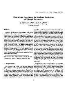
Figure 1: The rectangular computational domain mapped onto a
ux tube in a torus, with q0 = 2:4 and shear, s^ = 1:5. The ends of this ux tube are cut o� at poloidal angle ?� and �, and the sheared cross-sections of the ux tube in the poloidal plane are indicated.
!d , which using Eq. (4) is: i!d A � (cT=eB 2 )B � rB � rA = ?iky A(cT=eB0 R0) [cos � + s^(� ? �0 )sin �] ; (15) for ky 6= 0, and i!d A = ?ikx A(cT=eB0 R0 )sin �, for ky = 0. These coordinates are similar to those used in Ref. 18. Our �, , and z are analogous to ?q�0 , �0 , and �0 in Ref. 18, respectively, since they have chosen to measure the distance along the eld line with �0 , a \toroidal" angle, while we use �. A more signi cant di�erence between our representation and Ref. 18 is the treatment of periodicity and the boundary conditions along the eld line, though their more recent work19 has adopted a similar treatment to ours, described in Sec. III.
eik x+ik y A^k ;k (z; t); (11) x
y
x
y
with kx = j�=�x, ky = ?k�=�y, �x = q0� =B0 r0, and �y = r0��=q0. The rectangular computational box of \radial" width 2�x, and \poloidal" width 2�y, and extended along the eld line, �, is mapped onto a ux tube, as shown in Fig. 1, for example. While Eqs. (2,5,6) apply to general magnetic geometry, our simulations to date have used the traditional low- , large as- III. Periodicity and parallel boundary conditions pect ratio, concentric circular ux surface geometry. The speci c forms of these operators then take the usual ballooning The choice of parallel boundary conditions involves a numrepresentation forms (see Ref. 8 for more detail): ber of subtle, yet important issues. The main concept is that of a statistically-motivated periodicity, as described in Sec. II ; (12) b^ � rA = q 1R @A for the and � boundary conditions For moderately \balloon0 0 @� ing" turbulence we might expect parallel correlation lengths � � @A ? @� @A ; (13) �c � (1 ? 2)� (though it might be longer than this). The vE �rA = Bc2 B �r� �rA = Bc @� simulation box should have a length 2z0 = 2�N in the par@y @x 0 @x @y allel direction which is several times the parallel correlation length. In some cases a box length of 2� might be su�cient, and using the de nition of �0 in Eq. (22), kx = ?ky s^�0 , but a longer box may be necessary to ensure that one end r2 A = ?ky2 A[1 + s^2 (� ? �0 )2 ]: (14) of the box is su�ciently decorrelated from the other end to avoid arti cially constraining correlation e�ects, just as the Toroidal terms enter through the magnetic drift frequency, box must be at least a few correlation lengths wide in the ?
4
and � directions. For the cases simulated in Sec. VI, parallel box lengths of at least 4� were needed for good convergence. One must be careful about which other coordinates are held xed while applying parallel periodicity, just as one must be careful to impose radial periodicity in eld-line coordinates ( ; �; z) (i.e., impose periodicity in while holding � and z xed), as discussed in Sec. II. Though the ux-tube is rectangular in ( ; �) coordinates, it twists into a parallelogram in physical space as one follows the ux-tube along z. The
uctuations in the physical plane perpendicular to a magnetic eld line should be statistically identical at all places along that eld-line with the same poloidal angle (z = 0; 2�; 4�; : : :), irrespective of the twisting of the ux-tube which increases without bound as z ! 1. Because of this, we will assume that the uctuations are periodic in z while holding ( ; �) xed, rather than holding the eld-line coordinates ( ; �) xed. Speci cally, we impose:
box to the other. Note that �j must be an integer, so J = 2n0N�q must be an integer. This quantizes the range of q spanned by the ux tube, or the aspect ratio of the box, � =�� for q0 6= 0. One can treat shearless q0 = 0 cases as well, then �j = J = 0, and the radial box size 2� is no longer quantized. In the usual q0 6= 0 case, the radial position of the simulation box can be adjusted slightly so q0 is rational and Ck = 1. Eq. (19) thus expresses a modi ed periodicity condition on the mode amplitudes: the value of a coe�cient at one end of the box is speci ed by the value of another coe�cient with the same k but a di�erent j at the other end of a box. Since computer simulations cannot retain an in nite set of j's and k's, enough j and k modes are kept to resolve up to a desired value of k �i , above which the coe�cients A^j;k are assumed to vanish. Note that �j = 0 for k = 0 modes, so the periodicity condition for k = 0 modes simpli es to A^j;0(� + 2�N; t) = A^j;0(�; t). A( ; �(�; �); z(�)) �=N� = A( ; �(�; �); z(�)) �=?N� ; This completes the formal speci cation of the boundary conditions, but we go on to express it in terms of notation or often used in the ballooning transformation. It is common to A( ; �(� + 2�N; �); z(� + 2�N)) = A( ; �(�; �); z(�)): (16) introduce the \ballooning angle" �0 (j; k), such that the radial derivative of an individual (j; k) mode of Eq. (17), Physically, this is equivalent to considering two ( ; �) planes @ / i�(j=� ? kq0�=��); cutting through the ux tube, at z = � and at z = � + 2�N, (21) @ �;� and assuming that the turbulence is (statistically) identical in those two planes. To evaluate this periodicity constraint, rst substitute � = � ? q( )�, z = � into Eq. (7), and take �0 = 0 vanishes at � = �0 . Note that this de nition of �0 employs for simplicity. Since the ux tube is thin, we can approximate a derivative with respect to while holding � and � xed, q( ) � q0 + ( ? 0)q0 , where q0 � (@q=@ ) = 0 , so Eq. (7) not � and �. Clearly at � = �0 (j; k) the wavefronts of the j; k'th term in Eq. (7) are perpendicular to the surfaces. becomes: Eqs. (18,21) yield 1 X 1 X A= A^j;k (�; t) k�0 (j; k) = �j��q0 = nj��q : (22) j =?1 k=?1 0 �ei�( ? 0 )(j=� ?kq �=��)+ik��=��?ik�q0�=�� : (17) �0 is discrete with spacing ��0 = �=kn0 �q, which is dependent on k. Only the combination k�0 ever appears and the For convenience, we take the box width 2�� to be 1=n0 of limit k = 0 must be interpreted in terms of the discrete j sum. the full toroidal circumference, In particular, the turbulence can generate k = 0 (�0 = 1) modes corresponding to zonal ows which can be important �� = �=n0; (18) in the nonlinear dynamics, so the k = 0 modes must be allowed to evolve self-consistently. Similar care must be taken where n0 is a positive integer. Substituting this into Eq. (16) in the shearless limit q0 = 0, where �0 ! 1. Using the de ni8 yields: A^j +�j;k (� + 2�N; t)Ck = A^j;k (�; t); (19) tion of �0 in Eq. (22), we can express the shift �j in Eq. (20) as a shift in �0 instead: where the phase-factor Ck = exp(?i2�Nkq0n0 ), (23) ��0 = kn�j��q = 2�N: 0 �j = 2�Nkq � =�� = 2n0 kN�q; (20) 0 and 2�q = 2q0� is the change in q from one edge of the Using the de nition of �0 to denote A^j;k by a corre?
0
5
sponding A^�0 ;k , and absorbing a phase factor which is independent of the coordinates ( ; �; �) by using A�j;k = A^j;k exp[?ikn0 (q0�0 (j; k) + �0)]; the parallel periodicity condition of Eq.(19) can be written: A��0 +2�N;k (�; t) = A��0 ;k (� ? 2�N; t): (24) Using Eqs. (18) and (22) and q( ) � q0 + ( ? 0 )q0 (or going back to Eq. (7) and using q itself for the radial-like coordinate ), we can rewrite Eq. (17) as A( ; �; �; t) =
1 X
1 X
j =?1 k=?1
1
A�j;k (�; t)eikn0 [� ?q( )(�?�0 (j;k))];
2
3
4
5
6
A
(25) It should be emphasized that Eqs. (17) and (25) are merely the same equations in di�erent notation. Eq. (25) bears a strong resemblance to the standard ballooning representation. There are, however, important di�erences which are discussed in Sec. V. Eq. (25), when used with the periodicity relation in Eq. (24), is periodic in � with period 2�N. By setting N = 1, this can satisfy physical periodicity in �, achieving the same result as the \sum over p" in the standard ballooning representation. Thus, we are able to recover physical periodicity as does the quasiballooning approach.16 However, one should not necessarily use N = 1. Rather, one should use a large enough N so that the parallel box length 2z0 = 2�N is at least several times the parallel correlation length. This point may be confusing, since � is a physical variable, periodic over 2�. Of course, if we were simulating a full toroidal annulus with n0 = 1, we should choose N = 1. Indeed, Eq. (25) or (17) provides an expansion in a complete basis set if n0 = 1 and N = 1. However, we are not trying to simulate a full toroidal annulus, but a thin ux-tube whose width is only 1=n0 of the full toroidal circumference. Then Eq. (25) represents n0 identical copies of the simulation volume if one considers the full range of �, 0 ! 2�. Following the ux tube along the eld lines (at xed �) from � = 0 to � = 2� will not lead to the same physical location (unless q is an integer) but to one of the n0 ? 1 identical copies of itself. Forcing periodicity at this point is undesirable (unless the parallel correlation length is indeed signi cantly shorter than 2�) because it is a ction of simulating only 1=n0 of the toroidal direction with n0 identical copies. This is illustrated by Fig. 2, which shows a correlated volume with a parallel correlation length �c � 3�, and a perpendicular correlation length equal to half the simulation box width, �c = �� = �=6. If the simulation box has a parallel length of only 2�, this correlated volume would be forced to overlap with one of the n0 images of itself, causing ar-
Figure 2: Illustration on a ux surface of a possible correlated volume of the point 3 (enclosed by the solid line, with parallel correlation length �c � 3�), and a minimum simulation volume enclosed by the dashed line. The diagonal lines are parallel to the eld lines (here q = 2:4). In this case the simulation volume has a toroidal width of one sixth the total toroidal circumference, i.e. n0 in Eq. (18) is 6. If the potential is represented by Eq. (25) and � is made periodic in �, there are six identical copies of the correlated volume centered at the points 1-6. The correlated volume of point 5 (dotted line) partially overlaps the correlated volume of point 3, at the point marked A. This is unphysical and can be avoided in this case by making the system periodic over 4�, ?2� < � < 2�. The minimum simulation volume illustrated is for ?2� < � < 2�. ti cial interference e�ects. By extending the simulated ux tube to a length of 4�, we allow the whole region to evolve self-consistently. Of course, at an integer q ux surface, a simulation volume really does overlap itself within a distance � = 2� and experience these interference e�ects. More generally, a correlated volume will overlap itself when � increases by 2�N if q2�N modulo 2� is less than the perpendicular correlation length �c. This can be used to de ne a maximum parallel length �max which the ux-tube can be without physically overlapping itself. �max is also the maximum correlation length a correlated perturbation can have without \biting its tail" and experiencing coherent interference e�ects. �max is plotted vs. q( ) in Fig. 3. Note that if one simulates only 1=n0 of the toroidal direction, then a correlated perturbation is n0 6
of the plasma, there is no di�culty in extending the simulated
ux-tube to be 2-3 times longer than 2�, without having the
ux-tube physically run in to itself. Even for a simulation ux tube which spans a range of q values, for example 2�q � 1=2, at worst the ux tube might overlap itself brie y near an integer or half-integer q surface. As pointed out in Ref. 6, these low-order rational surfaces occupy a small fraction of a minor radius of a tokamak and so it is very infrequent that a correlated perturbation will \bite its tail." Furthermore, experimental evidence20 on tokamaks indicates that there are no unusual features near low-order rational surfaces, except when there are macroscopic MHD instabilities. In practice we nd that the ux-tube length 2�N doesn't need to be extremely large, and N = 2 may usually be suf cient. For the particular cases in Sec. VI, we nd that N = 1 simulations produce a �i which is about 30% low, while N = 2 ? 4 are virtually indistinguishable. However, there may be other cases where an even larger N is required. In each case, one should justify the value of N a posteriori, by verifying that the parallel correlation functions from the simulations indeed fall o� signi cantly in a distance 2�N, and/or by carrying out convergence studies with di�erent values of N, as in the perpendicular directions. We have also tested di�erent parallel boundary conditions. Instead of imposing parallel periodicity holding and � xed, Eq. (16), the perturbations could simply be zeroed, A( ; �; z = ��N) = 0, or we could impose periodicity in z at xed and �. While these two alternate boundary conditions should give the same result as our proposed method, Eq. (16), as the box length becomes very long, they do not converge as rapidly. We will concentrate on the case where periodicity in z is imposed at xed and �, so A( ; �; +�N) = A( ; �; ?�N), and each Aj;k mode in Eq. (7) is periodic with itself at z = ��N. In this case every eld line is e�ectively a rational eld line that connects to itself, since particles owing out one end of the box ow back in the other end on the same eld line. This is unlike a real sheared magnetic eld where most eld lines are irrational and never connect to themselves. This is particularly important for electron dynamics, since electrons move rapidly along the eld lines, and have time to sample a large fraction of the ux surface if q is irrational. When using the condition A( ; �; +�N) = A( ; �; ?�N) for the ions, we therefore distinguish between two ways of treating the electrons: treating q as rational everywhere for electrons, and treating q as irrational everywhere for electrons. If q is irrational, the eld line average h�i in the adiabatic electron response, ne = � ? h�i (see Appendix), is a ux surface average, and is zero unless ky = 0. If q is made rational everywhere, the eld line average h�i is a function of �, and is non-zero for ky 6= 0 modes, changing the quasineutrality constraint. This
Figure 3: Distance along the eld line, �max , at which a correlated
volume (with perpendicular width 2�� = �=25) overlaps itself, for varying q. a) For n0 = 1, �max is small only near low order q surfaces. b) For n0 = 6, the maximum correlation length is reduced, since the correlated volume can hit copies of itself. In this case, if the physical correlation length is longer than �max , the box must be extended and the periodicity condition relaxed.
times as likely to run into itself or one of its images. In this case we may need to extend the parallel length of the simulated ux-tube to avoid these arti cial correlations. For most 7
drastically changes the linear growth rates, and consequently, the turbulent heat ux. For the low shear cases in Sec. VI, the heat ux increases by a factor of 7. Even if we treat q as irrational for the adiabatic electron response, which is more realistic, using periodicity at xed ( ; �) for the ions yields heat di�usivities of (7:8; 4:5; 7;5)�2i vti =Ln for box lengths (2; 4; 6; 8)�, respectively, for the low shear cases in Sec. VI, while our approach converged to 5�2i vti=Ln at a box length of only 4�. The alternate boundary conditions converge more slowly because the ends of the box are wasted by not smoothly connecting the turbulence at each end. Speci cally, using A( ; �; +�N) = A( ; �; ?�N) causes discontinuities in the spatial gradient operators for a given ky and �0 mode across the ends of the box. For example, at � = �N, r2 A = ?ky2 Aj;k (�N)[1 + s^2 (�N ? �0 )2], while at � = ?�N, r2 A = ?ky2Aj;k (?�N)[1+ s^2 (?�N ? �0 )2], which is di�erent if �0 6= 0. This distorts the eddies and damps the turbulence near the ends of the box. If the ends are in the good curvature regions (lengths of 2�; 6�) the ux is high, and if the ends are in the bad curvature regions (4�; 8�) the ux is low. Our boundary condition Eq. (24) connects Aj;k (�N) to another mode with �0 shifted by 2�N to make the spatial operators continuous. ?
?
Figure 4: Boundary conditions in the parallel direction for particle
simulations. At � = 0, the simulation box is rectangular in � and . The twisted ends of the box at � = �N (solid) and � = ?�N (dashed) are shown. If a particle leaves the � = �N end of the box at �(1), it reenters the � = ?�N end of the box at �(2) , given by Eq. (26).
IV. Boundary conditions for particle simulations
copy of the original box, and is simply shifted by a multiple of 2�� back into the simulation domain. Expanding q( ), using Eqs. (18) and (19), and introducing an integer K to reproduce the modulo function, we nd: ��( ) = q Nn + K + J ( ? 0 ) : (27) 0 0 2�� 2� At the outer edge of the box, = 0 + � , the box has twisted by J=2 box lengths in the � direction, and by ?J=2 box lengths at the inner edge of the box, = 0 ? � . Thus J represents the integer number of box widths in � that the box has twisted from one end in z to the other end. This is illustrated for J = 2 in Fig. 4. In this gure, q0Nn0 is assumed to be an integer for simplicity, so the center of the box is at the same physical point at � = ��N. In general, the ends of the box will overlap with periodic copies of the original box. To summarize, if a particle leaves the box from ( 0 + � ; �; z) then it reenters at ( 0 ? � ; �; z); if it leaves from ( ; +��; z) then it reenters at ( ; ?��; z); and if it leaves from ( ; �; +�N) it reenters at ( ; � + ��; ?�N). All of the above boundary conditions are reversible, i.e., if a particle leaves at ( ? � ; �; z) it will reenter at ( + � ; �; z), etc.. More details on the implementation of boundary conditions
Particle simulations can also take advantage of an optimum
ux-tube simulation volume using the eld-line coordinates ( ; �; z) described in Sec. II. Field quantities such as the electrostatic potential can be represented by the Fourier series Eq. (7), with the parallel boundary conditions given by Eq. (19), or equivalently, Eq. (24). For the particles, we must specify the location where a particle will reenter the box after passing through an edge of the box. The particle's velocity should not be changed. In the perpendicular directions and �, standard periodicity is used. In the parallel direction, we apply Eq. (16). Using � = � ? q( )� and z = �, we see that if a particle exits the box at the position ( 1; �1; z = +�N), where �1 = �1 ? q( 1)�N, then it will reenter the opposite side of the box at ( 2 ; �2; z = ?�N), where 2 = 1, and �2 = �1 + q( 1)�N. Thus the particle will be shifted in � by the amount �� = �2 ? �1 = q( 1 )2�N modulo 2��
(26)
Where the modulo operation accounts for the fact that if this shift in � causes �2 to fall outside the range of the box, ?�� < � < ��, then the particle has fallen into a periodic 8
for particle simulations are given in Ref. 8.
in of the perturbations in ballooning space, and makes the ballooning transformation unique.23 If we set n0 = 1 in Eq. (25) and N = 1 in Eq. (19) we obtain an exactly equivalent representation to Eq. (29). To see this we note that the j in Eq. (25) and p and l in Eq. (29) are related by j = l ? 2pl0 and �j = 2l0 , and we set k = n. Thus the ?� < � < � range of the �� n;l modes with jlj < l0 correspond to the A�j;k modes with jj j < �j=2 (de ned only from ?� < � < � for N = 1). The A�j;k modes with jj j > �j=2 correspond to the ?� ? 2�p < � < � ? 2�p range of the �� n;l modes with p = (j ? l)=�j. The boundary condition Eq. (19) makes this series of A�j;k modes (for all j) identical to �� n;l (for jlj < l0 ) de ned on the extended domain ?1 < � < 1 (when n0 = N = 1). Using the boundary condition Eq. (19) and a nite � range simpli es the evaluation of the E � B nonlinearities compared to the usual ballooning representation. The simple form Eq. (6) is easy to evaluate using a pseudospectral method. A fully spectral method remains in k space at all times, so the nonlinear terms become convolutions in k space and require of order Nx2Ny2 Nz � N 5 operations. By using Fast Fourier Transforms (FFTs), the pseudospectral method reduces the operations to Nx Ny Nz (log2 Nx + log2 Ny ) � N 3 resulting in a very signi cant savings for large N. In the ballooning representation (i.e. using Eq. (29) to represent the perturbations) the nonlinear terms involve sums over p:24 X X X (vE � rA)n;l (�) = 2c n +n =n l p ;p
V. The Ballooning Transformation and its relation to ux tube simulation The linear theory of short perpendicular wavelength instabilities in tokamaks has been developed largely in terms of the so called \ballooning transformation."21 In this section we will discuss the relationship of the \ballooning transformation" to our ux tube simulation scheme. In ballooning theory a single eigenmode is represented as: �n ( ; �; �; t) =
1 X p=?1
e?i!t+in� ?inq( )(�?�0+2�p)
��^ n;�0 (� + 2�p; );
(28) where �0 = �0 ( ) and �^ n;�0 (�; ) depend on . The toroidal mode number n is any large integer. The variation in � and of the exponential is large whereas the variation of �0 and �^ is nite. In lowest order in an expansion in 1=nq one obtains a di�erential equation in � for �^ n;�0 (�; ). This equation is solved with �0 a parameter and with the boundary conditions �^ ! 0 as j�j ! 1, so the sum over p can converge. Periodicity in � is recovered by the p summation in Eq. (28). A lowest order approximation to the eigenvalue !n (�0 ; ) is obtained on each surface. In higher order the eigenvalue is quantized by solving radial di�erential equations. Much has been written about this higher order procedure to nd the radial behavior and we cannot do justice to the subtleties here.22 Let us consider instead a narrow radial annulus 0 ? � < < 0 +� . e?2�iq0 (n p +n p ) n0 n00q0 [2�(p00 ? p0 ) + �00 ? �000 ]� Let � be periodic in over 2� at constant � = � ? q( )� � �� n ;l (� + 2�p0 ) A�n ;l (� + 2�p00) and �; then we can represent the radial variation of � in a Fourier series in , with n�0 = l�=�q, i.e. the variation of 0 ) �� n ;l (� + 2�p00)� ; � (30) (� + 2�p ? A n ;l �0 ( ) and �^ n;�0 (�; ) are combined into a discrete series in �0 . Thus one could write for an arbitrary perturbation in this where l00 = l ? l0 +2�q(n0 p0 +n00 p00) and �0 (n; l) = l�=n�q. annulus: Again jl0j � jn0 j�q and jl00j � jn00j�q, and A� and �� are de ned on an in nitely extended � domain, without the bound�( ; �; �; t) = ary condition Eq. (19). This expression di�ers slightly from l0 1 1 X X X earlier literature since we are using a discrete representation ein� ?inq( )(�+2�p)+il�( ? 0 )=� in , and have implicitly used the inverse ballooning transn=?1 l=?l0 +1 p=?1 formation.23 If the mode width in � is less than �, the sums ��� n;l (� + 2�p; t); (29) over p appear to be a small e�ect, and are usually neglected in nonlinear calculations using the ballooning representation. where we have rescaled eilq0 �=q � �^ n;l = �� n;l . The p summa- This conclusion may be misleading. Noting that in Eq. (29) tion makes this expression manifestly periodic in �. Expand- kx = j�=�x = (l ? 2pl0 )�=�x and ky = ?n�=�y = ?nq0=r0, ing q( ), so exp[?inq2�p+il�( ? 0 )=� ] = exp[?inq02�p+ we see that in the standard ballooning representation, only a i�(l ? 2pn�q)( ? 0)=� ], it is clear that in this summa- wedge of �� n;l 's in (kx; ky ) space are evolved, ?n�q < l < n�q tion we need only take jlj � l0 = n�q since otherwise the (for n 6= 0), and the rest of k space is lled by the sum over p and l sums duplicate terms. This restricts the bandwidth p. For small n the evolved range of kx 's is small, so it may 0
0
0
00
00
0
0
00
00
0
0
00
00
0
?
9
00
0
0
00
take many terms in the p sum to reach moderate kx 's. The evolved wedge of kx modes corresponds to a wedge of �0 's from ?� < �0 < �. In our representation, since we evolve a rectangular grid in k space, the �0 range is not limited to j�0 j < �. The nonlinear interaction between a mode (kx ; ky ) within the p = 0 wedge and a mode outside the wedge could be strong, even if its linearly most unstable mode structure (of many eigenmodes in �) is centered a long distance down the eld line. For low ky and large kx one would have to include many p's to capture this interaction. In our nonlinear simulations, we do see modes outside the p = 0 wedge excited to signi cant amplitudes. While the form of the E � B nonlinearity in Eq. (6) can be e�ciently evaluated with FFTs, it is not obvious that Eq. (30) can be. However, since our representation is equivalent to the ballooning representation (if n0 = N = 1), it automatically includes the sums over p in the nonlinearity. Our representation should also be more convenient for analytic calculations, since the nonlinearity takes a simple form, and the choice of �0 's, or kx's, is well de ned. ?
VI. Simulation results We have implemented this coordinate system in nonlinear gyro uid simulations of toroidal ITG turbulence. The simulation results are presented here to describe practical computational issues and to test some of our assumptions. It is not meant to be a complete description of our gyro uid equations or our nonlinear results, which are discussed in Ref. 8. Therefore, we have relegated the actual equations to the Appendix. There are some subtleties involving the implementation of the boundary condition Eq. (19), because our equations involve jk j Landau damping terms (equivalent to a non-local integral operator in real space25 ). Two separate methods for implementing this boundary condition are described in detail in Ref. 8, which we refer to as the \equal-length extension" and \multiply-connected" methods. In practice, we have observed no signi cant di�erences between these methods in the nonlinear simulations done to date. These issues are ignorable for a particle or Vlasov simulation, since they do not require evaluation of kk and can directly use the boundary conditions in Sec. IV. To test the small-scale assumption, we present two simulations, one with perpendicular dimensions (Lx = 85�i , Ly = 100�i ), and one with double the box size (Lx = 170�i , Ly = 200�i). That these simulations give similar results indicates that the small ux tube may be capturing the essence of the turbulence. It is a necessary but not su�cient test, as discussed in Sec. VII. The physical parameters are taken from the Tokamak Fusion Test Reactor26 (TFTR) L-mode k
shot #41309: �i = 4, Ln =R = 0:4, s^ = 1:5, q = 2:4, Ti = Te , �i = :14cm, Ln = 103cm, and the computational box is centered at r0 = 53cm. The box sizes then correspond to n0 = 10 for the small box and n0 = 5 for the large box. Both simulations use 64 grid points along the eld line coordinate �. Using 128 grid points along � gives essentially the same results. For these runs, N = 2, so the physical � domain extends from ?2� to 2�. The equal length (�) extension method (for a total extended � domain from ?3� to 3�) was used to implement the parallel boundary condition. We use a spectral representation in x and y, with � 42 kx modes and � 15 ky modes for the small simulation and � 63 kx modes and � 21 ky modes for the large simulation, not counting additional modes added at high k for dealiasing. The modes are evenly spaced such that kymax �i � 1 and kxmin � kymin , making the computational domain roughly square in x and y. For N > 1, it is necessary to include more kx's to include unstable modes localized near � = �2�, �4�, etc., in the bad curvature regions (i.e. modes with �0 's near �2�, �4�, etc.). The modes tend to be localized along the eld line near �0 , so ideally one would like to include enough kx's to cover the range ?�N < �0 < �N for all ky 's. This is very expensive at high ky , where the spacing in �0 gets small, since �0 = ?kx =^sky . We arrange our modes in k space so that the �0 's cover the � domain for low ky 's, but not high ky 's. This implies kxmax � kymax for N > 1 and s^ � 1. Since most of the energy is at ky �i < 1=2, the missing �0 's at high ky have very little e�ect. Fig. 5 shows contours of electrostatic potential in the (x,y) plane at � = 0 (the outer midplane of the torus), for both runs at saturation. (The uctuations on the inner midplane have roughly 1/2 the amplitude, which would be an interesting feature to look for in experiments.) It is apparent that although the box was doubled, the dominant scale didn't change. This is also evident from the spectra in Fig. 6, also at � = 0, where j�j2(kx ) = Pk �k ;k ��k ;k , j�j2(ky ) = Pk �k ;k ��k ;k , and the low resolution spectra are reduced by a factor of two to account for mode density. Although the resolution has increased, the shape and the location of the peak in the spectrum is roughly the same. These spectra are similar to BES measurements on TFTR.1 The large ky = 0 component is evidence of sheared zonal E � B ows,7 which are primarily in the poloidal direction. Though there are some small di�erences in the spectra, the two runs agree within statistical uctuations on global quantities such as the volume averaged RMS uctuation levels and transport levels: e�=Ti = 15�i =Ln ' 0:020 and �i = 7:4�2i vti=Ln , averaged from tvti =Ln = 150 ? 300. The statistical uctuations in �i at saturation are about 10% for both runs. This level of ion heat transport is near the experimentally measured �i = 8:8�2i vti =Ln, but these simulations ignore impurities and
10
y
x
y
x
y
x
x
y
x
y
Figure 5: Contours of potential for a) small run, and b) large run. Doubling the perpendicular simulation domain did not change the dominant scale of the uctuations. beams (usually a stabilizing e�ect), trapped electrons (destabilizing), and use our four moment model which gives lower transport than our more accurate six moment model. Nevertheless, this level of agreement is encouraging, and suggests that toroidal ITG turbulence is responsible for anomalous ion heat transport in tokamaks. The transport from these toroidal simulations is about a factor of 25 larger than sheared slab simulations for the same parameters, demonstrating the 11
Figure 6: Potential spectra for both runs. importance of toroidicity. Our toroidal simulations can be run in the sheared slab limit by taking Ln =R ! 0 and q=^s ! 0 so that Ln=Ls = Ln s^=qR remains nite. We should point out that our preliminary results, Fig. 2a of Ref. 7, were high by a factor of 16/3 due to a numerical error in calculating �i . The
remaining change is due to increased resolution. We have also performed tests varying the box length in the parallel direction. For these tests we have used the \multiply connected" method to implement the parallel boundary conditions, for greatest accuracy, as described earlier in this section. Fig. 7a shows the time evolution of the volume averaged �i for two runs with box length N = 1 and 2, i.e. �� = 2� and 4�, with n0 = 10, and other parameters as above. Fig. 7b shows the correlation function along the eld line, y; �)�(x; y; � = 0)i ; (31) C(�; 0) = h�(x;h�(x; y; � = 0)2i for the two runs. The averaging h i is over x, y, and time once the simulation has reached a quasi-steady state. If this correlation function were not averaged in x and y (only taken along the eld line passing through x = y = 0), it would return to one at � = �2� for the N = 1 run, because of periodicity. The Fourier transform of C(�; 0) is the k spectrum. As discussed in Sec. III, since n0 > 1, using a box with ?� < � < �, (N = 1), can arti cially constrain the parallel correlation length. There are signi cant correlations at � � � for these parameters, indicating that this is the case, and that the box should be extended. These additional correlations in the 2� box are in some way constraining the nonlinear dynamics and reducing the ux. It is easier to test the scaling with box length at low shear, since the turbulence at �2�, �4�, etc., is not at such high kx , because kx = ?ky s^�0 . This allows resolution of the turbulence along the entire box length with fewer kx modes than at high shear. Also, at low shear the linear mode structure is broader in �, leading to slightly broader parallel correlation functions. Fig. 8a shows the time evolution of �i in four runs with box lengths N = 1; 2; 3; 4 or �� = 2�; 4�; 6�; 8�. The physical parameters are the same as above, except s^ = 0:1 and q = 1:2, and the perpendicular box size is Lx = 160�i , Ly = 100�i. Again, the �� = 2� box gives slightly lower ux, while the longer boxes all give the same ux, so the minimum box length is �� = 4�. The correlation functions of electron density for these runs are shown in Fig. 8b, and are noticeably broader than in the higher shear cases. Using ne in the correlation functions removes the k = 0 component present in the � correlation functions in Fig. 7b, since ne = � ? h�i (see Appendix). For these low shear runs, the poloidal spectrum peaks at ky �i = 0:35, so the perpendicular correlation length is smaller than in the high shear cases. This may contribute to the slightly smaller change in ux in going from �� = 2� to �� = 4�, even though the parallel correlation functions are broader. These low shear runs are better resolved than the high shear runs in Fig. 7, so we expect that a 30% change in ux when the arti cial correlations are rek
k
Figure 7: a) Evolution of �i for two runs with varying box length and s^ = 1:5, q = 2:4 b) Correlation functions along the eld line for the same two runs. moved by using a longer box is typical for ITG turbulence, where �c � 2�. We have also run with s^ = 0:1 and q = 2:4, where �i = 7:5�2i vti=Ln for �� = 4� and �i = 6:5�2i vti=Ln
12
VII. Discussion and Conclusions
Figure 8: a) Evolution of �i for four runs with varying box length and s^ = 0:1, q = 1:2. b) Correlation functions along the eld line for �� = 2� and 4�. for �� = 2�. For s^ = 0:25 and q = 1:2, both �� = 2� and �� = 4� give �i = 5�2i vti =Ln, any change is within the statistical uctuations.
To summarize, we are simulating a rectangular domain in (x; y; z), and using the transformation Eq. (10), this domain becomes a long, thin, twisting ux tube in a torus. The di�erential operators take the particularly useful forms Eq. (2-6), applicable to general magnetic geometry; only the metric coe�cients r�, r , and rz need to be speci ed. The boundary condition Eq. (19) can make the perturbations periodic in �, if N = 1, which makes this representation equivalent to the ballooning representation for a coarse grid in n, with spacing n0. However, when n0 > 1, the box must be extended in � to avoid non-physical correlations if the parallel correlation length is longer than 2�qR, i.e. �c > 2�. The fundamental assumptions are that the correlation lengths (both parallel and perpendicular) are smaller than the box size, that the equilibrium gradients vary slowly across the small perpendicular extent of the box, and that the turbulence is local, i.e. driven only by the equilibrium gradients within the box. The assumptions implicit in simulating a thin ux-tube subdomain should always be checked a posteriori by verifying that the simulation box is indeed at least a few correlation lengths long in each direction, so that the box is large enough for the type of turbulence under consideration. One should also verify that the results are independent of the size of the simulated ux tube (and independent of the particular choice of boundary conditions), as the ux tube is made larger than the correlation lengths. This paper has demonstrated that both conditions are met, at least for the particular cases considered in Sec. VI. Our gyro uid equations have been scaled to the gyroradius �i , and the limit �i =Ln ! 0 taken, using the usual small-scale turbulence ordering assumptions, thus the box-size independence implies gyro-Bohm scaling with magnetic eld, B, at least for su�ciently small �� = �i =Ln. While the turbulent heat conduction from our simulations is of the right order of magnitude to explain experimental results from the core region of many tokamaks, the experiments indicate a Bohm-scaling27,28 with B, not gyro-Bohm. Several possibilities for this discrepancy exist. One is that the experimental �� , while small (� 10?3 ? 10?2 ), may be large enough that the radial variation of equilibrium gradients, i.e. !� ( ), �i( ), etc., or equilibrium ows, may be a�ecting the turbulence. For very small �� there is a scale separation between the turbulence, with scales of order �i , and the equilibrium, with scale Ln , but if �� is not small enough, the turbulence may begin to feel radial variations in the equilibrium. It is interesting to note that the BES measured1 correlation length �c � 2 cm is of order the geometric mean between �i � 0:15 cm and the minor radius a � 90 cm. Another possible explanation is that the instabilities driving the turbulence may be near marginal stability, which can mask gyro-Bohm scal13
ing trends and, in some limits, tie the core transport scaling to edge parameters.29{31 A very sensitive dependence on some parameters which vary slightly while scaling �� could also partially mask a gyro-Bohm scaling. Another explanation might involve nonlocal turbulence, where uctuations radially propagate a signi cant distance from where they were generated by an instability, an e�ect which is currently under debate.32,33 Numerical studies of some of these e�ects do not necessarily require simulating the whole tokamak. Rather, one could consider a somewhat thicker ux-tube than usual, and include the radial variations of !� ( ), �i ( ), and other plasma parameters over the simulated region. Even if simulating the full torus radially, eld-line coordinates are useful to allow a coarser grid in the parallel direction, and a coarser grid in the toroidal mode number n. When the equilibrium pro les are assumed to be constant, so Ln , LT , etc. do not vary radially (as assumed in our simulations), the linear eigenmodes are unbounded radially. In ballooning terminology, the solutions of the zeroth order eigenmode equation in 1=nq are independent of . In a real tokamak, however, the radial pro le variation determines the radial extent of the linear modes, and this radial structure is determined from a higher order equation in 1=nq. Recently, there has been renewed interest in the solution for this radial envelope, and the modi cations to the zeroth order eigenfrequencies.22 For longer wavelength global modes, the linear radial mode structure is also determined by the radial variation of equilibrium gradients.34 An alternative way to include these e�ects is to still use Eq. (7) to represent the perturbations. The dependence of the equilibrium will then linearly couple di�erent j modes in Eq. (7), which are uncoupled when the pro les have constant gradients. Then the superposition of di�erent j (i.e. kx) modes will determine the radial envelope of the true linear mode. However, since the nonlinear E � B coupling of the various A^j;k modes is usually much stronger than this linear coupling, it is likely that the precise radial linear mode shape is subdominant, and that the radial scale length of the turbulence is set by nonlinear processes, as suggested in Refs. 6 and 35. Comparing the order of magnitude of these e�ects in, for example, the density equation, we have: 1 2 e� n1 n0 vE � rn1 � �i vti k Ti n0 ; � � �� 1 v � rn (x) � �i vti ky e� 1 + O x ; 0 n0 E Ln Ti L� Where L� is the scale length for the radial variation in Ln , and is typically of order Ln . The nonlinear term is of the same order as the x independent linear term (i.e. the !� ( 0) term) in the standard gyrokinetic ordering, where n1 =n0 � �i =Ln and k �i � 1. As the linear mode widths get broader radi?
?
ally (in x), the x=L� terms become more important. While the linear modes are broad, the typical turbulent eddy size is not much larger than �x � 10�i , so it would seem that the x-dependent term (/ @!� =@ ) can safely be ignored, as long as �x � L� . The e�ects of radial variations in the equilibrium may start becoming important if �� = �i =L� is large enough, and could lead to a transition from gryo-Bohm to Bohm behavior.36 From the above arguments, it would seem that experiments should have small enough �� to be in the gyro-Bohm regime, though TFTR seems to be in the Bohm regime.27,28 Equilibrium sheared zonal ows (ky = 0; kz = 0; kx 6= 0
ows which cause ux surfaces to rotate) can be included in our representation in several ways (one of which is presented in Ref. 19), though we have not yet implemented them in our simulations. Such sheared ows can be important, particularly near the plasma edge where they appear to be responsible for the H-mode transition.37 Though we are presently neglecting equilibrium-scale zonal ows, we do include the higher kr components of the zonal ows which are generated by the turbulence itself. For typical tokamak parameters, our reduced simulation volume can represent large computational savings. We compare rough scalings with some other methods; the results are only order of magnitude estimates. Perhaps the most straightforward way to simulate a tokamak is with the \m; n; r" representation: X (32) �( ; �; �) = ein� ?im� �^ m;n ( ): m;n
Since we are interested in simulating ne-scale turbulence, we need to resolve perpendicular scales of order �i . If we are simulating a full torus, the range of m's must be m 2 (0; �1; : : :; �a=�i ). To resolve the long parallel structure, the range of n's must be n 2 (0; �1; : : :; �a=q�i ), where q is a representative value, around 2. The radial grid for �^ m;n ( ) must resolve �i and span the minor radius, so r = l�r , where �r � �i and l 2 (0; 1; : : :; a=�i). This gives� the total number �3 of grid points, for a � 103�i , Nm;n;r � q1 �a � 109. This is the same as expected from a computational grid in the physical r; �; � space, where the � grid can be 1=q coarser than the r or � directions. By simulating a thin toroidal annulus in r, but still going all the way around in � and �, the number of radial grid points is reduced by �r=a, which for our simulations is typically 1/10. Further, aligning the grid points with the eld lines reduces the necessary resolution in this direction. We have found that 64 grid points along the eld line is adequate, so the number of grid points for a thin annulus with a eld-aligned coordinate
14
i
�2
�
is: Nannulus � 64 �a �ar � 107. The next level of reduction is to also exploit the small perpendicular correlation length in the poloidal direction, which brings us to our twisting ux tube: N ux tube � � �2 a 64 � �ar �ay � 106; so for the simulation in Fig. 5a, including modes for dealiasing, we used: N � 64 � 128 � 48 � 4 � 105. This is roughly 103 times fewer grid points than a full torus simulation with the same resolution. Kotschenreuther and Wong15 have proposed using the representation: X �(r; �; �) = eil(m0 �?n0 � ) eij� �^ j;l (r ? r0); (33) i
i
j;l
which has many similarities to our representation. It is periodic in � with period 2�=n0 and in � over 2�, and is therefore simulating a wedge of a toroidal annulus when the r domain is small. Thus Eq. (33) is as e�cient as the one described in this paper, however, if �c > 2� false correlations along the parallel direction will be introduced, as discussed in Sec. III. It is not obvious how to remedy this problem with Eq. (33), but with our approach one simply uses a longer box, i.e. N > 1. The \quasiballooning" approach of Dimits16 shares similar computational advantages to our method. Indeed, the quasiballooning (almost- eld-line coordinates) method has many similarities to the eld-line coordinates approach of Roberts and Taylor,5 and Cowley, et al.,6 upon which our paper is based, though the quasiballooning method emphasizes the perspective of a real-space radial grid while we use discrete Fourier transforms for the radial direction which illustrate its relation to the usual ballooning transformation. We have shown that physical periodicity in � can be also be implemented with our approach, but that there are cases where one should forgo physical periodicity in favor of a longer box (i.e., N > 1) to avoid false parallel correlations. As described in Sec. III, simulating only 1=n0 of the toroidal direction is often justi ed by the short perpendicular correlation lengths of the turbulence, but that makes a perturbation extended along a eld-line n0 times as likely to \bite its tail," which should be compensated for by making the box longer than a parallel correlation length. In principle, N = 1 simulations should eventually converge as the box is made large enough in the perpendicular directions (so that n0 ! 1), but from the runs we have done it appears that faster convergence is obtained by allowing the box to be longer than a parallel correlation length as well, thus consistently following the principle that the simulation domain should be longer than the correlation lengths in all three directions.
Acknowledgements
The authors thank R. E. Waltz and G. D. Kerbel for useful discussions. Our toroidal nonlinear gyro uid code grew out of the earlier slab gyro uid code developed by W. Dorland,10,38 who provided helpful computational advice and physics discussions. M.A.B. also thanks Q. P. Liu, D. P. Coster, and M. Artun for further useful discussions and computational advice. M.A.B. and G.W.H. thank the TFTR project for supporting this work, and the National Energy Research Supercomputer Center for computing resources. This work supported in part by the High Performance Computing and Communications Initiative (HPCCI) Grand Challenge Numerical Tokamak Project, by USDoE contract No. DE-AC02-76-CH03073, contract No. DE-FG03-93ER54224, and by a National Science Foundation Graduate Fellowship.
Appendix. Toroidal gyro uid equations The equations used in the simulations are a subset of those derived in detail in Ref. 8, and are brie y summarized here. In these simulations, we evolve four moments of the gyrokinetic equation, the perturbed guiding center density, parallel
ow, parallel temperature, and perpendicular temperature, with closure approximations to model the e�ects of parallel resonances,25 toroidal resonances,39,40 and FLR.41 Here we ignore collisions and particle trapping (i.e. b^ � rB = 0), although we have developed models of these e�ects, and have extended this model to up to six moments.7 Using the normalizations in Ref. 41, the dynamical equations are: � � dn + b^ � ru + �1 + �i r^ 2 � @ + 1 r^ 2 v � rT = dt 2 @y 2 ? i!d (T + T + 2n + 2 ) ; du + b^ � r(T + n + ) = ?2i! � u ? 2j! j� u ; d 5i d 5r dt dT + 2b^ � ru + p2jk j� T + � @ = i @y dt ? 2i!d [(3 + �1i)T + �2iT + n + ] ? 2�1r j!djT �? 2�2r j!d jT �; dT + p2jk j� T + 1 r^ 2 dt 2 � � 2 1 + 2 r^ 2 + �i(1 + r^ ) @ @y � � 2 1 + 2 r^ 2 v � rn + (r^ v ) � rT � � n 1 3 2 ^ = ?2i!d �3iT + (2 + �4i)T + 2 + 2 (1 + 2 r ) ? 2�3r j!djT ? 2�4r j!d jT : k
?
k
?
k
k
k
k
k
k
k
k
k
k
?
k
?
?
k
?
?
?
?
?
?
?
?
k
k
15
?
?
?
?
?
The total time derivative includes the E � B nonlinearities, d=dt = @=@t + v � r. The gyroaveraged potential and E � B drift are = ?10=2� and v = b^ � r , respectively. The toroidal drift terms have been written using i!d � (cT=eB 2 )B � rB � r. The closure coe�cients for this set of moments are chosen to provide an accurate approximation to the linear kinetic response. The parallel closure coe�cients are � = 2=p� p and � = 1= �. The toroidal closure coe�cients have both dissipative and reactive pieces, and written in the form � = (�r ; �i) = �r + i�i j!dj=!d , they are �1 = (1:93; ?:39), �2 = (:24; 1:29), �3 = (?1:40; :47), �4 = (?:14; ?1:75), and �5 = (:76; ?:98). We assume adiabatic electron response, ne = �R (� ? h�i), where � = Ti =Te , and h�i( ) = R ( d�dzJ jr j�)= ( d�dzJ jr j) is a ux surface average. In circular concentric geometry, this becomes h�i = R (4�y z0 )?1 dy dz(R=R0)�(x; y; z), and is only nonzero for the ky = 0 components. This form of the adiabatic electron response prevents radial electron ow which would short out the electric eld responsible for the nonlinearly generated sheared poloidal ows which are essential for saturation.7 The gyrokinetic quasineutrality constraint is ne = n� i + (?0 ? 1)�, where n� i is the ion density in real space, which is related to the ion guiding center density and perpendicular temperature by the FLR closure relation in Ref. 41, yielding: k
?
?10=2 �N(b) n + 1 r^ 2 T � + (? ? 1)�: � (� ? h�i) = D(b) 0 2 ?
?
The functions N(b), D(b), where b = k2 �2i , and the operators r^ and r^ model FLR e�ects, and explicit forms are given in Ref. 41. Since this equation involves both � and h�i, we use the following procedure to determine �, given n and T . In general, the coe�cients in this equation can be functions of the eld line coordinate, so writing � = h�i + ��, and solving for �� gives: �� = [�ni + (?0 ? 1)h�i]=(� + 1 ? ?0 ). Now ux surface averaging ��, since h��i = 0, and solving for h�i gives: h�i = h � + 1n�i? ? i=h � (1+ ?1 ??0?) i: 0 0 Now that h�i is determined, we use this expression in the quasineutrality constraint to obtain �. ?
?
?
?
References 1
R. J. Fonck, G. Cosby, R. D. Durst, S. F. Paul, N. Bretz, S. Scott, E. Synakowski, and G. Taylor, Phys. Rev. Lett. 70, 3736 (1993).
E. Mazzucato and R. Nazikian, Phys. Rev. Lett. 71, 1840 (1993). S. Zweben and S. S. Medley, Phys. Fluids B 1, 2058 (1989). 4 S. E. Parker, J. C. Cummings, W. W. Lee, and H. E. Mynick, in Proceedings of the Joint Varenna-Lausanne International Workshop on Theory of Fusion Plasmas, (Societa Italiana di Fisica, Bologna, 1994). 5 K. V. Roberts and J. B. Taylor, Phys. Fluids 8, 315 (1965). 6 S. C. Cowley, R. M. Kulsrud, and R. Sudan, Phys. Fluids B 3, 2767 (1991). 7 G. W. Hammett, M. A. Beer, W. Dorland, S. C. Cowley, and S. A. Smith, Plasma Phys. Controlled Fusion 35, 973 (1993). 8 M. A. Beer, Ph.D. Thesis, Princeton University (1994). 9 M. D. Kruskal and R. M. Kulsrud, Phys. Fluids 1, 265 (1958). 10 W. Dorland, G. W. Hammett, T. S. Hahm, and M. A. Beer, in U. S.-Japan Workshop on Ion Temperature Gradient Driven Turbulent Transport, edited by W. Horton, M. Wakatani, and A. Wootton, (American Institute of Physics, New York, 1993), p. 344. 11 B. Cohen, T. J. Williams, A. M. Dimits, and J. A. Byers, Phys. Fluids B 5, 2967 (1993). 12 A. Hasegawa and M. Wakatani, Phys. Rev. Lett. 59, 1581 (1987). 13 B. A. Carreras, V. E. Lynch, and L. Garcia, Phys. Fluids B 3, 1438 (1991). 14 P. H. Diamond and Y. B. Kim, Phys. Fluids B 3, 1626 (1991). 15 M. Kotschenreuther and H. V. Wong, private communication (1991). 16 A. M. Dimits, Phys. Rev. E 48, 4070 (1993). 17 J. M. Greene and J. L. Johnson, Phys. Fluids 5, 510 (1962). 18 R. E. Waltz and A. H. Boozer, Phys. Fluids B 5, 2201 (1993). 19 R. E. Waltz, G. D. Kerbel, and J. Milovich, Phys. Plasmas 1, 2229 (1994). 20 M. C. Zarnstor�, S. Batha, A. Janos, F. L. Levinton, and the TFTR Group, in Local Transport Studies in Fusion Plasmas, edited by J. D. Callen, G. Gorini, and E. Sindoni, (Societa Italiana di Fisica, Bologna, 1993), p. 257. 21 J. W. Connor, R. J. Hastie, and J. B. Taylor, Proc. R. Soc. London A 365, 1 (1979); A. H. Glasser, in Proceedings of the Finite Beta Theory Workshop, Varenna, 1977, edited by B. Coppi and W. Sadowski (U. S. Department of Energy, CONF-7709167, 1977), p. 55; Y. C. Lee and J. W. Van Dam, ibid., p. 93. 22 J. W. Connor, J. B. Taylor, and H. R. Wilson, Phys. Rev. Lett. 70, 1803 (1993); J. B. Taylor, J. W. Connor, and H. R. Wilson, Plasma Phys. Controlled Fusion 35, 1063 (1993); N. Mattor, Phys. Plasmas 1, 245 (1994). 23 R. D. Hazeltine and W. A. Newcomb, Phys. Fluids B 2, 7 (1990). 24 E. A. Frieman and Liu Chen, Phys. Fluids 25, 502 (1982). 25 G. W. Hammett and F. W. Perkins, Phys. Rev. Lett. 64, 3019 (1990).
16
2
3
R. J. Hawryluk, D. Mueller, J. Hosea, C. W. Barnes, M. A. Beer, M. G. Bell, R. Bell, H. Biglari, M. Bitter, R. Boivin, N. L. Bretz, R. V. Budny, C. E. Bush, L. Chen, C. Cheng, S. Cowley, D. Darrow, P. C. Efthimion, R. J. Fonck, E. Frederickson, H. P. Furth, G. Greene, B. Grek, L. R. Grisham, G. W. Hammett, W. W. Heidbrink, K. W. Hill, D. Ho�man, R. Hulse, H. Hsuan, A. Janos, D. L. Jassby, F. C. Jobes, D. W. Johnson, L. C. Johnson, R. Kamperschroer, J. Kesner, C. Phillips, S. J. Kilpatrick, H. Kugel, P. H. LaMarche, B. LeBlanc, D. M. Manos, D. K. Mans eld, E. Marmar, E. Mazzucato, M. P. McCarthy, J. Machuzak, M. Mauel, D. C. McCune, K. McGuire, S. S. Medley, D. R. Mikkelsen, D. Monticello, Y. Nagayama, G. Navratil, R. Nazikian, D. K. Owens, H. Park, W. Park, S. F. Paul, F. W. Perkins, S. Pitcher, D. Rasmussen, M. H. Redi, G. Rewoldt, D. Roberts, A. L. Roquemore, S. Sabbagh, G. Schilling, J. Schivell, G. L. Schmidt, S. D. Scott, J. Snipes, J. Stevens, W. Stodiek, B. C. Stratton, J. Strachan, E. Synakowski, W. M. Tang, G. Taylor, J. Terry, J. R. Timberlake, H. H. Towner, M. Ulrickson, S. von Goeler, R. Wieland, J. Wilson, K. L. Wong, P Woskov, M. Yamada, K. M. Young, M. C. Zarnstor�, and S. J. Zweben, Fusion Technol. 21, 1324 (1992). 27 S. D. Scott, C. W. Barnes, D. M. Mikkelsen, F. W. Perkins, M. G. Bell, R. E. Bell, C. E. Bush, D. E. Ernst, E. D. Fredrickson, B. Grek, K. W. Hill, A. C. Janos, F. C. Jobes, D. W. Johnson, D. K. Mans eld, D. K. Owens, H. Park, S. F. Paul, A. T. Ramsey, J. Schivell, B. C. Stratton, E. J. Synakowski, W. M. Tang, and M. C. Zarnstor�, in Plasma Physics and Controlled Nuclear Fusion Research 1992 (International Atomic Energy Agency, Vienna, 1993), Vol. 3, p. 427. 28 F. W. Perkins, C. W. Barnes, D. W. Johnson, S. D. Scott, M. C. Zarnstor�, M. G. Bell, R. E. Bell, C. E. Bush, B. Grek, K. W. Hill, D. K. Mans eld, H. Park, A. T. Ramsey, J. Schivell, B. C. Stratton, and E. Synakowski, Phys. Fluids B 5, 477 (1993). 29 P. W. Terry, J.-N. Leboeuf, P. H. Diamond, D. R. Thayer, J. E. Sedlak, and G. S. Lee, Phys. Fluids 31, 2920 (1988). 30 H. Biglari, P. H. Diamond, and M. N. Rosenbluth, Phys. Fluids B 1, 109 (1989). 31 M. Kotschenreuther, H. L. Berk, M. Lebrun, J. Q. Dong, W. Horton, J.-Y. Kim, Y. Kishimoto, D. W. Ross, T. Tajima, P. M. Valanju, H. V. Wong, W. Miner, D. C. Barnes, J. U. Brackbill, K. M. Ling, R. A. Nebel, W. D. Nystrom, J. A. Byers, B. I. Cohen, A. M. Dimits, L. L. Lodestro, N. Mattor, G. R. Smith, T. J. Williams, G. D. Kerbel, J. M. Dawson, R. D. Sydora, B. A. Carreras, N. Dominguez, C. L. Hedrick, J.-N. Leboeuf, H. Naitou, and T. Kamimura, in Plasma Physics and Controlled Nuclear Fusion Research 1992 (International Atomic Energy Agency, Vienna, 1993), Vol. 2, p. 11. 32 X. Garbet, L. Laurent, J. P. Roubin, A. Samain, in Plasma Physics and Controlled Nuclear Fusion Research 1992 (International Atomic Energy Agency, Vienna, 1993), Vol. 2, p. 213. 33 N. Mattor and P. H. Diamond, Phys. Rev. Lett. 72, 486 (1994). 34 W. M. Tang and G. Rewoldt, Phys. Fluids B 5, 2451 (1993). 35 N. Mattor, Phys. Fluids B 3, 1913 (1991).
26
G. W. Hammett, M. A. Beer, J. C. Cummings, W. Dorland, W. W. Lee, H. E. Mynick, S. E. Parker, R. A. Santoro, M. Artun, H. P. Furth, T. S. Hahm, G. Rewoldt, W. M. Tang, R. E. Waltz, G. D. Kerbel, and J. Milovich, in Plasma Physics and Controlled Nuclear Fusion Research 1994, paper IAEA-CN-60/D-2-II-1, (to be published by the International Atomic Energy Agency, Vienna, 1995). 37 H. Biglari, P. H. Diamond, and P. W. Terry, Phys. Fluids B 2, 1 (1990). 38 W. Dorland, Ph.D. Thesis, Princeton University (1993). 39 R. E. Waltz, R. R. Dominguez, and G. W. Hammett, Phys. Fluids B 4, 3138 (1992). 40 M. A. Beer, G. W. Hammett, W. Dorland, and S. C. Cowley, Bull. Am. Phys. Soc. 37, 1478 (1992). 41 W. Dorland and G. W. Hammett, Phys. Fluids B 5, 812 (1993).
36
17