FIFO Networking: Punctual Event-Triggered Communication Viktor Leijon∗ Department of Computer Science and Electrical Engineering, Lule˚a University of Technology, Lule˚a, Sweden. E-mail:
[email protected] Abstract It is desirable to be able to combine ease of implementation of a network with the ability to analyze the properties of the network. In order to address this we present a MAC protocol where the network acts as a FIFO, and examine the resulting properties of the network using both a theoretical study of the waiting times and a simulation experiment. It turns out that this type of protocol would allows us to achieve real-time guarantees for an eventtriggered system, as well as controlled jitter for message delivery. Further, temporal composability, and how to design a system using FIFO networking, is discussed.
1. Introduction Time deterministic behavior is often considered to be one of the main benefits of time-triggered busses such as TTCAN [12] and TTP/C [18]. Conversely this is seen as a weakness [2] for event-triggered buses such as the Controller Area Network (CAN) [8]. On the other hand, the event-triggered paradigm is perceived as more natural than time-triggered, in the words of Almeida et al. [2]: ”event-triggered communication does seem more ergonomic and even more resource efficient”. In this article we will bridge the perceived gap in predictability between the time-triggered and event-triggered paradigms, and to do this in a way that is as simple and transparent as possible. The key idea is modeling the network as a first in-first out (FIFO) channel, a queue where messages are delivered in the same order that they are queued. Compared to a purely priority based systems we gain composability, simple analysis even for non-periodic tasks, and improved jitter control. We also remove the need to provide priorities, and eliminate the risk of starvation. In an earlier paper [13] we outlined the general principles of FIFO networking and discussed a prototype implementation. This paper expands on it by providing a queue theoretical analysis as well as in depth simulations and a ∗ This
work was supported by the EU FP6 project SOCRADES.
978-1-4244-2728-4/09/$25.00 ©2009 IEEE
discussion of possible extensions of the paradigm. In summary our contributions are: • First we present and discuss what we perceive as the consensus about which timing properties are central for a hard real-time networked system, Section 2.1. • We suggest using an event-triggered network and viewing the bus as a FIFO with a limited number of slots. We show a way to accomplish this without putting control over the FIFO in any single node. This model could be viewed as a token based network with a virtual token. • We show how it gives us predictable maximum delay for our messages (Section 2). • We show how this model could be implemented on a standard CAN bus (Section 3) and describe how we are able to achieve predictable delay as well as jitter control (Section 3.2). • We define the conditions for achieving temporal composition of services (Section 2.5), and we contrast this what is achieved in a time-triggered network. • We compare our model to other networking paradigms through a simulation study, Section 4.
2. The network as a FIFO 2.1. Central timing properties. There are many different approaches to deciding who gets to use the network at any given time. In a timetriggered network it is decided a priori, and the static schedule decides when a node is allowed to transmit. In an event-triggered system some other method is needed; in the Ethernet protocol chance decides who gets to transmit, and in a static priority based system a priority is used to arbitrate between concurrent senders. Many systems also function as hybrids of these methods. Ideally, statements about different paradigms should be as specific and objective as possible, and to this end we try to state some criteria which will help us determine if a communication paradigm is suitable for hard real time
Modeling the network as a FIFO avoids both starvation and the need to decide priorities for communication streams, even for a system where composition is desired. In situations where the system is expected to be overloaded, prioritization is clearly needed, the FIFO approach can be extended with priorities as outlined in Section 3.3.
Figure 1. A FIFO for messages systems or not. There appears to be some consensus [1, 2, 9] about what is important, which we try to express in the following definition: Definition 1 (Central Timing Properties) The following three properties are those that a communications system must have to be suitable for use in hard real-time systems. Latency. It must be possible to give a strict upper bound on the message delivery time for real-time communications. Jitter. The maximum and minimum delivery times should be known, and preferably be as close together as possible. Composability. Timing properties of correctly constructed subsystems will not be destroyed by integration, which is an important feature to enable separate development of components. We will address these requirements and show that they are not intrinsically in conflict with the event-triggered paradigm, in particular that our FIFO based MAC fulfills them. 2.2. Our approach Our approach is to view the network as a FIFO (Figure 1), and decide who gets to transmit on the network next on the basis of how long a message has been waiting. The message with the longest accumulated waiting time is always transmitted next. If items are removed from the queue at a fixed speed (δ time units per item), and a maximum length (N ) of the queue, there will also be a maximum time to send a message. The worst case occurs when all tasks want to transmit at the same time, but in the common case we can expect that the network load will be lower. In a situation where the network is lightly loaded we can expect to be able to transmit messages faster because the queue will be shorter, this can be used to increase the precision in a control loop or the frame-rate of a video stream, but we still retain a worst-case guarantee.
2.3. Designing with the FIFO Consider the system depicted in Figure 1. Task A in Node 1 reacts to some external event, sending a message (Message 1) through the network to Node 3 where Task B processes the message. Assume that the maximum allowed time from the occurrence of an event in Node 1 until the action is taken in Node 3 is T , and that the upper bound on the response time for tasks A and B are tA and tB respectively. The maximum time for the data transmission between the nodes must be T − tA − tB , thus we must have the inequality N δ ≤ T − t A − tB which implies the following limit N ≤ (T − tA − tB )/δ. We are guaranteed to meet our deadline as long as the maximum queue length stays below N elements. More generally a system will have to fulfill the requirements of many different data streams. We define such a system as a set of m data streams D = {d1 , . . . , dm }, where each data stream di can be characterized with three values. The resource usage u(di ) is the number of queue slots the stream requires, T (di ) is the relative deadline for the data stream and the need n(di ) is the maximum length of the queue that will still allow us to keep the deadline for the data stream. The need n(di ) can be calculated from the relative deadline by dividing by the time used for each slot: ! T (d ) " i . (1) δ The whole system will meet all of its deadlines if the total usage is less than the smallest need (tightest relative deadline). Symbolically this is true if the inequality # $ % u(di ) ≤ min n(di ) (2) n(di ) =
$ % holds. Consequently, we must select N ≤ min n(di ) . 2.3.1. A local condition
We want to avoid having to check Equation 2 when integrating components and thus running the risk of having to change one or more of the components at integration time. We can guarantee that we do not allocate more queue slots than we have available by selecting N at design time and assigning a maximum usage Ui to each communication stream di so that we do not &allocate more queue slots than we have available, that is Ui = N .
In this case the global test Equation 2 can be replaced by a local test, where each communication stream di must individually meet the constraints given to it at design time. The usage must be less than the assigned usage, and the component may not require a tighter deadline than given at design time. Thus, every data stream di must satisfy the following local condition:
12 5 nodes 10 nodes 15 nodes
(3)
The existence of slack implies that it is possible to adopt an iterative design process where unused slots are re-claimed and either redistributed to other data streams or used to reduce the maximum queue length.
2.4. Characterizing the response time We know that the maximum waiting time is N time units, but what is the average delivery time like, and how is the delivery time distributed? Since we have turned the network into a queue it is natural to analyze the behavior of our system using queueing theory. In the most general case queueing problems are hard to solve, but we will limit ourselves to systems where each message stream can never have more than one message pending at any given time, but each physical node can be assigned as many message streams as needed. This problem is the classical Machine Repair with One Repairman problem. Haque and Armstrong [7] provide a survey of the problem and its variations, in particular the question is what distributions we use for the service and wait times. For space reasons we limit ourselves to looking at the M/D/1/N/N system, assuming that we have N systems generating messages which are exponentially distributed with average inter-arrival time 1/λ. We apply the analysis by Takine et al. [19] to calculate the distributions of the transmission times. We study three different network sizes (5, 10, 15 nodes) under varying values of λ. The resulting average delivery times are presented in Figure 2. Increasing the network size increases the load and the average delivery times because the load on the network is proportional to N λ. The complete distributions for the queue lengths and their associated response-times can be calculated for a given network size and λ. As an example we give the steady-state probabilities for queue lengths at message arrival, for a network with 100 nodes, in Figure 3. Note that P100 = 0 because the queue can only be full at a single point in time, at the arrival of a new packet. 2.5. Composition of services Temporal composition is a central part of a componentbased approach to the design of embedded systems [10,
10 Average delivery time
The local condition is conservative in the case that systems have more slots than are actually needed (when u(di ) ≤ Ui ). We can express the total amount of ”slack” in the system as # N− u(di ).
8
6
4
2
0
0
0.1
0.2
0.3
0.4 Lambda
0.5
0.6
0.7
0.8
Figure 2. Average delivery times for varying traffic intensity
Lambda=0.01 Lambda=0.02 Lambda=1 0.6
0.5
Probability
u(di ) ≤ Ui ∧ n(di ) ≤ N.
14
0.4
0.3
0.2
0.1
0
0
10
20
30
40
50 Queue length
60
70
80
90
Figure 3. Probability of different queue lengths for N = 100.
11]. Therefore we have chosen it as one of the three central timing properties in Definition 1. We argue that the event-triggered FIFO based networking supports composition of services at the network level, and thus that it is suitable as the network technology in a composable architecture. Kopetz and Obermaisser [11] argue that “[s]ince the temporal specification of a general ET system is necessarily incomplete, an ET communication service does not support the composability and timeliness requirements of the [real-time service] interface”. This holds true for priority based systems, where there can be no a priori guarantees that composition of two services will fulfill the timeliness requirements. In contrast, a FIFO system designed as described previously provides enough temporal specification to be composable. They also discuss four a system should possess to facilitate temporal composability. There are three properties which we can support at the network level, namely independent development of nodes, stability of prior services and performability of the communication system. The fourth one (replica determinism) requires support at the system architecture level. We can achieve composability, under the requirement that all compositions are valid compositions of data streams, satisfying the local condition from Equation 3. Independent development of nodes. It should be possible to design each node without knowledge of the communication needs for other nodes. Since each node is assigned a number of slots, Ui , and the global number of slots N is known, it is enough for each node to satisfy the condition in Equation 2. Stability of prior services. The validity in the time domain for a component should not be affected by composition. Our definition of a valid composition ensures that if a data stream meets its deadlines when considered in isolation it will also meet its deadlines in the composed system. Performability of the communication system. If we have correctly composed n − 1 streams, then adding the n:th stream will not cause any problems for the first n − 1 streams. As long as the composition is valid this will be the case for our model.
3. FIFO CAN The Controller Area Network (CAN) bus has become widely used, in particular within the automotive industry. It is based on each message type having a static priority, and any collisions being resolved non-destructively by an arbitration phase using the priorities of the colliding messages. This non-destructive arbitration based on message priorities is the feature which makes it easy to adapt our model to the CAN bus.
In standard CAN there are 11 bits available for identifiers, and in extended CAN there are 29 bits. In our examples we will assume that standard CAN is used as the basis for implementing FIFO CAN, but extended CAN could be used if more design space is desired. The maximum time to transmit a CAN message (assuming 11 bit identifier, 8 bytes of data) is 130 µs at 1MHz, ignoring retransmissions. We will therefore assume δ = 130 µs in all calculations, but this varies depending on the configuration of the CAN network. Unfortunately this use of the priority/message id field makes it impossible to use the original addressing of CAN since we must accept all messages. This problem should be solved at a higher layer. We choose to divide the priority into two parts, as illustrated by Figure 4: Waiting time is the number of arbitration rounds that the node has lost (in practice, this value should be negated, since 0 is the dominant bit). This value is reset whenever the node is allowed to transmit a message by winning an arbitration.This implies that the node with the longest waiting time will win the arbitration and be allowed to transmit. If there are N nodes the maximum number of arbitrations that we can lose is N − 1 since at each arbitration the node with the highest counter has its counter reset to zero. Therefore every stream except at most one must have had their counter reset after N − 1 arbitrations. The maximum waiting time will be δN = 130N µs including the time to transmit the message. Node id is used to break ties of there are several data streams have the same waiting time, and must be unique within the system. If there are several data streams originating in the same node, it is assumed that some internal arbitration is used. 3.1. Designing with FIFO CAN Because the FIFO CAN behaves like a FIFO in the sense we explored in Section 2 the methodology outlined in Section 2.3 can be used to design a system to meet hard real-time constraints. The distribution of bits between node id and waiting time depends on the distribution between queue slots and nodes. For instance, we may assign 5 bits for node identifier and 6 for waiting time, and thus get 26 = 64 as the maximum number of slots in the queue, and the maximum delay d = N δ = 64 × 130 × 10−6 s ≈ 8.3 ms, when using the maximum queue length. Using extended CAN we could assign 14 bits to both identifier and waiting time, and thus get 214 = 16384 possible nodes/queue slots. At this queue length the maximum delay d = N δ ≈ 2.1 s which should be enough design space for most hard real time systems.
Figure 4. Assignment of priority bits for FIFO CAN 3.2. Controlled jitter While controlling the maximum time between message arrivals and the release of the corresponding tasks can be sufficient for many systems, it is also important to be able to control the jitter. The jitter is the difference between the earliest and latest possible arrival time. If we have a known maximum send time per time slot, δ, and design our system with a pre-defined maximum queue size N , we know that the time between message arrivals will be N δ, assuming all messages take maximal time. In our implementation on CAN the actual waiting time, the number of arbitration cycles the message has taken part in but lost, is part of the message. If the waiting time portion of the message priority is p, it is possible to wait δ(N − p) µs to give all messages similar delivery times. Of course, this operation can be repeated for all data streams that require jitter control. To reduce jitter in this manner we instead increase the delivery time to the allowed limit, in effect sacrificing time to reduce jitter. This is the same sacrifice made in time triggered systems. This reduces the worst case jitter to within δ plus the maximum deviation in packet send times, which depends on the number of stuff bits among other factors. 3.3. Extensions There are several possible extensions that can be made to the FIFO network. We briefly turn our attention to a few of the most interesting modifications. 3.3.1. Priority classes It is often the case that some data streams require better response times than we can guarantee for the entire system, or we want prioritization in situations where the system is overloaded. We can designate one or more of the MSBs as priority bits, for the use of streams which need higher priority. This will lead to an analysis similar to that of Tindell et al. [20], which implies that we must restrict each communication channel to a minimal period. The blocking terms for messages of a higher or lower priority level will be the same as in the original analysis. We have to slightly modify the analysis because a stream can be left waiting for other messages of the same priority, but this waiting time
is bounded in the same manner as for the standard FIFO network by the number of members of the priority class. 3.3.2. ”Soft” priority classes As an alternative to priority classes we can let highpriority streams start with an offset on the waiting time. Introducing a high priority stream with offset o into a system with maximum queue length N , with o ≤ N , will allow the high priority node to get a larger share of the network under heavy load conditions, but will not improve the worst-case waiting time. As a further alternative a periodic process can use two staggered slots to get a guaranteed delivery time of half the nominal one by alternating between the two slots. The system must then make sure the slots are never more than N/2 slots apart in the queue. 3.3.3. Traffic without priority Further, we can allow a restricted class of low priority traffic where the ”Waiting time” part of the priority is set to zero at all times. Under this restriction, unlimited lowpriority traffic can be added at the cost of one slot in the FIFO, which is equivalent to increasing N by one. Of course, the low priority traffic can have no real time guarantees beyond what can be found through classical response time analysis. The node ids will in effect be priorities among this non real-time traffic. 3.3.4. Bus guardian A node may sometimes misbehave by using more than its allocated queue length, or transmitting outside of specification in some other way. These kinds of faults, either through programming mistakes or through hardware errors, can cause serious problems in a network. To mitigate the problem bus guardians could be used to verify that the node behaves in the manner specified. It will be necessary to provide each bus guardian with information about the permitted behavior of the node that it is guarding.
4. Comparison to other network types We compare the FIFO based MAC to three other types of MAC through simulation:
1. A time triggered TDMA network, where each node is assigned to a specific time-slot.
9 FIFO Prio Random TDMA Theoretical
8
For the purpose of this comparison, we will assume that there are no message losses or collisions under any of the MACs. We have simulated 10 nodes for 100 000 packet times, and study the distribution of the delivery time for messages. The nodes generate exponentially distributed messages with average inter-message distance 1/λ, but do not generate new messages while waiting to send, similar to the assumption that we make for the theoretical calculations in Section 2.4. For the TDMA case, each node was statically assigned a time slot every ten time units. For the priority based protocol each node was assigned a random, but unique, priority. In Figure 5 we can see the average delivery times for our protocols. It is worth noting that the average delivery times for the FIFO, priority, and random protocols coincide closely to the theoretical curve from Figure 2. We plot the maximal delay, on a logarithmic scale, in Figure 6. We do the same thing for the standard deviation in Figure 7. We observe that the FIFO and TDMA models have outstanding stability under high load, while the priority based and random MACs behave more badly. In Figure 8 we can see the waiting-time distribution for λ = 0.25 and N = 10. While both the TDMA and FIFO protocols have bounds on delivery times, 38% of the messages for priority protocol and 21% for the randomized protocol, lie outside of the plot at more than 20 packet times. This simulated distribution cannot be directly compared to the theoretical derivation in Section 2.4, because the delivery time also includes one packet time for delivery and the time between arrival of the packet and the start of the next transmission. In summary, we can see that the FIFO based protocol does well in all the ways we examined: it has a deterministic max delivery time like the TDMA based network, but better average delivery time in low network load. It has the lowest standard deviation of all the protocol types.
5. Related work Nolte [17] provides an excellent overview of embedded networks in general, and methods relating to CAN in particular, as well as his own work on share driven scheduling for the CAN bus which utilizes a specialized master node which runs a scheduler for the network. There have been several other approaches to real time guarantees for CAN, in particular the work of Tindell et
Average delivery time
6
5
4
3
2
1
0
0.1
0.2
0.3
0.4 Lambda
0.5
0.6
0.7
0.8
Figure 5. Average delivery times for varying traffic intensity (N=10).
5
10
FIFO Prio Random TDMA 4
10
Max delivery time
3. A random access network, where we choose a node at random if several nodes want to send at the same time.
7
3
10
2
10
1
10
0
10
0
0.1
0.2
0.3
0.4 Lambda
0.5
0.6
0.7
0.8
Figure 6. Max delivery times for varying traffic intensity (N=10).
%
#!
:;:< =87> ?-@0>. A3BC $
#!
120"!345"!04675489!27.4
2. A priority driven network, where the node with the highest priority that wants to send at any given time is allowed to.
#
#!
!
#!
+#
#!
!
!"#
!"$
!"%
!"& ,-./0-
!"'
!"(
!")
!"*
Figure 7. Standard deviation of delivery times for varying traffic intensity (N=10).
Finally there are some similarities with low-cost master/slave network systems such as LIN [14], where a master node can poll nodes according to some arbitrary scheme. In contrast to these systems, we allow more flexibility since we have a shared bus where all nodes are peers.
14000 FIFO Prio Random TDMA
12000
Number of messages
10000
8000
6. Conclusions and future work
6000
4000
2000
0
0
2
4
6
8
10 12 Delivery time
14
16
18
20
Figure 8. Delivery time distribution for λ = 0.25 and N=10.
al. [20] provided a foundation based on scheduling theory for how to calculate worst case response times in a network where each message has a fixed minimum period, which was improved by Bril et al. [3]. Others, including Di Natale [5] and Nolte [17], have applied Earliest Deadline First (EDF) scheduling to the CAN bus, which allows for certain real-time guarantees in exchange for a slight overhead. In the time-triggered realm, a lot of work has been done on guaranteeing timing properties. One early timetriggered effort was the time-triggered protocol [18] and the time trigged architecture [10]. Kopetz and Obermaisser [11] stressed the importance of temporal composability . In trying to understand the differences between CAN and TTA, it is valuable to study the comparative study by Kopetz [9]. There has also been time-triggered variants on CAN, most notably TTCAN [8] and FTT-CAN [2]. Mosely [16] performed some early work on general FIFO or FCFS (First Come First Serve) networking in the context of the tree-algorithms for retransmitting proposed by Capetanakis [4]. The FCFS network constructed by Mosely had a comparatively low throughput and was not intended for real-time networks. Perhaps the technology which most obviously resembles the FIFO approach is that of the timed token network [15], where a token is sent around the network. If ”being first in the queue” is seen as an imaginary token passed around, our approach could be described in terms of a ”virtual token”-based network. Observe that this virtual token will only be passed to nodes which actually want to transmit something, and will never be lost if a node crashes. Among the timed token protocols considered for real time systems is PROFIBUS [6] which is a more traditional timed token based technology where an actual token is utilized, analyzes of its real time capabilities are available [21].
We have studied a new idea for scheduling real-time traffic in an event-triggered network, and saw that what we consider to be the central timing properties (Definition 1) hold for this type of networks. In particular, we have shown how this gives us a composable system, where components can be developed independently and then safely integrated. We have also examined its timing properties through a theoretical derivation and simulations and found it to be a useful networking paradigm. While fault tolerance seems to be largely orthogonal to the issue discussed in this paper, the possibilities for combining fault-tolerance with these ideas should be studied under reasonable fault hypotheses. This should enable us to evaluate the suitability for inclusion in real world environments. We have previously studied a prototype of this type of protocol for a wireless network [13], and implementing a full scale prototype would allow for more thorough verification of its usefulness.
References [1] A. Albert. Comparison of event-triggered and timetriggered concepts with regard to distributed control systems. In Embedded World, pages 235 – 252, 2004. [2] L. Almeida, P. Pedreiras, and J. Fonseca. The FTT-CAN protocol: why and how. Industrial Electronics, IEEE Transactions on, 49(6):1189–1201, December 2002. [3] R. Bril, J. Lukkien, R. Davis, and A. Burns. Message response time analysis for ideal controller area network (CAN) refuted. In the 5th International Workshop on RealTime Networks (RTN 06), July 2000. [4] J. Capetanakis. The Multiple Access Broadcast Channel: Protocol and Capacity Considerations. PhD thesis, Massachusetts Institute of Technology, 1977. [5] M. Di Natale. Scheduling the CAN bus with earliest deadline techniques. In Proceedings of the 21st Symposium on Real-Time Systems (RTSS-00), pages 27–27, Los Alamitos, CA, Nov. 27–30 2000. IEEE Computer Society. [6] EN. 50170 general purpose field communication system, european standard, July 1996. [7] L. Haque and M. J. Armstrong. A survey of the machine interference problem. European Journal of Operational Research, 179(2):469 – 482, 2007. [8] ISO. 11898 Road Vehicle - Interchange of Digital Information - Controller Area Network (CAN) for High-Speed Communication”. CENELEC, 2003. [9] H. Kopetz. A comparison of CAN and TTP. In 15th IFAC Workshop on Distributed Computer Control Systems, 1998.
[10] H. Kopetz and G. Bauer. The Time-Triggered Architecture. Proceedings of the IEEE, 91(1):112 – 126, Jan. 2003. [11] H. Kopetz and R. Obermaisser. Temporal composability. Computing and Control Engineering Journal, 13(4):156– 162, 2002. [12] G. Leen and D. Heffernan. TTCAN: A new time-triggered controller area network. Microprocessors and Microsystems, 26(2), 2002. [13] V. Leijon, P. Lindgren, and J. Eriksson. FIFO WiDOM: Timely Control Over Wireless Links. In Proceedings of the 2007 IEEE International Conference on Control Applications, pages 1024–1030. IEEE, October 2007. [14] LIN Consortium. LIN specification package, revision 2.0, Sep 2003. http://www.lin-subbus.org/. [15] N. Malcolm and W. Zhao. The timed-token protocol for real-time communications. Computer, 27(1):35–41, 1994. [16] J. Mosely. An efficient contention resolution algorithm for multiple access channels. Master’s thesis, Massachusetts Institute of Technology, May 1979. [17] T. Nolte. Share-Driven Scheduling of Embedded Networks. PhD thesis, M¨alardalen university, May 2006. [18] S. Poledna and G. Kroiss. The time-triggered communication protocol TTP/C. Real-Time Magazine, 4(98):100– 102, 1998. [19] T. Takine, H. Takagi, and T. Hasegawa. Analysis of an M/G/1/K/N queue. Journal of Applied Probability, 30(2):446–454, 1993. [20] K. Tindell, A. Burns, and A. Wellings. Calculating controller area network (CAN) message response times, Feb. 16 1995. [21] E. Tovar and F. Vasques. Guaranteeing real-time message deadlines in PROFIBUS networks, Mar. 16 1998.


![Social Networking Sites and the Public Sphere - DiVA portal [PDF]](https://m.moam.info/img/260x300/social-networking-sites-and-the-public-sphere-diva_649c599c098a9ead5e8b46e9.jpg)