Fighting Redundancy in SQL: the For-Loop

Fighting Redundancy in SQL: the For-Loop Approach

∗

Antonio Badia and Dev Anand Computer Engineering and Computer Science department University of Louisville, Louisville KY 40292 July 8, 2004

1

Introduction

SQL is the standard query language for relational databases. However, it has some limitations, especially in areas like Decision Support, that have been noted in the literature ([18, 13]). In this paper, we study a class of Decision-Support SQL queries, characterize them and show how to process them in an improved manner. In particular, we analyze queries containing subqueries, where the subquery returns a single result (i.e. it has an aggregate function on its SELECT clause). These are called type-A and type-JA in [17]. In many of these queries, SQL exhibits redundancy in that FROM and WHERE clauses of query and subquery show a great deal of overlap. We argue that these patterns are currently not well supported by relational query processors. In particular, we show that more than one pass over the base relations in the database is necessary in order to compute the answer for such queries with traditional optimization techniques. However, this is not strictly necessary. We call this situation the two-pass problem. The following example gives some intuition about our proposal. Example 1 The TPC-H benchmark ([33]) is a popular reference point for Decision Support; it defines a data warehouse schema and a set of queries. The schema contains two large fact tables and a series of dimension tables which have been normalized (i.e. it’s a snowflake schema). Query 2 is a typical query which shows a great deal of overlap between query and subquery: select s_acctbal, s_name, n_name, p_partkey, p_mfgr, s_address, s_phone, s_comment from part, supplier, partsupp, nation, region where p_partkey = ps_partkey and s_suppkey = ps_suppkey and p_size = 15 and p_type like ’%BRASS’ and r_name = ’EUROPE’ and s_nationkey = n_nationkey and n_regionkey = r_regionkey and ps_supplycost = (select min(ps_supplycost) from partsupp, supplier, nation, region where p_partkey = ps_partkey and s_suppkey = ps_suppkey and s_nationkey = n_nationkey and n_regionkey = r_regionkey and r_name = ’EUROPE’) order by s_acctbal desc, n_name, s_name, p_partkey; This query is executed in most systems by using unnesting techniques. However, the commonality between query and subquery will not be detected, and all operations (including common joins and selections) will be repeated (see an in-depth discussion of this example in subsection 5.1). Our goal is to avoid duplication of effort. ∗ This research was sponsored by NSF under grant IIS-0091928. A full version of this paper is available as a technical report at http://date.spd.louisville.edu/badia/forloop.html.

1

Our method applies only to aggregated subqueries that contain WHERE clauses overlapping with the main query’s WHERE clause. This may seem a very narrow type of queries until one realizes that all types of SQL subqueries can be rewritten as aggregated subqueries (EXISTS, for instance, can be rewritten as a subquery with COUNT; all other types of subqueries can be rewritten similarly ([3]). Therefore, the approach is potentially applicable to any SQL query with subqueries. Also, it is important to point out that the redundancy is present because of the structure of SQL, which necessitates a subquery in order to declaratively state the aggregation to be computed. Thus, we argue that such redundancy is not infrequent ([20]). With the addition of user-defined methods to SQL, detecting and dealing with redundancy is even more important, as many time such methods are expensive to compute and it is hard for the optimizer to decide whether to push them down or not ([15]). In this paper we describe an optimization method geared towards detecting and optimizing this redundancy. Our method not only computes the redundant part only once, but also proposes a new special operator to compute the rest of the query very effectively. Thus, the method is not general-purpose, but it has the potential to outperform traditional methods in the queries to which it applies. In section 2 we describe our approach and the new operator in more detail. In section 3 we show how the operator is implemented as a program. In section 4 we show how one such program can be generated for a given SQL query. In section 5 we show how to estimate the cost of query plans produced by our approach, and describe an experiment ran on the context of the TPC-H benchmark ([33]). In section 6 we discuss some related work on optimizing complex SQL queries. Finally, in section 7 we propose some further research.

2

Optimization of Redundancy

In this section we try to capture the intuition of our previous example by defining patterns which detect redundancy in SQL queries. We then show how to use the matching of patterns and SQL queries to produce a query plan which avoids repeating computations. We represent SQL queries in an schematic form or pattern. With the keywords SELECT ... FROM ... WHERE we will use L, L1 , L2 , . . . as variables over a list of attributes; T, T1 , T2 , . . . as variables over a list of relations, F, F1 , F2 , . . . as variables over aggregate functions and ∆, ∆1 , ∆2 , . . . as variables over (complex) conditions. Attributes will be represented by attr, attr1 , attr2 , . . .. If there is a condition in the WHERE clause of the subquery which introduces correlation it will be shown explicitly; this is called the correlation condition. The table to which the correlated attribute belongs is called the correlation table, and is said to introduce the correlation; the attribute compared to the correlated attribute is called the correlating attribute. Also, the condition that connects query and subquery (called a linking condition) is also shown explicitly. The operator in the linking condition is called the linking operator, the attributes the linking attributes and the aggregate function on the subquery side is called the linking aggregate. We will say that a pattern matches an SQL query when there is a correspondence g between the variables in the pattern and the elements of the query. Example 2 The pattern SELECT L FROM T WHERE ∆1 AND attr1 θ (SELECT F(attr2 ) FROM T WHERE ∆2 ) would match the query from example 1 by setting g(∆1 ) = {p partkey = ps partkey and s suppkey = ps suppkey and p size = 15 and p type like ’%BRASS’ and r name = ’EUROPE’ and s nationkey = n nationkey and n regionkey = r regionkey }, g(∆2 ) = {p partkey = ps partkey and s suppkey = ps suppkey and r name = ’EUROPE’ and s nationkey = n nationkey and n regionkey = r regionkey}, g(T) = {part,supplier,partuspp,nation,region}, g(F) = min and g(attr1 ) = g(attr2 ) = ps supplycost. Note that the T symbol appears twice so the pattern forces the query to have the same FROM clauses in the main query and in the subquery 1 . The correlation condition is p partkey = ps partkey; the correlation table is part, and ps partkey is the the correlating attribute. The linking condition here is ps supplycost = min(ps suplycost); thus ps supplycost is the linking attribute, ’=’ the linking operator and min the linking aggregate. 1 For

correlated subqueries, the correlation table is counted as present in the FROM clause of the subquery.

2

The basic idea is to divide the work to be done in three parts: one that is common to query and subquery, one that belongs only to the subquery, and one that belongs only to the main query 2 . The part that is common to both query and subquery can be done only once; however, as we argue in subsection 5.1 in most systems today it would be done twice. We calculate the three parts above as follows: the common part is g(∆ 1 )∩g(∆2 ); the part proper to the main query is g(∆1 )−g(∆2 ); and the part proper to the subquery is g(∆2 )−g(∆1 ). In example 1, this yields { p partkey = ps partkey and s suppkey = ps suppkey and r name = ’EUROPE’ and s nationke {p size = 15 and p type like ’%BRASS’} and ∅, respectively. We use this matching in constructing a program to compute this query. The process is explained in the next subsection.

2.1

The For-Loop Operator

We start out with the common part, called the base relation, in order to ensure that it is not done twice. The base relation can be expressed as an SPJ query (in the above example, this would include all the joins and the condition r name = ‘‘EUROPE’’). Our strategy is to compute the rest of the query starting from this base relation. This strategy faces two difficulties. First, if we simply divide the query based on common parts we obtain a plan where redundancy is eliminated at the price of fixing the order of some operations. In particular, joins in the common part are performed together, and selections in the common part are performed with them. Hence, it is unclear whether this strategy will provide significant improvements by itself. This situation is similar to that of [24]. Second, when starting from the base relation, we face a problem in that this relation has to be used for two different purposes: it must be used to compute an aggregate after finishing up the WHERE clause in the subquery (i.e. after computing g(∆ 2 ) − g(∆1 )); and it must be used to finish up the WHERE clause in the main query (i.e. to compute g(∆ 1 ) − g(∆2 )) and then, using the result of the previous step, compute the final answer to the query. However, it is extremely hard in relational algebra to combine the operators involved. For instance, the computation of an aggregate must be done before the aggregate can be used in a selection condition. Also, in a non-correlated subquery conditions coming from the subquery affect the computation of the aggregate, but should not affect which tuples are considered for the final result; vice versa, conditions from the main query affect which tuples may make it into the final result, but should not affect the computation of the aggregate. In order to solve this problem, we define a new operator, called the for-loop, which combines several relational operators into a new one (i.e. a macro-operator). This strategy is similar to others defined in the recent literature on query optimization, which introduce special-purpose relational operators ([4, 10]). The approach is based on the observation that some basic operations appear frequently together and they could be more efficiently implemented as a whole. In our particular case, we show in the next subsection that there is an efficient implementation of the for-loop operator which allows it, in some cases, to compute several basic operators with one pass over the data, thus saving considerable disk I/O. Definition 2.1 Let R be a relation, sch(R) the schema of R, L ⊆ sch(R), A ∈ sch(R), F an aggregate function, α a condition on R (i.e. involving only attributes of sch(R)) and β a condition on sch(R) ∪ {F (A)} (i.e. involving attributes of sch(R) and possibly F (A)). Then for-loop operator is defined as either one of the following: 1. F LL,F (A),α,β (R). The meaning of the operator is defined as follows: let T emp be the relation GBL,F (A) (σα (R)) (GB is used to indicate a group-by operation). Then the for-loop yields relation σβ (R ./R.L=T emp.L T emp), where the condition of the join is understood as the pairwise equality of each attribute in L. This is called a grouped for-loop. 2. F LF (A),α,β (R). The meaning of the operator is given by σβ (AGGF (A) (σα (R)))×R, where AGGF (A) (R) indicates the aggregate F computed over all A values of R. This is called a flat for-loop. Note that β may contain aggregated attributes as part of a condition. In fact, in the typical use in our approach, it does contains an aggregation. The main use of a for-loop is to calculate the linking condition 2 We are assuming that all relations mentioned in a query are connected; i.e. that there are no Cartesian products present, only joins. Therefore, when there is overlap between query and subquery FROM clause, we are very likely to find common conditions in both WHERE clauses (at least the joins).

3

of a query with an aggregated subquery on the fly, possibly with additional selections. Thus, for instance, in example 1 the for-loop would take the flat form F Lp partkey,min(ps supplycost),∅,p size=15∧p type LIKE %BRASS∧ps suplycost=min(ps supplycost) (R), where R is the relation obtained by computing the base relation3 . The for-loop is equivalent to the relational expression σp size=15∧p type LIKE %BRASS∧ps suplycost=min(ps supplycost) (AGGmin(ps supplycost) (R) × R). It can be seen that this expression will compute the original SQL query; the aggregation will compute the aggregate function of the subquery (the conditions in the WHERE clause of the subquery have already been computed in R, since in this case ∆2 ⊆ ∆1 and hence ∆2 − ∆1 = ∅), and the Cartesian product will put a copy of this aggregate on each tuple, allowing the linking condition to be stated as a regular condition over the resulting relation. Note that this expression may not be better, from a cost point of view, than other plans produced by standard optimization. What makes this plan attractive is that the for-loop operator can be implemented in such a way that it computes its output with one pass over the data. In particular, the implementation will not carry out any Cartesian product, which is used only to explain the semantics of the operator. In addition, we compute the redundant part only once.

3

Implementation of the For-loop Operator

To achieve the objective of computing several results at once with a single pass over the data, the operator will be written as an iterator that loops over the input implementing a simple program (hence the name). The basic idea is twofold: first, selections and groupings (either grouping alone or together with aggregate calculations) can be effectively implemented in one algorithm, even if algebraically is difficult to integrate them ([14, 12]); second, and more important, in some cases computing an aggregation and using the aggregate result in a selection can be done at the same time. This is due to the behavior of some aggregates and the semantics of the conditions involved. Assume, for instance, that we have a comparison of the type att = min(attr2), where both attr and attr2 are attributes of some table R. In this case, as we go on computing the minimum for a series of values, we can actually decide, as we iterate over R, whether some tuples will make the condition true or not ever. This is due to the fact that min is monotonically non-increasing, i.e. as we iterate over R and we carry a current minimum, this value will always stay the same or decrease, never increase. Since equality imposes a very strict constraint, we can take a decision on the current tuple t based on the values of t.attr and the current minimum, as follows: • If t.attr is greater than the current minimum, we can safely get rid of it. • If t.attr is equal to the current minimum, we should keep it, as least for now, in a temporary result temp1. • If t.attr is less than the current minimum, we should keep it, in case our current minimum changes, in a temporary result temp2. Whenever the current minimum changes, we know that temp1 should be deleted, i.e. tuples there cannot be part of a solution. On the other hand, temp2 should be filtered: some tuples there may be thrown away, some may be in a new temp1, some may remain in temp2. At the end of the iteration, the set temp1 gives us the correct solution. Of course, as we go over the tuples in R we may keep some tuples that we need to get rid of later on; but the important point is that we never have to get back and recover a tuple that we dismissed, thanks to the monotonic behavior of min. This will allow us to implement the operation efficiently. This behavior does generalize to max, sum, count, since they are all monotonically non-decreasing (for sum, it is assumed that all values in the domain are positive numbers); however, average is not monotonic (either in an increasing or decreasing manner). More complex aggregates, like median and mode, which were added to SQL in the latest standard (ref to Melton) also do not have this nice behavior. Of course, a different operator dictates a different behavior, but the overall situation does not change: we can successfully take decisions on the fly without having to recover discarded tuples later on. For instance, if the operator were < instead of equality (so the condition reads att < min(attr2)) , then 3 Again,

note that the base relation contains the correlation as a join.

4

• if t.attr is greater than or equal to the current minimum, we can safely ignore t; and • if t.attr is smaller than the current minimum, we should keep it in a temporal result temp1. Whenever a new (lower) minimum is discovered, we need to filter out elements of temp1, discarding some values. That is, if m is the current minimum, any value a > m can be safely thrown away, since if a new minimum m0 is discovered (i.e. m0 < m), a still would not qualify. If a < m, however, it may be the case that a 6< m0 , and a must be discarded at a later time when m0 is determined to be the new minimum. Finally, if the operator were > (so the condition is attr > min(attr2)), tuples are not discarded at all, but divided into for sure in the result set or possibly in the result set. That is, any value a > m is to be kept as it will be for sure part of the solution, but any value b < m must also be kept as it may become part of the solution if m0 < m is discovered and b > m0 . Still, note that in this case we know for a fact some tuples are part of the solution early and we can write them to output right away. To implement this behavior, we introduce the idea of a for-loop program. Intuitively, a for-loop program will implement the for-loop operator by iterating over its input relation once; this is achieved by exploiting the property of aggregate results explained above, which allows us (in some cases) to compute the aggregate and, at the same time, use the (temporary) aggregate in a condition. A for-loop program is an expression of the form for (t in R) Body where t is a tuple variable (called the driving tuple), R is a relational algebra expression, and Body is called a loop body. A loop body is a sequence of statements, where each statement is either a variable assignment or a conditional statement. We write the assignments as v := e;, where v is a variable and e an expression. Both variables and expressions are either of atomic (integer, string,. . . ), tuple or relation type. We allow atomic constants (0,1,’’a’’,...) and relational constants (∅). Also, we allow atomic variables (including integers and arithmetic on them), tuple variables and relation variables. Expressions are made up of variables, constants, arithmetic operators (for integer variables) and the ∪ operator (for relation variables). If e1 ,..., en are either atomic expressions or attribute names, then (e1 ,...,en ) is a tuple expression. If u is a tuple expression, then {u} is a relation expression. Conditional statements are written as: if (cond) p1; or: if (cond) p1 else p2;, with both p1 and p2 being sequences of statements. The condition cond is made up of the usual comparison operators (=, and so on) relating constants and/or variables. Parenthesis ({, }) are used for clarity. Furthermore, for-loop programs obey one constraint: the only tuple variable in the loop body is the driving tuple and the only relational variable is an special variable called result. All other variables are atomic variables. The semantics of a for-loop program are defined in an intuitive way. Let p = for(t in R) Body be a for-loop program, and t1 , . . . , tn an arbitrary ordering of the tuples in R, called an ordering of the input. Then to execute p is to execute Body with t taking in the values t1 , . . . , tn in that order (loop bodies have an obvious, intuitive semantics, since each statement is a variable assignment or a conditional statement). The value of variable result at the end of the iteration is the value of the for-loop program. In order for this definition to be correct, we note that we use for-loop programs to compute (aggregate-extended) relational algebra expressions; since these expressions are generic ([1]), the bodies of our for-loop programs are invariant to the ordering of the input; that is, they yield the same value for the same basic relation regardless of what ordering is used. The above implements flat for-loops. For grouping for-loops, we allow a more complicated form of the for-loop program: for(t in R) GROUP(t.attr,Body1) [Body2] Body3 {Body4} with the following meaning: let attr be the name of an attribute in R, and let t 1 , . . . , tn be an ordering of the tuples of R such that for any i, j ∈ {1, . . . , n},if ti .attr = tj .attr, then i = j + 1 or j = i + 1 (in other words, the ordering provides a grouping of R by attribute attr). Then the program Body1 is executed once for each tuple, and all variables in Body1 are reset for different values of attr (that is, Body1 is computed independently for each group), while program Body2 will be executed once for every value of attr (i.e. once for every group) after Body1 is executed. Body3 is simply done once for each tuple in R, as before, and Body4 is executed once, after the iteration is completed. A simple example will show how this kind of program is used4 : Example 3 The SQL query 4 For

simplicity, we use a synthetic database in our examples, with relations R (schema: (A, B, C, D)) and S (schema: (E, F )).

5

SELECT B, AVG(C) FROM R WHERE A = ’a1 ’ can be computed by the program count := 0; sum := 0; avg := 0; result for (t in πB,C (σA=0 a01 (R))) GROUP(t.B, {sum := sum + t.C; count [avg := sum/count; result := result

GROUP BY B := ∅; := count + 1}) ∪ {(t.B, avg)};]

The base relation here is πB,C (σA=0 a01 (R)). This example has neither a Body3 nor a Body4 fragment. Observe that it is assumed that variables sum and count get reset to their initial values for each group, while avg and result are global variables, and the instructions that contain them are executed only once for each group (once sum and count have been computed). Example 4 Assuming again the query of example 1 and the pattern of example 2, the implementation for the for-loop operator is as follows: min := +∞; result := ∅; for(t in σr name=00 EU ROP E 00 (part ./ supplier ./ partsupp ./ nation ./ region)) GROUP(t.p partkey, {if (t.ps supplycost < min) { min := t.ps supplycost; result := ∅; }}) [if (p size = 15 and p type like ’%BRASS’) { if (t.ps supplycost = min) result := result ∪ {t}; }] Again, note that min is assumed to be reset for each group, while result is a global variable. The reader can convince herself that the program will indeed compute the same query as the original SQL of example 1. We add a final construct to our for-loop programs: the statement FILTER(result, cond) will delete from result all tuples that do not meet the condition cond. When this code is in the [ ] section, the only tuples in result that are inspected for possible deletion are those added in the last grouping. This strategy has to filter out some tuples previously added to the result (which means it has to undo some previous work), but preliminary experiments suggest that it works well in practice ([2]). The basic reason is that in implementing the for-loop mechanism, what we really want is to read the basic relation from disk into memory once; therefore if all the elements of a group fit in memory (or are close to it) the computation can still be implemented as it if were one-pass as far as the disk subsystem is concerned.

4

Query Transformation

In order to produce a query plan with for-loops, we need to indicate how the for-loop program is going to be produced for a given query. The general strategy is as follows: we classify each SQL query q into one of two categories, according to q’s structure. For each category, a pattern p is given. As before, if q fits into p there is a mapping g between constants in q and variables in p. Associated with each pattern there is a for-loop program template t. A template is different from a program in that it has variables and options. Using the information on the mapping g (including the particular linking aggregate and linking condition in q), a concrete for-loop program is generated from t. We distinguish between two types of queries: 1. Type A queries, in which the subquery is not correlated (this corresponds to type J in [17]); and 2. Type B queries, where the subquery is correlated (this corresponds to the type JA in [17]). Queries of type A are interesting in that usual optimization techniques cannot do anything to improve them. Obviously, unnesting does not apply to them, and no other approach looks at query and subquery globally. Thus, our approach, whenever applicable, offers a chance to create an improved query plan. In contrast, queries of type B have been dealt with extensively in the literature ([17, 7, 11, 22, 32, 31, 30, 29]). As we will see, our approach is closely related to other unnesting techniques, but it is the only one that considers redundancy between query and subquery and its optimization. The process to produce a query tree containing a for-loop operator is simple: our patterns allow us to identify the part common to query and subquery (i.e. the base relation), which is used to start the query 6

tree. Standard relational optimization techniques can be applied to this part. Then a for-loop operator which takes the base relation as input is added to the query tree, and its parameters determined. In a general form, a for-loop will be of one of two types: • For type B queries, F L(Aggs, F (attr), ∆2 − ∆1 , ∆1 − ∆2 ∧ C)(R), where Aggs is the list of correlating attributes; F is the linking aggregate, attr is the linking attribute in the subquery, and C is the linking condition. R represents the base relation, computed from ∆1 ∩ ∆2 . • For type A queries, F L(F (attr), ∆2 − ∆1 , ∆1 − ∆2 ∧ C)(R), where all parameters are as above. Thus, the for-loop plan will compute the common part once (to obtain the base relation); then, the linking condition and (possibly) extra selections that are not part of the base relation will be computed with a for-loop program. Hence, the for-loop plan computes the minimum number of operations required to execute the query. Each case is explained in detail below. For now we will concentrate only on queries having the the same tables in the main query and the subquery i.e. total coincidence on the FROM clauses (this simplification is removed in subsection 4.3). For correlated subqueries, the approach acts as if the table that the correlated attribute belongs to is also present in the subquery (this will become equivalent to unnesting the subquery, as will be seen).

4.1

Type A Queries

We show the process in detail for the type A queries. The general pattern a type A query must fit is given below: SELECT L FROM T WHERE ∆1 and attr1 θ (SELECT F(attr2 ) FROM T WHERE ∆2 ) {GROUP BY L2} The parenthesis around the GROUP BY clause are to indicate that such clause is optional 5 . We create a query plan for this query in two steps: 1. A base relation is defined by g(∆1 ) ∩ g(∆2 )(g(T )). Note that this is an SPJ query, which can be optimized by standard techniques. 2. We apply a forloop operator defined by F L(g(F (attr2 )), g(∆2 ) − g(∆1 ), g(∆1 ) − g(∆2 ) ∧ g(attr3 θ F2 (attr4 ))) It can be seen that this query plan computes the correct result for this query by using the definition of the for-loop operator. Here, the aggregate is F (attr2 ), α is g(∆2 −∆1 ) and β is g(∆1 )−g(∆2 )∧ g(attr θ F (attr2 )). Thus, this plan will first apply ∆1 ∩ ∆2 to T , in order to generate the base relation. Then, the for-loop will compute the aggregate F (attr2 ) on the result of selecting g(∆2 − ∆1 ) on the base relation. Note that (∆2 − ∆1 ) ∪ (∆1 ∩ ∆2 ) = ∆2 , and hence the aggregate is computed over the conditions in the subquery only, as it should. The result of this aggregate is then “appended” to every tuple in the base relation by the Cartesian product (again, note that this description is purely conceptual). After that, the selection on g(∆1 ) − g(∆2 ) ∧ g(attr3 θ F2 (attr4 )) is applied. Here we have that (∆1 − ∆2 ) ∪ (∆1 ∩ ∆2 ) = ∆1 , and hence we are applying all the conditions in the main clause. We are also applying the linking condition attr3 θ F (attr2 ), which can be considered a regular condition now because F (attr2 ) is present in every tuple. Thus, the forloop computes the query correctly. This forloop operator will be implemented by a program that will carry out all needed operators with one scan of the input relation. Clearly, the concrete program is going to depend on the linking operator (θ, assumed to be one of {=, =, }) and the aggregate function (F, assumed to be one of min,max,sum,count,avg). 5 Obviously, SQL syntax requires that L2 ⊆ L, where L and L2 are lists of attributes. In the following, we assume that queries are well formed.

7

The program template for NN queries is shown below. The purpose of the line number is to serve as a reference when we use this template as a basis for others later on. The ’/’ is used to show options. [1] represents an always true condition, [0] an always false condition and [∅] and empty action. (1.) F=init (2.) result= ∅ (3.) for(t in σ( ∆1 ∩ ∆2 )(T)) { (4.) if((∆1 − ∆2 ) ∧ [t.attr2 θ1 F ]/[t.attr2 ! = null]) F = α (5.)

if((∆2 − ∆1 ) ∧ t.attr1 θ2 F )result = result ∪ (t)

(6.)

[ FILTER(partial, attr1 θ3 F ) ]/[ ∅ ] }

(7.) (8.)

if( [F θ4 init]/[1]/[0]) { FILTER (result, attr1 θ5 var2) }

The table below shows the options and the values that need to be chosen for the generation of the for loop program given the SQL query. Not all possible combinations have been shown for lack of space; only those for linking aggregates max and min are illustrated. Similar tables are generated for the other aggregate functions.

8

max Changes init = -∞ α = attr2 θ1 = > θ2 = >= θ3 = < = θ5 = > (4.) pattern 1 (6.) pattern 1 (7.) pattern 2 var2 = max init = -∞ α = attr2 θ1 = > θ2 = > θ3 = θ5 = > (4.) pattern 1 (6.) pattern 1 (7.) pattern 1 var2 = -∞ init = -∞ α = attr2 θ1 = > θ2 = >= θ3 = < θ4 = = >= θ5 = = (4.) pattern 1 (6.) pattern 1 (7.) pattern 1 var2 = -∞ init = -∞ α = attr2 θ1 = > θ2 = < θ5 = >= < (4.) pattern 1 (6.) pattern 2(∅) (7.) pattern 2 var2 = -∞ init = -∞ α = attr2 θ1 = > θ2 = = θ4 = = < θ5 = < (4.) pattern 1 (6.) pattern 1 (7.) pattern 1 var2 = +∞ init = +∞ α = attr2 θ1 = < θ2 = θ4 = = θ5 = (4.) pattern 1 (6.) pattern 2(∅) (7.) pattern 2 var2 = +∞ init = +∞ α = attr2 θ1 = < θ2 = >= θ5 = < >= (4.) pattern 1 (6.) pattern 2(∅) (7.) pattern 2 var2 = +∞ of query would consist of: θ

9

1. processing and optimization of the subquery in isolation. A query tree to carry out AGG F (attr2 ) (σ∆1 (T )) would be designed. 2. processing and optimization of the main query, minus the linking condition. A query tree to carry out πL (σ∆2 (T )) would be designed. 3. processing of the linking condition would be carried out by a selection taking as input the result of the previous step and as condition attr1 θ v, where v is the value obtained in the first step. Note that all parts common to ∆1 and ∆2 would be done twice in this approach. The following example illustrates the process in our approach and the differences with the traditional approach. Example 5 The SQL query SELECT * FROM R,S WHERE R.A = S.E and R.B = ’c’ and S.F =’d’ and C = (SELECT max(C) FROM R,S WHERE R.A = S.E and R.B = ’c’ and R.D = ’e’ )

fits the NN pattern, with the matching g is defined as follows: g(L) = ’*’; g(T) = {R,S}; g(∆1 ) = (R.A = S.E and R.B = ’c’ and S.F =’d’); g(∆2 ) = (R.A = S.E and R.B = ’c’ and R.D = ’e’); g(attr1 ) = ’C’; g(attr2 ) = ’C’; g(θ) = ’=’; g(F )= max. Therefore, g(∆1 ∩ ∆2 ) = (R.A = S.E and R.B =’c’); g(∆1 − ∆1 ) = (S.F = ’d’); and g(∆1 − ∆2 ) = (R.D = ’e’). Looking up the table for F = max and θ= ’=’, the entry gives the instructions to transform the pattern into a particular program. For instance, lines with no numbers give the initialization of variable values throughout the template, so init = -∞ tells us that F must be initialized to -∞, and what each operator in the comparisons should be. Also, the entry tells us that line 4 must choose pattern 1 of the two present in the condition of the if expression. Plugging in these values and options in the template, it becomes: (1.) F=-∞ (2.) result=∅ (3.) for(t in σ( ∆1 ∩ ∆2 ) (T)) { (4.) if((∆1 − ∆2 ) ∧ [t.attr2 > F ]) F = attr2 (5.) if((∆2 − ∆1 ) ∧ t.attr1 >= F ) result = result ∪ (t) (6.) [ FILTER(result, attr1 < F ) ] } (7.) if([1]) { (8.) FILTER (result, attr1 > max) } Finally, plugging in the values for g yields the following program: (1.) F=-∞ (2.) result=∅ (3.) for(t in σ( R.A = S.E ∧ R.B =0 c0 )(R × S)) { (4.) if((t.F =0 d0 ) ∧ [t.C > F ]) F = t.C (5.) if((t.D =0 c0 ) ∧ t.C >= F ) result = result ∪ (t) 10

(6.) (7.) (8.)

[ FILTER(result, t.C < F ) ] } if([1]) { FILTER (result, t.C > max) }

While the template may seem a bit complex, it has been designed to be general enough to build all needed programs starting with just one template. Obviously, the resulting program can be easily simplified. For instance, pattern conditional statements with conditions like [1] or [0] can be transformed into simpler, non-conditional statements; in this example, the condition in line (7) is trivially true and so can be eliminated. Also, the base relation in line (3) can be optimized with the usual techniques, since it is a SPJ expression. In this case, we would expect σ( R.A = S.E ∧ R.B =0 c0 )(R × S) to become (σR.B=0 c0 (R)) ./R.A=S.E S. After some more optimization, the program becomes F=-∞ result=∅ for(t in ((σR.B=0 c0 (R)) ./R.A=S.E S)) { if((t.F =0 d0 ) ∧ [t.C > F ]) {F = t.C; result = ∅ } if((t.D =0 c0 ) ∧ t.C = F ) result = result ∪ (t) Traditional processing in this example would result in • a query tree for the subquery: AGGmax(C) (σR.B=0 c0 ∧R.D=0 e0 (R)) ./R.A=S.E S (subtree is optimized in the same manner as the forloop program to make comparisons easier). • a query tree for the query: (σR.B=0 c0 (R)) ./R.A=S.E (σS.F =0 d0 (S)) (subtree is again optimized). • a selection on previous relation with condition C = v, where v is the value obtained in the first step. Hence, the join of R and S is done twice (as well as the selection on R.B = 0 c0 ), while our approach carried out the join and the selection once. On the other hand, the standard approach can push several selections before the join on each occasion, while our approach can only push one of them. While our approach pipelines these selections with other operations (and therefore does them at no extra cost), the size of the relation that is input to the forloop is likely to be larger than the temporary results in the standard approach. Finally, our approach computes the aggregate and produces the final result at the same time, while the traditional approach first computes the aggregate and then produces the final result in separate steps. Clearly, which plan is better depends on two types of parameters: typical optimization parameters, like the size of R and S and the selectivity of the conditions; and the linking condition, in particular the linking operator and the linking aggregate, which dictate the type and efficiency of the for-loop operator. Thus, an optimizer generating both plans should estimate costs for each plan and choose the one with the lower cost. We show later how to estimate the cost of the plan containing the forloop operator. When a group by is present in the main query, we add a final group by node to the query plan. Thus, group bys are treated similarly to traditional approaches and are not shown here.

4.2

Type B queries

The general pattern for type B queries is given next. SELECT L FROM T1 WHERE ∆1 and attr1 θ (SELECT F1 (attr2 ) FROM T2 WHERE ∆2 and S.attr3 θ R.attr4 ) {GROUP BY L2} where R ∈ T1 − T2 , S ∈ T2 , and we are assuming that T1 − {R} = T2 − {S} (i.e. the FROM clauses contain the same relations except the one introducing the correlated attribute, called R, and the one introducing the correlation attribute, called S). We call T = T1 − {R}. As before, a group by clause is optional. 11

The corresponding forloop program can be generated using the following template: (1.) F1 = init (2.) N N (θ, F1 )(1) (3.) N N (θ, F1 )(2) (4.) N N (θ, F1 )(3) (5.) for(t in T1 ) (6.) { (7.) GROUP (attr1 , (8.) N N (θ, F1 )(4) (9.) N N (θ, F1 )(5) (10.) N N (θ, F1 )(6) ) (11.) [N N (θ, F1 )(7) (12.) N N (θ, F1 )(8) (13.) for ( t in partial ) (14.) F1 = operation (15.) result = result U (L) (16.) F1 = init, N N (θ, F1 )(1) (17.) N N (θ, F1 )(3), result=∅] (18.) } As before, the particular program to be generated depends on the linking aggregate and the linking operator. For instance, the init and operation above are given by the following table: F1 operation init sum sum+ attr3 0 min (attr3 < min)?attr3 : min +∞ max (attr3 > max)?attr3 : max −∞ count count++ 0 avg * * In the pattern, NN(θ,F)(n) refers to the nth line of the for loop program for the NN query where the linking operator is θ and the aggregate function is F. As an example, assume the query SELECT R.A,R.B FROM R,S WHERE R.A = S.E and S.C < (SELECT min(S.F) FROM S WHERE R.A = S.E) The equivalent forloop program for this query, generated from the template above after appropriate substitutions, is given below.

12

(1.) min=+∞; (2.) sum = 0; (3.) result = ∅; (4.) partial = ∅; (5.) for(t in R ./ S ) (6.) (7.) (8.) (9.) (10.) (11.) (12.) (13.) (14.) (15.) (16.)

{ GROUP (t.A, if (t.F < min) min = t.F if (t.C min)) [ FILTER (partial, t.F < min) for ( t in partial ) result = result U ( t.A, t.B) sum=0, min= +∞ partial = ∅] }

After the process of simplification, the resulting program is min=+∞; result = ∅; for(t in R ./ S ) { GROUP (t.A, {if (t.F < min) {min = t.F} if (t.C < min) partial = partial U {t}) [FILTER(partial , C > min); result = result ∪ partial; min= +∞; partial = ∅] }

The program computes the join of R and S, and then loops over it computing the minimum of every group, as grouped by R.A. Inside every group, a partial result is calculated, which is then added to the final result. The process is repeated for every group. Note that, inside each group, we may have to filter some results as we go every time a lower minimum is discovered. Note also that, as a side effect, the result will actually be grouped by R.A. Traditional processing of this query would likely try to optimize the query by using unnesting techniques. In Dayal’s approach, the table containing the correlated attribute is outer joined to the table containing the correlation attribute. Other joins and conditions in the WHERE clause of both query and subquery would be added to the tree. Then a group by would compute the aggregate in the subquery and finally a selection would implement the linking condition. Thus, the plan would contain the following steps: 1. Outer join of R and S. 2. Join of other tables in T2 with the product of the previous steps, and selection of other conditions in subquery, followed by grouping and computation of aggregation. Thus, the subtree so far contains GBattr6,F (attr2) (σ∆2 (T ./ (R OJ S))), where OJ represents the outer join and GB a group by node. 3. The main query is executed by applying all selections in ∆1 to the relations in T , and the result is joined with the result of the previous step in condition attr1 θ F (attr2) (note that F (attr2) was computed in the previous step and is therefore and attribute like any other). Finally, L is projected. In the magic sets approach, ∆1 would be computed in its entirety, and a list of unique values for the correlating attribute would be generated. This list would be used as a semijoin to restrict the computation of ∆2 values, including the grouping and aggregation. Finally, the two partial results would be joined back and the linking condition would be computed. Thus, the plan would be composed of the following steps: 1. Compute T1 = ∆1 (T ); this is the complement set. 13

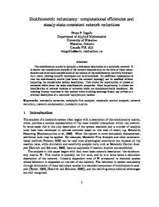
2. Compute M = πR.attr4 (T ); this is the magic set. 3. Join M with S, continue computing ∆2 ; call the result T2 . 4. group T2 by R.attr4 ; compute aggregate F (attr2 ). Call the result T3 . 5. Join T3 and T1 ; use a selection for the linking condition. In our approach, we consider the table containing the correlated attribute as part of the FROM clause of the subquery too (i.e. we effectively decorrelate the subquery). Thus, the outer join is always part of our common part. In our plan, there are two steps: 1. compute the base relation, given by g(∆1 ∩ ∆2 )(T ∪ {R, S}). This includes the outer join of R and S. 2. computation of a grouped forloop defined by F L(attr6, F (attr2), ∆2 − ∆1 , ∆1 − ∆2 ∧ attr1 θ F (attr2)) which computes the rest of the query. Dayal’s query plan and our query plan are shown as trees in Figure 4.2. Our plan has two main differences with Dayal’s: the parts common to query and subquery are computed only once, at the beginning of the plan, and computing the aggregate, the linking predicate, and possible some selections is carried out by the forloop predicate in one step. Thus, we potentially deal with larger temporary results, as some selections (those not in ∆1 ∩ ∆2 ) are not pushed down, but may be able to effect several computations at once (and do not repeat any computation). Compared to magic sets, a trade-off is quickly obvious: by fixing the common part, we do not repeat computations, but cannot separate the production of complementary and magic sets from the processing -since the common part is in both the complementary set and the subquery. Therefore, like Dayal’s approach, we may compute more aggregates in the subquery than the magic set approach. However, we do not generate additional joins or temporary tables and do not repeat computations. Clearly, which plan is better depends on the amount of redundancy between query and subquery, the linking condition (which determines how efficient the for-loop operator is), and traditional optimization parameters, like the size of the input relations and the selectivity of the different conditions.

4.3

Extensions

The presentation so far has limited for-loops to be applied to queries with aggregated subqueries, where the subquery and query have the same FROM clause. However, the approach can easily be generalized to more general cases. First, we point out that it is possible to rewrite any SQL query with a (non aggregated) subquery into a query with an aggregate subquery. For instance, it is well known that a condition like EXISTS Q, where Q is a subquery, can be transformed to the semantically equivalent 0 > Q’, where Q’ is a query derived from Q by changing Q’s SELECT clause from whatever it was to SELECT COUNT(*). The introduction of ’*’ is needed to deal with null values. Similar subtle transformations are needed in other cases. The point is, however, that all SQL subqueries can be rewritten similarly, as shown in [3]. Hence, the approach presented here can be applied to any SQL query with subqueries of any kind, by first rewriting the subquery and linking condition appropriately. Second, the approach can deal with situations where query and subquery have different FROM clauses as follows. Let T1 be the FROM clause of the main query and T2 the FROM clause of the subquery, and ∆1 and ∆2 are before. If T1 ∩ T2 = ∅, then nothing can be done with our approach. However, if T1 ∩ T2 6= ∅, we can still derive a common part as ∆1 ∩ ∆2 (T1 ∩ T2 )6 Let P1 = ∆1 ∩ ∆2 (T1 ∩ T2 ), P2 = ∆1 − ∆2 (T1 − T2 ) and P3 = ∆2 − ∆1 (T2 − T1 ). To compute the aggregate in the subquery we need P1 ./ P2 ; and to compute the linking condition and the final result we need P1 ./ P2 . However, if we join each part separately we cannot use the for-loop (which takes one relation as input), and we cannot use P = P 1 ./ P2 ./ P3 as the base 6 Note that, in the case of correlated subqueries, we add to T the relation in T which provides the correlated attribute, and 2 1 therefore all correlated subqueries are in this case.

14

Project(L)

Project(L)

Select(attr1 F(attr2)) FL(attr6,F(attr2),Delta2−Delta1,Delta1−Delta2^attr1 F(attr2)) Join

Select(Delta1)

GB(attr6,F(attr2))

T

Delta1 ^ Delta2

Select(Delta2)

T

Join OuterJoin

R

T

S (b)

(a)

Figure 1: Standard plan for NQ queries (a) vs. forloop plan (b) relation for the for-loop, since tuples in P1 are needed for computations both in query and subquery: if a tuple in P1 has a match in P2 but does not have a match in P3 it will disappear from P , even though it may be part of the final result; if a tuple in P1 has a match in P3 but does not have a match in P2 it will disappear from P , even though it is needed to compute the right aggregation in the subquery. The problem is that all tuples in P1 must be kept, but we need to know, for each such tuple, if it is part of the subquery only, the main query, or both. To understand the situation, imagine tables R, S, T and U as described below and the query SELECT R.A FROM R, S, T,Z WHERE R.B = S.C and S.D = T.E and T.F =Z.G and R.A = (SELECT SUM(S.D) FROM S,T,U WHERE R.B = S.C and S.D = T.E and T.F =V.I) R S T Z V A B C D E F G H I J 1 2 2 3 3 5 5 8 6 10 2 2 2 4 4 6 5 9 6 11 The common part is the join of R with S and T : R ./ S ./ T A B C D E F 1 2 2 3 3 5 1 2 2 4 4 6 2 2 2 3 3 5 2 2 2 4 4 6 15

After that, the join with Z will qualify rows 1 and 3 (starting at the top) of the above result; the value of R.A sent to the correlated attribute is 2, and it is sent twice. Clearly, then, R ./ S ./ T is the same for query and subquery. However, in the subquery a join with V will qualify rows 2 and 4, and the sum will be over values 4 and 4 of S.D. Clearly, we cannot throw away any row of the common part if we expect to compute the forloop on it; we can only “mark” each tuple as belonging to the outer query, the subquery or both7 . One way to accomplish this is to use outer joins instead of regular joins in P : we (left) outer join P 1 to P2 , and then (left) outer join the result to P3 . Tuples which have nulls in both the P2 and P3 parts of the schema can be disregarded; tuples that have nulls in P2 but not in P3 are considered for the computation of the aggregate but not for the result; and tuples that have nulls in P3 but not in P2 are considered for the result, but not for the computation of the aggregate (obviously, tuples with no nulls are considered for both computation of the aggregate and appearance in the result). This can be accomplished easily by adding a condition isnull(P1 .key) to ∆1 − ∆2 and a condition isnull(P2 .key) to ∆2 − ∆1 in the for-loop operator. If all selections are pushed down, and all attributes required in the for-loop come from relations in T 1 ∩T2 , all information needed is in P1 , and the outer joins with P2 and P3 are required basically to determine which tuples are in the main query and which are in the subquery part. A possible optimization then is to use semijoins in the definition of P . Unfortunately, a semijoin loses information about duplicates, and this information is needed to compute aggregates correctly in SQL (at least those aggregates that are duplicatesensitive ([])) and also to determine how many times a tuple must appear in the result, since SQL does not remove duplicates unless explicitly stated in the query (DISTINCT keyword). Thus, the semijoin strategy is not directly applicable. Our approach for this case is to join P1 to P2 and then to P3 using cardinal joins. Intuitively, a cardinal join of relations R and S tells us how many tuples in S match each tuple in R by creating a counter in each tuple in R with such information. Thus, let A ∈ sch(R), B ∈ sch(S), and let sch(R) = A1 , . . . , An . Then the cardinal join of R and S on condition AθB (in symbols R ./CAθB S) produces a relation of schema A1 , . . . , An , N, where N is a special domain isomorphic with the natural numbers. The cardinal join is defined as R ./CAθB S = {t | ∃t0 ∈ R ∧ t[R] = t0 ∧ t[N] =| {t00 | t00 ∈ S ∧ t0 .Aθt00 .B} |}. Then (P1 ./C P2 ) ./C P3 will add, to each tuple in P1 , two counters. If both are 0, the tuple can be ignored. If the counter created by P2 is set of 0, the tuple is ignore for computing the linking condition and the final result; if the counter created by P2 is set of 0, the tuple is ignore for computing the aggregate. Again, this can be accomplished easily by adding a condition (P1 .N1 = 0) to ∆1 − ∆2 and a condition (P2 .N2 = 0) to ∆2 − ∆1 in the for-loop operator. A comparison of our approach and the standard approach can be summarized as follows: • In the presence of correlation, our approach is similar to unnesting in Dayal’s style, in that query and subquery are (outer)joined through the correlation. Unlike magic sets, we cannot produce a minimal set of values for the correlation, as we start by identifying common parts that belong to both query and subquery. On the other hand, our approach avoids any duplicated work, and may be able to compute groupings, aggregations and some selections in one pass. Our approach cannot be applied when T1 ∩ T2 = ∅, i.e. query and subquery have nothing in common. • For non correlated queries, our approach degenerates to the standard approach when T 1 ∩ T2 = ∅. In this case, there is probably no other approach possible but the standard one (execute query and subquery separately). However, whenever some overlap exists, our approach may reduce the amount of work to be done, while the standard approach still executes query and subquery separately. • In all cases, our approach executes any common parts of query and subquery together. As pointed out, this may or may not be a good strategy, depending on the amount of overlap, and size of temporary relations created (i.e. selectivity factor of conditions and their distribution). There is a trade-off between fixing the order of execution of joins and selections and not repeating any work. 7 Contrast this with the magic set approach: R ./ S ./ T ./ Z would be computed and yield the complementary table; a projection on R.B would yield the magic set table; and a semijoin of this magic set with S ./ T ./ V would be used to compute the aggregates in the subquery. Thus, the number of computations in the subquery could potentially be reduced, at the cost of producing more temporary results and and additional join later in the plan. In particular, the join R ./ S ./ T is repeated.

16

4.4

Issues with nulls

The SQL standard shows some peculiarities in the handling of nulls. In order to respect SQL’s semantics, programs have to be extended to deal with nulls. In essence, when a null value is found in the computation for an aggregate, it should be ignored (except for the case of COUNT(*)). However, care must be taken in the program to avoid some programming mistakes. For instance, our variables mix, max, etc. are given an initial “dummy” value with the idea that they will be given a real value as soon as the iteration begins. But null values will make this variables remain in their “dummy” state, which in some cases will provoke an accumulation of values in the temporary result. Particularly, if all the values in an attribute are null, the variables remain in their “dummy” state, which may cause problem in the comparisons. Thus, when nulls are present, some computation may need to be postponed, and the program performance may degrade. Presence of nulls should be one of the factors that the optimizer takes into account when calculating the cost of a for-loop (i.e. whether the columns involved are declared as not null or not). In a data warehousing context, which is where we believe our alternative plan would be more useful, we assume that nulls have been cleaned out during the ETL (Extraction-Transformation-Loading) phase ([16]).

5

Cost Analysis

A typical for-loop query plan consists of a series of standard relational operations to compute the base relation and the for-loop itself. Thus, to estimate the cost of a for-loop query plan, simply add the cost of all operations needed to produce the base relation and then add the cost of the for-loop itself. The cost of the for-loop can be roughly approximated as follows (in the following, we do not include the cost of writing the output for further processing. In most cases considered so far, the for-loop is the last operation in the tree and its result could go directly to the required output). For the flat case, the program simply iterates over its input. If there is space for result in main memory, the cost is then basically that of a relation scan. Whether result can be reasonably expected to fit in main memory or not depends on several parameters, like physical memory size and data distribution. As stated above, for certain linking conditions and aggregates, it is more likely that result will fit into memory, since tuples can be promptly eliminated from consideration, while for other cases this is not so likely. If result does not fit into memory, part of it will have to be written back to disk and possibly retrieved at some point for filtering. One possible strategy is to distribute available memory in two buffers: an input buffer to read the relation in and a output buffer to store result. When the linking condition and aggregate favor early tuple selection, the memory is distributed with a bias towards the input buffer, allowing the system to scan the relation with sequential prefetch ([27]) and thus saving disk I/O. When the linking condition and aggregate are not so favorable, the memory may be distributed with a bias towards the output buffer, to maximize chances of keeping result in memory. Note that in some of the difficult cases, the tuples can be divided into for sure in the result and possibly in the result; in case of memory scarcity, we should write the for sure tuples to disk as they do not need to be retrieved again, thus making more room for the possibly set. Thus, it is likely that we can build result in memory and write it out to disk as we go without having to retrieve it back. In a worst-case scenario (for instance, when the aggregate is average), all tuples must be kept into memory and cannot be filtered until the end -in this case, it is simply better not to save anything in partial and revisit the base relation once the aggregate has been calculated. Thus, for an input relation with size N blocks, the average cost will be roughly N disk I/Os, but the worst-case cost is that of scanning the base relation twice -2N , the same as for standard relational processing. We note, however, that when selections are involved, a relational plan may add separate selection nodes, and therefore a double scan of the relation is a minimum cost for the relational processor, while the forloop essentially pipelines selections, thus taking care of them at no cost. For the case of the grouped for-loop, there is obviously the cost of grouping the relation, which dominates all other operations. In a direct implementation (which we are currently developing), an algorithm for grouping (i.e. hashing or sorting) is modified so that other operations in the for-loop program are done when the tuple is brought into memory for the grouping (we prefer hashing since it immediately tells us to which group a tuple belongs to). Result is implemented as an array with entries for each group, constructed off of the hash table. Once tuple t is hashed based on t.attr, other operations can be done. Typically there is a

17

computation that goes on for each group (with variables local to each group), so a small amount of memory is needed per group to hold temporary results. There may be other global variables needed, but the amount of memory is usually very small. We note that grouping operations usually reduce the size of the output relation, as the final result contains only one tuple per group. This is also true in our case, and therefore the global result may fit in memory. Thus, as far as temporary results (the array with local variables and partials for each group) can be kept in main memory, the cost of the grouping for-loop is basically the same as the cost of grouping the relation by hashing. Again, whether that is possible depends on some external parameters. In this case, data distribution plays an even greater role as the skewness of data may make some groups very large, and hence difficult to keep in memory (although this also means other groups will be very small; thus, distributing the memory dynamically among entries in the array may alleviate this problem). As before, some linking operators and aggregates make it more likely that the size of the partials for each group can be kept in check, while others make it less likely. Again as before, partitioning dynamically the memory between an input buffer and an output buffer for result (and dynamically partitioning this output buffer among the for sure and possibly tuples, whenever appropriate) may help. If we can keep all partials in memory, the cost for a relation of size N blocks will again be roughly N disk I/Os (recall that we do not count output write costs), but in a worst-case scenario (we must keep all tuples per group, all groups exceed the available memory and must be partially written to disk, and we have to retrieve all groups for further filtering), we read the relation twice and write it once -for a total cost of 3N . Compared to a traditional query plan, however, which may involve several selections and a grouping, this cost can be considered competitive. The decision to use a for-loop plan can, in principle, be decided on a series of factors: • the amount of redundancy or overlap between query and subquery. Obviously, the greater the overlap the more it is to be saved by executing that part of the query only once. Overlap can be defined as the repetitions of operations in the WHERE clause of query and subquery. The amount of overlap can be expressed as the fraction of the number of overlapping operations divided by the total number of (∆1 ∩∆2 ) ). In computing the overlap, we different operations in both WHERE clauses (i.e. as ∆1 ∪∆2∆1−∩∆ 2 should take into account the number of joins (as this is the most expensive operation) and, to a minor extent, the cost of selections. • the estimated size of the base relation. • the particular linking aggregate and linking condition, which determine, to a certain extent, the chances that result will be small enough to be kept in memory. Another factor that determines this is data distribution. However, neither one of these factors can determine in advance the cost of the for-loop plan alone. Size of relations, selectivity factors in selections in the common part and not in the common part, access paths and so on are a large part of the final cost of the plan. Therefore, to consider a for-loop plan, a cost-based optimizer should rely on the cost of the plan only. Thus, the optimizer should, if redundancy is present, construct a query plan with for-loops on it, and estimate the cost by traditional methods. Note that the size of the base relation will be produced as part of the standard estimate. Also, the influence of the particular linking aggregate and linking condition can be taken into account by multiplying the base cost of the for-loop (N ) by a factor determined by the aggregate and condition, giving the analytical chances that the result will be of bounded size. Such a table is outlined before, and it contains values between 1 (best case) and 3 (worst case), to adjust our cost estimates above. linking operator linking aggregate cost factor = min, max 1 = sum, count 1.5 < min 1.5 > max 1.5 > min 2 < min 2 any average 3

18

5.1

Example and Analytical Comparison

We apply our approach to query 2 of the TPC-H benchmark, shown in example 1. This is a typical NG query.

Select ps_supplycost=min(ps_supplycost) Join Join

GBps_partkey,min(ps_supplycost) Select size=15&type LIKE %BRASS

Join

Join Part

Select name="Europe"

Join

Select name="Europe"

Join Join

Region Nation

Region Join

PartSupp

Supplier PartSupp

Nation Supplier

Figure 2: Standard query plan For our experiment we created a TPC-H benchmark using two leading commercial DBMS. We filled the database to the smallest size, 1 GB. We used a Linux server with 512 Mg of RAM and several small SCSI disks on a RAID5 configuration. We created indices in all primary and foreign keys, updated system statistics, and then run query 2 on create plan mode, i.e. we asked the system for a query plan for the query. Each query plan was then extracted and interpreted. Both query plans were very similar, and they are represented by the query tree in figure 1. Note that the query is unnested based on Kim’s approach (i.e. first group and then join). Kim’s method is probably preferred over Dayal’s (first outerjoin, then group) as it tends to be more efficient (it groups first, reducing the size of relations before the join, and it uses a regular join, instead of an outerjoin) and it gives a correct translation for this query. Note also that all selections are pushed down until they are on top of the relations, where they are pipelined with the joins. The main differences between the two systems were the choices of implementations for the joins and different join ordering (for the case of the main query; the plans for the subquery were virtually identical). Also, one of the systems considered the join between part and partsupp (introduced by the unnesting) as a single join with two conditions (the one introduced by the correlation and the one introduced by the linking condition), while the other system preferred to express this situation as a (simple condition) join followed by a selection. However, the overall plan structure was the same in both cases. To make sure that the particular linking condition was not an issue, the query was changed to use different linking aggregates and linking operators; the query plan remained the same, except that for operators other than equality the join changed to an outerjoin and the grouping was done after the outerjoin. Also, memory size was varied from a minimum of 64 M to a maximum of 512 M, to determine if memory size was an issue. Again, the query plan remained the same through all memory sizes. For our concern, the main observation about this query plan is that operations in query and subquery are repeated, even though there clearly is a large amount of repetition. We have disregarded the final Sort needed to complete the query, as this would be necessary in any approach, including ours. We created a query plan for this query, based on our approach (shown in figure 2). Note that our 19

FL(p_partkey, min(ps_supplycost),

(p_size=15 & p_type LIKE %BRASS & ps_supplycost=min(ps_supplycost))

Join Join Part Join

Select name="Europe"

Region Nation PartSupp

Join Supplier

Figure 3: For-loop query plan approach does not dictate how the base relation is optimized; the particular plan shown uses the same tree as the original query tree to facilitate comparisons. By comparing the query plans, it is easy to see that our approach avoids any duplication of work. However, this comes at the cost of fixing the order of some operations (i.e. operations in ∆1 ∩ ∆2 must be done before other operations). In particular, some selections get pushed up because they do not belong into the common part. This means that the size of the relation created as input for the for-loop may be large. In this particular case, Query 2 in the 1 GB size database returns 460 rows, while the intermediate relation that the for-loop takes as input has 158,960 tuples. Thus, the cost of executing the for-loop may add more than other operations since it may have to deal with a larger input. However, grouping and aggregating in even this size relation took both systems about 10% of the time of the whole query8 . Another observation is that the duplicated operations do not take double the time: because of cache usage, some data needed is already present in memory when joins and selections are going to be computed a second time. In our experiments, we determined that calculating the common part takes about 60% of query time. Thus, clearly the second time around the operations are done faster. However, this can be attributed to the excellent main memory/database size ratio in our setup; with larger size databases this effect is likely to be diminished. Finally, we observe that in this particular case (with equality as linking condition and min as linking aggregate), our approach does well as the result set can be filtered on the fly; in other situations this may not be the case. Nevertheless, our approach avoids duplicated computation and does result in some time improvement (it takes about 70% of the time of the standard approach). In any case, it is clear that a plan using the for-loop is not guaranteed to be superior to traditional plans under all circumstances. Thus, it is very important to note that we assume a cost-based optimizer which will generate a for-loop plan if at least some amount of redundancy is detected, and will compare the for-loop plan to others based on cost. Ultimately, a for-loop plan will only be preferred if it is predicted to yield a lower cost than traditional alternatives -something that we expect will happen for the right combination of common and not common parts and linking predicates. In this sense, the following approach behaves similarly to that of [24].

6

Related Work

There is a large body of research in query optimization, as the problem has tremendous practical importance. The seminal paper by Kim ([17]) introduced the notion of unnesting and introduced the idea of transforming SQL queries that fit certain patterns. This work had some problems which were identified in [11]. Further work by Dayal ([7]) and others ([22]) solved these problems and deal not only with subqueries but also with grouping. This work in turn was generalized with the magic sets technique ([32, 31, 30, 29]). All these 8 This and all other data about time come from measuring performance of appropriate SQL queries executed against the TPC-H database on both systems. Details are left out for lack of space but are available on the technical report.

20

approaches do not address the specific problem we are dealing with: that of redundancy between query and subquery. None of the unnesting approaches looks for (and therefore, is able to detect) such redundancy. Also, some of the patterns we cover refer to queries containing non correlated subqueries that cannot be unnested (type J in Kim). The recent interest in data warehousing and decision support has motivated further work on aggregates ([14]). Once again, this work does not address the specific problem we present. However, some of the ideas of [14] are reintroduced in the present context, since computing the aggregate on the fly is somewhat similar to pushing down the GROUP BY operator. The work of [19] and [8] may seem similar to the one presented here in that expressions in a relational language are transformed into programs in an iterative programming language. However, in these approaches the focus is on translating the whole query into a database programming language and they do not deal with SQL: [19] takes as input a query execution plan, and [8] takes as input programs in O++, an object-oriented programming language that interacts with a database. The work in [25] and [26] deserves special mention because of the similarities with the research developed here. Both papers observe that the constraints of SQL do not allow the language to express many aggregatebased queries in a single query. The inefficiencies are also attributed to redundancy in the language, and an extension to SQL which would allow many aggregation-based queries to be expressed succinctly is proposed. An operator for the relational algebra is given that translates the SQL extension, and an algorithm to evaluate efficiently the new operator is provided. Some of the patterns developed here can be rewritten using this SQL extension by first unnesting the queries ([7]). In these cases, the algorithm proposed in [26] is very similar to the for-loop program that we provide, in that relations are first grouped and then aggregations are calculated in one pass, possibly on different levels (see example 3). However, the for-loop approach is more general, in the following sense: the semantics of the extensions in [26] can be simulated in the for-loop approach by using conditional expressions in which the computation of the aggregate is suitably restricted; patterns of type NG and GG are examples. However, the for-loop approach can also be used in queries where no grouping is present, and with subqueries, whereas the extension of [26] is restricted to SPJG (SPJ with GROUP BY) queries. The work of [9] is similar to the one presented here in that expressions in a relational language are transformed into programs in an iterative programming language. However, there are also some major differences. The source language of [9] is a query execution plan or QEP (i.e. a set of operators on tables which model operators for relational queries). The QEP is defined as the set of expressions formed by the primitives (scan table), (filter pred? set-of-tuples), (project project-list set-of-tuples), (ljoin join-pred set1 set2), where filter represents the relational selection operator and ljoin represents the nested-loop join. The only difference between tables and set-of-tuples is that tables reside on disk while set-of-tuples may reside on disk or in memory. Thus, scan is the only operator that accesses the base relations from the database. We note that this set of operators cannot represent nested queries unless the predicates allowed in filters allow whole queries9 . The translation takes over after a QEP has been generated for a given query, and transforms the set-oriented operators into programs that are tuple-oriented. The target language of [9] is a version of the lambda calculus, and includes variables, function expressions, and conditional expressions (assignments and loops are also included to simplify some programs, but are not strictly necessary). The tables and set of tuples are represented in the target language by streams. Seen as a programming language, this target language is directly executable by a physical database processor (i.e. a back-end). On the other hand, our approach starts with the SQL query, as one of our tenets is that for some queries the QEP that relational processors generate is inherently wasteful, and generates programs in a highly restricted language, which could either be executed by a back-end or could in turn be considered as source for further transformation. In particular, our language also has variables, assignments and conditional expressions, but no function definition (and therefore no recursion) and no looping. All the looping is limited to the for expression surrounding the body of the program. Therefore, our target language is severely more limited (the use of the map mechanism in [9] can be seen as another syntax for the idea of for loops, and indeed our programs would be implementable in such a system). Thus, the two approaches operate at a different level. Also, the transformations are different in character. That of [9] is general (i.e. they apply to 9 If subqueries are going to be unnested, a semijoin and an outerjoin operators are necessary in order to correctly capture the semantics of some SQL subqueries. But there operators are not provided in [9].

21

all expressions of the source language) and optimization is one step of the process which basically consists of applying a set of simplification rules. Our approach applies only to a subset of our target language, and the whole transformation process can be considered as a optimization process as the program generated is, generally, more efficient than its relational counterpart. Also, the approach of [9] aims at transforming the whole query into a program, while we leave in relational form a part of it that varies from query to query (the part that we called the basic relation) and include in our body loop only certain parts of the query. Since every operation on the QEP is recursively specified, the transformations of [9] produce one loop (or map expression) per each table that is used. On our approach, several loops may be hidden in the evaluation of the basic relation, so the relationship is not straightforward. Finally, because the transformations of [9] are general, patters with the two-pass problem are not identified and optimized. Furthermore, since the source language of [9] is QEP, at which level repetition has already been introduced, it is extremely doubtful that this approach can deal with the two-pass problem. It has been mentioned that many of the problems arising from the inability of SQL to express some questions with a single query have already been addressed by practitioners and the SQL standard body. While these approaches have their merits, it is doubtful whether they are useful from a performance point of view. The approach of building a stepwise solution is hampered by the fact that very little work has been done on optimizing groups of SQL queries. The work of ([23]) is a primary example. Intuitively, it develops the idea of discovering common subexpressions among groups of queries, executing them once and storing the results for reuse. However, in the present situation common subexpressions are not likely to appear as each view or table represents a different step (partial solution) toward the ultimate goal. Therefore applicability of this research is limited. Thus, the overhead of having views or temporary tables together with the fact that the system treats each query individually gives this approach a disadvantage 10 . The approach of adding more constructs to SQL makes a language which is already becoming large and complicated more so. This in turn makes the issue of optimizing queries that use such constructs (which is where the performance gain would come from, not just from having those constructs), a technically complex and challenging task. Our approach shows the relationship between these two solutions.

7

Conclusions and Further Research

We have argued that Decision-support SQL queries tend to contain redundancy between query and subquery, and this redundancy is not detected and optimized by relational processors. We have introduced a new optimization mechanism to deal with this redundancy, the for-loop operator, and an implementation for it, the for-loop program. We developed a transformation process that takes us from SQL queries to for-loop programs. A comparative analysis with standard relational optimization was shown. The for-loop approach promises a more efficient implementation for queries falling in the patterns given. For simplicity and lack of space, the approach is introduced here applied to a very restricted class of queries. However, we have already worked out extensions to widen its scope. Mainly, the approach can work with overlapping (not just identical) FROM clauses in query and subquery, and with different classes of linking conditions (predicates like [NOT] IN and [NOT] EXISTS) ([3]). We are currently working on a native implementation of the for-loop so that we can compare the approach time-wise with traditional query optimization. Such an implementation will allow the for-loop operator to benefit from direct access to the database’s cache and I/O manager. We are implementing a for-loop operator, and extending a query optimizer to generate for-loop query plans when redundancy is detected. Once our implementation is complete, in-depth experiments will allow us to understand more clearly the cost of a for-loop operator and the influence of different factors outlined in section 5. Clearly, the approach should be tested on queries with different degrees of overlap, different linking conditions, and different data distributions. 10 Since a relational database system may treat views in two completely different ways -materialized vs. virtual- the above statement should be justified in more detail. When a view is materialized, there is a notable overhead in the form of disk reads and writes, storage space, and administrative work to enter the view in the data dictionary of the database. If views are virtual, the final query must somehow be combined with the view definitions and is transformed into one complex relational algebra expression, which is hard to optimize and may contain redundancy. In either case, our experiments conclude that neither approach solves the performance gap.

22

We are also working on extending the approach in other directions (it should deal with nesting levels greater than 1, ideally in a manner similar to [7] or [22]) and studying the properties of the for-loop as an algebraic operator, i.e. its behavior with other operators (does it commute with selections? join?). One intriguing possibility is that of defining materialized views with for-loop-based query plans and studying issues of view reuse for query optimization, a popular topic of research in data warehousing ([14, 6, 21]). Finally, applicability to OQL, where the semantics is characterized by nested loops, should also be studied.

References [1] Abiteboul, S., Hull, R., Vianu, V. Foundations of Databases, Addison-Wesley, 1995. [2] Badia, A. and Niehues, M. Optimization of Sequences of Relational Queries in Decision-Support Environments, in Proceedings of DAWAK’99, LNCS n. 1676, Springer-Verlag. [3] Cao, Bin and Badia, A. Subquery Rewriting for Optimization of SQL Queries, submitted for publication. [4] Chaudhuri, S. ans Shim, K. Including Group-By in Query Optimization, in Proceedings of the 2th VLDB Conference, 1994. [5] Chaudhuri, S. ans Shim, K. An Overview of Cost-Based Optimization of Queries with Aggregates, Data Engineering Bulletin, 18(3), 1995. [6] Cohen, S., Nutt, W. and Serebrenik, A. Algorithms for Rewriting Aggregate Queries using Views, Proceedings of the Design and Management of Data Warehouses Conference, 1999. [7] Dayal, U. Of Nests and Trees: A Unified Approach to Processing Queries That Contain Nested Subqueries, Aggregates, and Quantifiers, in Proceedings of the VLDB Conference, 1987. [8] Fegaras, L. and Maier, D. Optimizing Queries Using an Effective Calculus, ACM TODS, vol. 25, n. 4, 2000. [9] Freytag, J. and Goodman, N. On the Translation of Relational Queries into Iterative Programs, ACM Transactions on Database Systems, vol. 14, no. 1, March 1989. [10] Galindo-Legaria, C. and Rosenthal, A. Outerjoin Simplification and Reordering for Query Optimization, ACM TODS, vol. 22, n. 1, 1997. [11] Ganski, R. and Wong, H. Optimization of Nested SQL Queries Revisited, in Proceedings of the ACM SIGMOD Conference, 1987. [12] Goel, P. and Iyer, B. SQL Query Optimization: Reordering for a General Class of Queries, in Proceedings of the 1996 ACM SIGMOD Conference. [13] Gray, J., Bosworth, A., Layman, A. and Pirahesh, H. DataCube: A Relational Aggregation Operator Generalizing Group By, Cross-Tab, and Sub-Totals. In Proceedings of the 12th IEEE ICDE, 1996. [14] Gupta, A., Harinayaran, V. and Quass, D. Aggregate-Query Processing in Data Warehousing Environments, in Proceedings of the VLDB Conference, 1995. [15] Hellerstein, J. Optimization Techniques for Queries with Expensive Methods, ACM TODS, vol. 23, n.2, 1998. [16] Jarke, M., Lenzerini, M., Vassiliou, Y. and Vassiliadis, P. Fundamentals of Data Warehousing, Springer-Verlag, 2000. [17] Kim, W. On Optimizing an SQL-Like Nested Query, ACM Transactions On Database Systems, vol. 7, n.3, September 1982.

23

[18] Kimball, R. What is wrong with decision support and how to fix it, SIGMOD Record, vol. 24, n. 3, September 1994. [19] Lieuwen, D. and DeWitt, D. A Transformation-Based Approach to Optimizing Loops in database Programming Languages, in Proceedings of the ACM SIGMOD Conference, 1992. [20] Lu, H., Chan, H. C. and Wei, K. K. A Survey on Usage of SQL, SIGMOD Record, 1993. [21] Materialized Views: Techniques, Implementations and Applications, A. Gupta and I. S. Mumick, eds., MIT Press, 1999. [22] Muralikrishna, M. Improving Unnesting Algorithms for Join Aggregate Queries in SQL, in Proceedings of the VLDB Conference, 1992. [23] Park, J. and Segev, A. Using common subexpressions to optimize multiple queries, in Proceedings of the 1988 IEEE CS ICDE. [24] Ross, K. and Rao, J. Reusing Invariants: A New Strategy for Correlated Queries, in Proceedings of the ACM SIGMOD Conference, 1998. [25] Ross, K. and Chatziantoniou, D., Querying Multiple Features of Groups in Relational Databases, in Proceedings of the 22nd VLDB Conference, 1996. [26] Ross, K. and Chatziantoniou, D., Groupwise Processing of Relational Queries, in Proceedings of the 23rd VLDB Conference, 1997. [27] O’Neill, P. and O’Neill, E. Database Principles, Programming, and Performance, Morgan Kaufmann, 2nd edition, 2001. [28] Jun Rao, Bruce Lindsay, Guy Lohman, Hamid Pirahesh and David Simmen, Using EELs, a Practical Approach to Outerjoin and Antijoin Reordering, in Proceedings of ICDE 2001. [29] Praveen Seshadri, Hamid Pirahesh, T. Y. Cliff Leung Complex Query Decorrelation, in Proceedings of ICDE 1996, pages 450-458. [30] Praveen Seshadri, Joseph M. Hellerstein, Hamid Pirahesh, T. Y. Cliff Leung, Raghu Ramakrishnan, Divesh Srivastava, Peter J. Stuckey, and S. Sudarshan Cost-Based Optimization for Magic: Algebra and Implementation, in Proceedings of the SIGMOD Conference, 1996, pages 435-446. [31] Inderpal Singh Mumick and Hamid Pirahesh Implementation of Magic-sets in a Relational Database System, in Proceedings of the SIGMOD Conference 1994, pages 103-114. [32] Inderpal Singh Mumick, Sheldon J. Finkelstein, Hamid Pirahesh and Raghu Ramakrishnan Magic is Relevant, in Proceedings of the SIGMOD Conference, 1990, pages 247-258. [33] TPC-H Benchmark, TPC Council, http://www.tpc.org/home.page.html.

24