Figure S1. Hierarchical average-linkage clustering of the samples ...

1

Figure S1. Hierarchical average-linkage clustering of the samples based on the Pearson’s

2

correlation coefficient of the abundance of oligotypes in the different samples. The color scale

3

indicates the scaled abundance of each variable: red, high abundance; blue, low abundance. The

4

upper column bar is colored according to the type of sample: red, cheese dataset; blue, meat dataset.

5

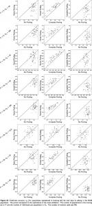
Figure S2. Correlation between oligotypes occurring in the cheese (panel a) and meat (panel b)

6

dataset. The bubbled text in each cell reports the p-value for that pairwise correlation. The color

7

scale indicates the level of correlation (red, positive correlation; blue, negative correlation) and the

8

cells are colored according to the correlation level. Tests were carried out using R (version 3.2.2)

9

considering the counts matrix for each oligotype. Significance (p value) was calculated using the

10

“corr” function, which employs a Student’s t distribution for a transformation of the correlation.

11

Bonferroni correction was used for multiple tests by multiplying significance estimates by 3152 ~=

12

105.

13

Figure S3. Co-occurrence between Pseudomonas oligotypes occurring in the cheese (panel a) and

14

meat (panel b) datasets. The bubbled text in each cell compares the number of samples in which

15

both oligotypes co-occurred (numerator) to the prevalence of the more abundant oligotype

16

(denominator). The color scale indicates the level of co-occurrence (purple; high number of co-

17

occurrence; yellow, low number of co-occurrence) and the cells are colored according to the co-

18

occurrence level. Tests were carried out using R (version 3.2.2) considering the counts matrix for

19

each oligotype. Two distinct indices (binary Jaccard: presence–absence, and Morisita-Horn: relative

20

abundance) estimated dissimilarity in pairwise comparisons of oligotypes sequences.

21 22 23 24 25 26 27 28 1

29

Figure S1

2

30

Figure S2

31 32 33 34 35 36 37 38 39 40 41 42 43 44 45 46 47 48 49 50 51 52 53 54 55 56 57 58 59 60 61 62 63 64 65 66 67 68

3

69

Figure S3

70 71 72 73 74 75 76 77 78 79 80 81 82 83 84 85 86 87 88 89 90 91 92 93 94 95 96 97 98 99 100 101 102 103 104 105 106 107

4

108

Table S1 A - Description of the food samples analyzed in this study.

109 Sample a Brine Caciocavallo* b Caciocavallo After moulding* b

Caciocavallo Curd pre-stretching**

b

Caciocavallo Surface t0** Caciocavallo Surface t10** b Caciocavallo Surface t20** b

b

Caciocavallo t0 * Caciocavallo t30* b Caciotta Curd** b Caciotta Surface 48h** b Caciotta Surface t20** b

c

Milk*

b

Grancacio* Mozzarella* b Ricotta* b Scamorza* b

d e

Carcass (A-E)***

A 1-5.t0*** e B 1-5. t0*** e C 1-5. t0*** f A 1-5.t6*** f B 1-5. t6*** f C 1-5. t6*** e A-W.Beef**** e A-X.Pork**** 110

Description Liquid brine used for salting of Caciocavallo cheese Caciocavallo cheese obtained after stretching and molding steps Curd obtained by coagulating milk and ready for stretching, molding and brining steps for Caciocavallo production Section of Caciocavallo cheese after stretching, molding and brining, ready to start the maturation process Section of Caciocavallo cheese after 10 days of ripening Section of Caciocavallo cheese after 20 days of ripening Caciocavallo cheese obtained after stretching, molding and brining, ready to start the maturation process Caciocavallo cheese after 30 days of ripening Curd obtained by coagulating milk addressed to Caciotta production Shallow section of Caciotta cheese after 48 hours of ripening Shallow section of Caciotta cheese after 20 days of ripening

Temperature (°C) 18 65

pH 6.97 5.64

aw 0.826 0.976

37

5.52

0.964

9 9 9

5.50 5.79 5.82

0.977 0.951 0.952

9 9 9 9 9

6.02 5.60 5.53 5.51 5.17

0.976 0.954 0.993 0.979 0.941

Pasteurized milk addressed to cheese production Pasta-filata cheese with production technology similar to Caciocavallo but characterized by larger size Mozzarella cheese Fresh, soft cheese, not fermented Pasta-filata cheese with a semi-soft texture and a typical pear shape Swab sampling of bovine carcasses performed 12 hours from slaughtering, after washing/before chilling Beef cuts from the butchery A were sampled immediately after portioning Beef cuts from the butchery B were sampled immediately after portioning Beef cuts from the butchery C were sampled immediately after portioning Beef cuts from the butchery A were sampled after 6 days of storage from portioning Beef cuts from the butchery B were sampled after 6 days of storage from portioning Beef cuts from the butchery C were sampled after 6 days of storage from portioning Beef cuts from the butchery were sampled immediately after portioning Pork cuts from the butchery were sampled immediately after portioning

71

6.71

0.990

9 9 9 9

5.63 5.22 5.71 6.13

0.916 0.995 0.984 0.945

7 4 4 4 4 4 4 4 4

6.81 5.44 5.72 5.32 6.61 7.11 6.93 5.24 5.11

0.995 9.983 0.985 0.986 0.908 0.912 0.918 0.986 0.985

(A detailed description of the samples is reported by Stellato et al., 2015(*); Calasso et al., 2015(**);De Filippis et al., 2013(***); Stellato et al., 2016(****)).

5

111

Table S1 B - Description of the sampling method in this study.

Sample a

Description

b

Representative section was sampled

c

Fifty ml of pasteurized milk were sampled by sterile vessel The carcass was sampled rubbing with sterile sponge swab vertically, horizontally and diagonally across the sampling site (100 cm2)

d

Fifty ml of liquid brine were sampled by sterile vessel

e

Fresh beef and pork cuts were sliced by knife and immediately analyzed once transferred to the laboratory

f

Beef and pork cuts were sliced by knife and immediately analyzed after 1 week of storage at 4°C

112

6

Tabella S2-A Relative abundance of Pseudomonas in the Cheese dataset samples.

 

Sample

Pseudomonas abundance (%)

Sample

Pseudomonas abundance (%)

1S_Vat

2.51

2S_Stretcher2

0.26

1S_Tank.Curd

15.82

2S_Molder2

64.01

1S_Curd.Bench

37.15

2S_Tank.Scamorza

28.75

1S_Knife.Curd

19.32

2S_Tank.Ricotta

3.36

1S_Dipper

32.53

2S_Mold.Ricotta

45.43

1S_Hand

16.29

2S_Mold.Mozzarella

0.15

1S_Chopper

77.98

2S_Mold.Grancacio

2.46

1S_Stretcher

36.06

2S_Rope

24.46

1S_Molder

31.07

2S_Hook.t0

0.11

1S_Chopper2

8.13

2S_Hook.t30

1.13

1S_Stretcher2

75.26

3S_Stretcher

0.11

1S_Molder2

12.24

3S_Floor

0.23

1S_Tank.Scamorza

70.53

Ricotta

29.88

1S_Mold.Ricotta

19.15

Mozzarella

4.84

1S_Mold.Mozzarella

39.96

Grancacio

4.13

1S_Mold.Grancacio

66.24

Brine.Caciocavallo

5.03

1S_Rope

16.58

1S_Brine.Caciocavallo

8.59

1S_Hook.t0

1.54

Caciocavallo.Aftermoulding

0.72

1S_Hook.t30

1.89

Caciocavallo.t0

0.32

2S_Vat

10.75

Caciocavallo.t30

0.09

2S_Tank.Curd

25.96

Cacio.Curd.Prestretching

0.05

2S_Curd.Bench

42.11

Caciotta.Curd

0.84

2S_Dipper

17.35

Caciotta.Surface.48h

0.11

2S_Hand

31.43

Caciocavallo.Surface.t0

0.14

2S_Chopper

23.91

Caciocavallo.Surface.t10

0.21

2S_Stretcher

19.55

Caciocavallo_Surface.t20

1.26

2S_Molder

29.02

Caciotta_Surface.t20

0.05

2S_Chopper2

11.36

Milk

0.49

Table S2-B Tabella S2-A Relative abundance of Pseudomonas in the meat samples.    

 

Sample

Pseudomonas abundance (%)

Sample

Pseudomonas abundance (%)

Sample

Pseudomonas abundance (%)

Carcass.A

1.47

B1.t6

50.76

T.Beef

34.5

Carcass.B

1.64

B2.t6

61.15

U.Beef

36.77

Carcass.C

0.83

B3.t6

59.17

V.Beef

19.62

Carcass.D

0.21

B4.t6

33.44

X.Beef

70.76

Carcass.E

1.14

B5.t6

16.82

W.Beef

64.35

A1.t0

7.15

C1.t6

62.51

A.Pork

29.35

A2.t0

2.71

C2.t6

46.82

B.Pork

42.34

A3.t0

4.49

C3.t6

66.76

C.Pork

23.07

A4.t0

3.84

C4.t6

17.95

D.Pork

17.71

A5.t0

2.17

C5.t6

28.76

E.Pork

27.92

B1.t0

2.39

A.Beef

51.48

F.Pork

26.99

B2.t0

22.87

B.Beef

26.81

G.Pork

19.05

B3.t0

26.69

C.Beef

52.6

H.Pork

63.86

B4.t0

34.57

D.Beef

49.01

I.Pork

54.96

B5.t0

33.64

E.Beef

18.59

J.Pork

42.13

C1.t0

46.81

F.Beef

40.34

K.Pork

27.92

C2.t0

63.15

G.Beef

57.15

L.Pork

21.8

C3.t0

41.45

H.Beef

54.96

M.Pork

60.99

C4.t0

39.59

I.Beef

54.91

N.Pork

44.39

C5.t0

0.48

J.Beef

62.62

P.Pork

69.45

A1.t6

75.33

K.Beef

47.7

T.Pork

27.57

A2.t6

76.66

L.Beef

20.43

U.Pork

35.33

A3.t6

67.46

M.Beef

40.45

V.Pork

16.32

A4.t6

48.47

N.Beef

34.39

W.Pork

20.92

A5.t6

34.69

S.Beef

14.62

X.Pork

20.79

Table S2-C Relative abundance of Pseudomonas in the meat dataset: environmental samples.   Pseudomonas abundance (%)

Sample

A.Chopping.Board

6,26

H.Knife

8,45

T.Hand

27,34

A.Hand

20,97

I.Chopping.Board

56,23

T.Knife

34,21

A.Knife

8,16

I.Hand

16,24

U.Chopping.Board

42,84

B.Chopping.Board

11,84

I.Knife

43,51

U.Hand

54,9

B.Hand

23,87

J.Chopping.Board

46,07

U.Knife

32,22

B.Knife

8,16

J.Hand

47,17

V.Chopping.Board

16,86

C.Chopping.Board

11,84

J.Knife

80,93

V.Hand

16,72

C.Hand

8,11

K.Chopping.Board

12,32

V.Knife

46,68

C.Knife

3,43

K.Hand

44,86

W.Chopping.Board

59,14

D.Chopping.Board

50,23

K.Knife

12,29

W.Hand

53,68

D.Hand

43,54

L.Chopping.Board

23,58

W.Knife

84,79

D.Knife

38,85

L.Hand

12,24

X.Chopping.Board

31,3

E.Chopping.Board

14,31

L.Knife

9,43

X.Hand

34,17

E.Hand

11,06

M.Chopping.Board

74,41

X.Knife

30,75

E.Knife

11,54

M.Hand

46,49

Y.Chopping.Board

0,55

F.Chopping.Board

17,46

M.Knife

65,03

Y.Coldstore

1,94

F.Hand

5,92

N.Chopping.Board

12,6

Y.Hand

6,16

F.Knife

20,28

N.Hand

12,24

Y.Knife

13,44

G.Chopping.Board

8,67

N.Knife

19,55

Z.Chopping.Board

2,45

G.Hand

8,84

S.Chopping.Board

14,33

Z.Coldstore

14,07

G.Knife

29,34

S.Hand

42,53

Z.Hand

6,61

H.Chopping.Board

14,34

S.Knife

22,45

Z.Knife

25,36

H.Hand

28,22

T.Chopping.Board

27,33

Sample

 

Pseudomonas abundance (%)

Sample

Pseudomonas abundance (%)