Filterable Particulate Matter Stack Test Methods

Filterable Particulate Matter Stack Test Methods: Performance Characteristics and Potential Improvements 3002000975

10061786

10061786

Filterable Particulate Matter Stack Test Methods: Performance Characteristics and Potential Improvements 3002000975 Technical Update, December 2013

EPRI Project Manager N. Goodman

ELECTRIC POWER RESEARCH INSTITUTE 3420 Hillview Avenue, Palo Alto, California 94304-1338 ▪ PO Box 10412, Palo Alto, California 94303-0813 ▪ USA 800.313.3774 ▪ 650.855.2121 ▪ [email protected] ▪ www.epri.com 10061786

DISCLAIMER OF WARRANTIES AND LIMITATION OF LIABILITIES THIS DOCUMENT WAS PREPARED BY THE ORGANIZATION(S) NAMED BELOW AS AN ACCOUNT OF WORK SPONSORED OR COSPONSORED BY THE ELECTRIC POWER RESEARCH INSTITUTE, INC. (EPRI). NEITHER EPRI, ANY MEMBER OF EPRI, ANY COSPONSOR, THE ORGANIZATION(S) BELOW, NOR ANY PERSON ACTING ON BEHALF OF ANY OF THEM: (A) MAKES ANY WARRANTY OR REPRESENTATION WHATSOEVER, EXPRESS OR IMPLIED, (I) WITH RESPECT TO THE USE OF ANY INFORMATION, APPARATUS, METHOD, PROCESS, OR SIMILAR ITEM DISCLOSED IN THIS DOCUMENT, INCLUDING MERCHANTABILITY AND FITNESS FOR A PARTICULAR PURPOSE, OR (II) THAT SUCH USE DOES NOT INFRINGE ON OR INTERFERE WITH PRIVATELY OWNED RIGHTS, INCLUDING ANY PARTY'S INTELLECTUAL PROPERTY, OR (III) THAT THIS DOCUMENT IS SUITABLE TO ANY PARTICULAR USER'S CIRCUMSTANCE; OR (B) ASSUMES RESPONSIBILITY FOR ANY DAMAGES OR OTHER LIABILITY WHATSOEVER (INCLUDING ANY CONSEQUENTIAL DAMAGES, EVEN IF EPRI OR ANY EPRI REPRESENTATIVE HAS BEEN ADVISED OF THE POSSIBILITY OF SUCH DAMAGES) RESULTING FROM YOUR SELECTION OR USE OF THIS DOCUMENT OR ANY INFORMATION, APPARATUS, METHOD, PROCESS, OR SIMILAR ITEM DISCLOSED IN THIS DOCUMENT. REFERENCE HEREIN TO ANY SPECIFIC COMMERCIAL PRODUCT, PROCESS, OR SERVICE BY ITS TRADE NAME, TRADEMARK, MANUFACTURER, OR OTHERWISE, DOES NOT NECESSARILY CONSTITUTE OR IMPLY ITS ENDORSEMENT, RECOMMENDATION, OR FAVORING BY EPRI. THE FOLLOWING ORGANIZATION, UNDER CONTRACT TO EPRI, PREPARED THIS REPORT: Clean Air Engineering, Inc.

This is an EPRI Technical Update report. A Technical Update report is intended as an informal report of continuing research, a meeting, or a topical study. It is not a final EPRI technical report.

NOTE For further information about EPRI, call the EPRI Customer Assistance Center at 800.313.3774 or e-mail [email protected]. Electric Power Research Institute, EPRI, and TOGETHER…SHAPING THE FUTURE OF ELECTRICITY are registered service marks of the Electric Power Research Institute, Inc. Copyright © 2013 Electric Power Research Institute, Inc. All rights reserved.

10061786

ACKNOWLEDGMENTS The following organization, under contract to the Electric Power Research Institute (EPRI), prepared this report: Clean Air Engineering, Inc. 500 W. Wood Street Palatine, Illinois 60067 Principal Investigators S. Evans W. Mills, PhD This report describes research sponsored by EPRI.

This publication is a corporate document that should be cited in the literature in the following manner: Filterable Particulate Matter Stack Test Methods: Performance Characteristics and Potential Improvements. EPRI, Palo Alto, CA: 2013. 3002000975. iii 10061786

10061786

ABSTRACT Fossil fuel-fired power plant owners are required to measure filterable particulate matter (fPM) in stack gases in order to comply with air permits that place limits on their emissions. Recent rulemakings by the U.S. Environmental Protection Agency (EPA) have given power plant owners the option to comply with emission limits for non-mercury metals classified as hazardous air pollutants (HAPs) by measuring fPM as a surrogate parameter. Compliance can be demonstrated either by quarterly sampling using a manual stack test method (for existing power plant units) or by using a particulate continuous emission monitor (CEM) or continuous parameter monitoring system (CPMS). Any of these options require measurement of fPM by manual stack test methods, as those will be used to calibrate the continuous monitors. The stack test method used most frequently to measure fPM for compliance with U.S. air permit limits is EPA Method 5. At low emission levels, the sensitivity and reliability of this method sets a lower limit on the calibration range of continuous monitors. Factors contributing to poor method performance include inappropriate sampling practices, background from sampling train rinses, filter variability and breakage, gas absorption on filter material, and uncertainties associated with the filter drying and weighing steps. A concerted effort is needed to identify and educate power companies that employ stack testers on approaches to minimize these uncertainties and biases. This report gathers available information on sources of uncertainty that impact the sensitivity and bias of the following methods for measuring fPM in stationary sources: EPA Methods 5, 17, and 201A. The report evaluates existing information on sampling and laboratory work practices as well as sampling train and laboratory equipment and materials to identify improvements that are expected to improve the precision of the method. Results of an uncertainty analysis of Method 5 are presented, and the implications of the analysis are discussed in relation to the use of the method for sources with low particulate emissions. Keywords Particulate matter PM filterable PM stack test methods air emissions

10061786

v

10061786

EXECUTIVE SUMMARY The ability to reliably measure low levels of particulate emissions from combustion sources such as fossil fuel-fired power plants has become increasingly critical due to the recent promulgation of more restrictive emissions limits by the U.S. Environmental Protection Agency (EPA). The purpose of this report is to evaluate available information on the performance of the standard EPA methods for measuring filterable particulate matter (fPM): EPA Methods 5, 17, and 201A. The report identifies the uncertainty and biases of measurement system parameters with the greatest impact on measurement quality, determines whether these methods can be applied with adequate precision and low bias at current and proposed emission limits, and recommends method enhancements that could extend the usefulness of the methods to sources with lower fPM emissions. The stack test method used most frequently to measure fPM for compliance with U.S. air permit limits is EPA Method 5, which employs an out-of-stack heated filter. The precision of this method at low concentrations sets a lower limit on the calibration range of continuous particulate monitors. Method 17 is an in-stack method that can only be used at plant units with dry stacks (i.e., those without a wet flue gas desulfurization system). Method 201A is used to speciate fPM into size fractions such as PM10 or PM2.5, and also can only be used on units with dry stacks. Previous studies of fPM methods show significant variability in method performance between stack testing companies and even between test teams from the same company. Factors contributing to poor method performance include loose specifications in the method, vague method language leading to inconsistent application, inappropriate sampling practices, contamination from sampling train rinses and other sources, filter variability and breakage, gas absorption on filter material, and uncertainties associated with the filter drying and weighing steps. A concerted effort is needed to develop approaches to minimize these uncertainties and biases. An uncertainty model was developed for Method 5 that incorporates estimates of the uncertainties of all measurements that go into calculating a fPM mass emission rate – moisture content of the gas stream, stack temperature, velocity, particulate mass, etc. The model then propagates these individual measurement uncertainties to the final mass emission result. Findings A review of previous studies and the results from the uncertainty analysis lead to the following findings: •

Previous studies on Method 5 uncertainty have been conducted at facilities with mass emission rates similar to the emission limits specified in the MATS rule for existing coalfired power plant units. These studies indicate that the method may be capable of producing results to better than 10% relative standard deviation (RSD) at those levels with reasonable sampling times. However, below the limit for new/reconstructed coal units of 0.009 lb/mmBtu, there are no data demonstrating method performance. The previous studies did not estimate precision below emission levels required to be met by new/reconstructed coal-fired plants or several other source categories.

10061786

vii

•

Uncontrolled bias effects have a far greater potential to adversely affect method performance than factors affecting method precision. Quality control and method improvement efforts should focus first on eliminating or reducing potential bias.

•

Positive biases may occur in Method 5 due to absorption of acid gases on glass fiber filters and effects of changing relative humidity on filter weights. These biases are significant and may exceed the true fPM at sites with very low emissions. Biases in Method 17 and 201A, which do not use an out-of-stack filter, have not been studied.

•

The total filterable particulate mass (TfPM) collected during the test drives method uncertainty for power plant testing. The sampling process is the predominant source of method uncertainty when TfPM is greater than about 10 mg. Below about 5 mg, analytical uncertainty predominates.

•

The minimum fPM mass necessary to collect during a test run in order to achieve reliable mass emission results is a function of 1) the gravimetric detection limit of the laboratory and, 2) the expected fPM concentration in the stack. A simple three-step process was presented to calculate the sampling time needed to collect the minimum fPM mass.

•

Acceptable Method 5 precision (±10% RSD) may be achieved with a one-hour test at mass emission rates as low as 0.001 to 0.002 lb/MMBtu with good quality control in the field and in the lab, tighter method specifications, stringent procedures to eliminate or minimize bias and a trained and experienced test team. The duration needed for a Method 201A test would be longer since the total particulate collected is divided between the two cyclones and the filter. How much longer is dependent upon the particle size distribution of the gas stream tested. In order to avoid gravimetric non-detects, the particulate mass collected on each cyclone analyzed as well as the filter must be above the minimum catch as calculated in this report.

Recommendations The report makes the following recommendations for using the existing test methods in order to minimize method uncertainty and bias for a given test: •

Use the most experienced and well-trained test crew possible.

•

When developing qualifications for testing firms, consider requiring third party accreditation.

•

Ensure the crew is diligent about minimizing possible sources of contamination and bias.

•

Always check stack diameter and cyclonic flow for each test. Do not rely on past measurements.

•

Ensure that the method enhancements described below are used.

•

Use reagent and train blanks to detect possible bias issues.

•

Conduct sample recovery in as clean an environment as possible.

10061786

viii

•

Send the samples to a laboratory with proven and documented performance in fPM sample analysis. Consider requiring third party accreditation.

Method Enhancements The findings of this report suggest that certain enhancements to both the sampling and analytical portions of the method may reduce uncertainty and bias and provide more reliable results at low fPM concentrations. Sampling Enhancements • Tighten the probe and filter temperature specification from the current ± 25°F to ± 10°F • Use only wind tunnel calibrated pitot tubes to obtain a more accurate pitot coefficient (C p ). Re-establish the coefficient after each test before the next field use. • Tighten isokinetic specification from ±10% on the run average to ±5% on each sampling point. Use quartz filters rather than glass, particularly when sampling gas streams containing reactive gases (such as coal-fired utility boilers). • Use only quartz or glass nozzle and liner whenever possible. • Specify equipment and procedures to perform a cyclonic flow check and require the check for all tests. • Use continuous electronic data collection for stack flow measurement rather than onceper-point manual data recording. • Collect a proof blank of at least one sampling train after sample recovery to detect potential bias issues. • Use new gloves for each sample recovery. • Use new probe and nozzle wash brushes for each run. • Use only well-trained and experienced testers. Check to see whether your test contractor is accredited by the Stack Testing Accreditation Council (STAC). While accreditation is no guarantee of quality work, it may improve the odds particularly when one is dealing with a new or unfamiliar contractor. Analytical Enhancements • Tare filters immediately before use to avoid humidity-induced bias. • Ensure that the laboratory employs rigorous static control procedures. • Tighten the Method 5 specification for “constant weight” from ± 0.5 mg to ± 0.3 mg or lower if possible. • Use Teflon beaker liners or other low weight sample containers to minimize tare weights. • Use a five place balance (0.00001 g) to weigh samples where possible. This has only a minor impact on uncertainty, however. The results of an analysis conducted by Clean Air Engineering show that a 4-place balance underestimates the variability of the gravimetric measurement compared to a 5-place balance. However, this effect is slight, amounting to a maximum of only 1% with extremely small filter loadings. •

Use only laboratories that conduct performance evaluations for filter analysis, such as method detection limit studies and blind Performance Test (PT) audits. Typically, these labs

10061786

ix

will be accredited through the National Environmental Laboratory Accreditation Program (NELAP) or other third party accrediting body. Reporting Enhancements • Require that the following information be included in the test report: filter type and manufacturer, date of tare, laboratory temperature and RH. This provides information to track down and resolve bias issues. Sensitivity of fPM Methods at Low Particulate Emissions Levels The results of the uncertainty analysis indicate that adequate precision (±10% RSD) can be achieved for Method 5 with a total particulate mass for a sample of about 6 mg. By implementing the enhancements and quality control improvements listed above, the minimum mass can be reduced to about 2 mg and still maintain the same precision, since the gravimetric measurement is the predominant source of uncertainty at very low particulate loadings. These measures may have a significant impact on the length of test runs required for very low concentration sources. However, the ability to quantify fPM reliably at such low levels assumes that method biases can be reduced to the point that they do not contribute significantly. Further research is needed to identify and minimize method bias. To the extent that uncertainties are known, similar conclusions can be made for Methods 17 and 201A; however, no comprehensive multi-train field studies have been completed on those methods.

10061786

x

SI CONVERSION FACTORS English (US) units

X

Factor

=

SI units

Area:

1 ft2

X

9.29 x 10-2

=

m2

Flow Rate:

1 gal/min

X

6.31 x 10-5

=

m3/s

1 gal/min

X

6.31 x 10-2

=

L/s

1 ft

X

0.3048

=

m

1 in

X

2.54

=

cm

1 yd

X

0.9144

=

m

1 lb

X

454

=

g

1 lb

X

0.454

=

kg

1 gr

X

0.0648

=

g

1 ton

X

0.907

=

tonne

1 ft3

X

28.3

=

L

3

1 ft

X

0.0283

=

m3

1 gal

X

3.785

=

L

Length:

Mass:

Volume:

1 gal

X

3.785 x 10

=

m3

Temperature:

°F-32

X

0.556

=

°C

Energy:

Btu

X

1055.1

=

Joules

Btu/hr

X

0.29307

=

Watts

10061786

-3

xi

10061786

ACRONYMS AND ABBREVIATIONS ASTM

American Society for Testing and Materials

Btu

British thermal unit

CEMS

continuous emissions monitoring system

CPMS

continuous parameter monitoring system

EGU

electric generating unit

EPA

U.S. Environmental Protection Agency

EPRI

Electric Power Research Institute

fPM

filterable particulate matter

MATS

Mercury and Air Toxics Standards Rule

MW

megawatt

NIST

National Institute of Standards and Technology

PM

particulate matter

PRB

Powder River Basin

RSD

relative standard deviation

SI

International System of Units

TfPM

total filterable PM

10061786

xiii

10061786

CONTENTS 1 INTRODUCTION ..................................................................................................................1-1 Scope of the Report ...........................................................................................................1-1 Regulatory Drivers for fPM Method Improvement ...............................................................1-2 EPA Reference Methods for Filterable Particulate Matter (fPM) .........................................1-5 Method 5 ......................................................................................................................1-5 Method 17 ....................................................................................................................1-7 Method 201A ................................................................................................................1-8 Overview of fPM Concentration and Mass Emissions Determination................................1-10 Method Performance Terminology ...................................................................................1-10 Accuracy, Precision, and Bias ....................................................................................1-11 Quantifying Uncertainty: What Does ± Mean? ............................................................1-12 Discussion of Detection and Quantitation Limits for fPM Methods ..............................1-13 2 EVALUATING TEST METHOD UNCERTAINTY ..................................................................2-1 Top Down Analysis ............................................................................................................2-1 Top Down Studies of Method 5 ....................................................................................2-1 Bottom Up Analysis ............................................................................................................2-8 Benefits and Limitations of the Bottom Up Approach ..................................................2-15 Additional Insights from the Bottom Up Analysis.........................................................2-16 Error Apportionment .........................................................................................................2-20 Process to determine minimum sampling time for a fPM Method................................2-23 Reducing Method Uncertainty ....................................................................................2-25 3 IDENTIFYING SOURCES OF METHOD BIAS .....................................................................3-1 Bias Sensitivity Analysis .....................................................................................................3-1 Group 1 – Stack Diameter (D s ) ...........................................................................................3-5 Group 2 – Volume, mass, and coefficients (V m , m n , Y d , C p ) ................................................3-5 Group 3 – Pressure (∆p, P bar ) ...........................................................................................3-12 Group 4 – Temperature and moisture (T s , T m , B w ) ............................................................3-13 4 FINDINGS AND RECOMMENDATIONS ..............................................................................4-1 Findings .............................................................................................................................4-1 Recommendations .............................................................................................................4-2 Method Enhancements ......................................................................................................4-2 Sampling Enhancements ..............................................................................................4-2 Analytical Enhancements .............................................................................................4-3 Reporting Enhancements .............................................................................................4-3 Sensitivity of fPM Methods at Low Particulate Emissions Levels ..................................4-3 5 BIBLIOGRAPHY ..................................................................................................................5-1 Referenced Sources...........................................................................................................5-1 Additional Resources .........................................................................................................5-2

10061786

xv

A METHOD DESCRIPTIONS ................................................................................................. A-1 B MEASUREMENT TERMINOLOGY ..................................................................................... B-1 Uncertainty/Error ............................................................................................................... B-1 Random Error/Precision/Repeatability/Reproducibility....................................................... B-2 Systematic Error or Bias .................................................................................................... B-3 Detection and Quantitation Limits ...................................................................................... B-4 Gravimetric Detection Limit.......................................................................................... B-4 Stack Test Method Detection Limits ............................................................................ B-6 C UNCERTAINTY ANALYSIS ................................................................................................ C-1

10061786

xvi

LIST OF FIGURES Figure 1-1 Effect of Particulate Measurement Bias on Mass Emission Rates .......................... 1-3 Figure 1-2 EPA Method 5 Sampling Apparatus ....................................................................... 1-6 Figure 1-3 EPA Method 17 Sampling Apparatus ..................................................................... 1-8 Figure 1-4 EPA Method 201A Sampling Apparatus ................................................................. 1-9 Figure 1-5 Determination of Mass Emissions (lb/hr) .............................................................. 1-10 Figure 2-1 Particulate Concentration vs. Relative Standard Deviations of fPM in Historical Studies .................................................................................................................................... 2-3 Figure 2-2 EPA Method 5 Collaborative Study Results (Hamil 3 Data) .................................... 2-4 Figure 2-3 EPA Method 5 Collaborative Study (Hamil 2 Data) ................................................ 2-5 Figure 2-4 EPA Method 5 Collaborative Study (Rigo, 1999 Data) ........................................... 2-6 Figure 2-5 Input Parameters for V mstd ....................................................................................... 2-9 Figure 2-6 Input Parameters for Q std ...................................................................................... 2-11 Figure 2-7 Input Parameters for m n ....................................................................................... 2-13 Figure 2-8 Relative Uncertainty as a Function of fPM Mass Collected .................................. 2-18 Figure 2-9 Relative Uncertainty as a Function of fPM Mass Collected (Low Masses)............ 2-19 Figure 2-10 Changes in Error Apportionment as a Function of fPM Mass – Area Plot ........... 2-21 Figure 2-11 Changes in Error Apportionment as a Function of fPM Mass – Line Plot............ 2-22 Figure 3-1 Particulate Sampling Method Sensitivity Analysis .................................................. 3-4 Figure 3-2 Pall Quartz Filter Environmental Effects Analysis ................................................... 3-7 Figure 3-3 Whatman Quartz Filter Environmental Effects Analysis.......................................... 3-8 Figure 3-4 Whatman Glass Filter Environmental Effects Analysis ........................................... 3-8 Figure 3-5 Collection Efficiency as a Function of Particle Size and Isokinetic Rate ............... 3-10 Figure A-1 EPA Method 5 Sampling Train............................................................................... A-1 Figure A-2 EPA Method 5 Specifications................................................................................. A-2 Figure A-3 EPA Method 5 Glassware Preparation .................................................................. A-3 Figure A-4 EPA Method 5 Sample Recovery .......................................................................... A-5 Figure A-5 EPA Method 5 Analytical Flowchart ....................................................................... A-6 Figure A-6 EPA Method 17 Sampling Train............................................................................. A-6 Figure A-7 EPA Method 17 Specifications............................................................................... A-7 Figure A-8 EPA Method 17 Glassware Preparation ................................................................ A-8 Figure A-9 EPA Method 17 Sample Recovery Flowchart ...................................................... A-10 Figure A-10 EPA Method 17 Analytical Flowchart ................................................................. A-11 Figure A-11 EPA Method 201A Sampling Train .................................................................... A-12 Figure A-12 EPA Method 201A Specifications ...................................................................... A-13 Figure A-13 EPA Method 201A Glassware Preparation ........................................................ A-14 Figure A-14 EPA Method 201A Sample Recovery ................................................................ A-15 Figure A-15 EPA Method 201A Analytical Flowchart ............................................................. A-16 Figure B-1 Frequency Distributions of Individual Filter Weights ............................................... B-5 Figure B-2 Frequency Distributions of Consecutive Day Net Filter Weights (Dec. – Apr.) ....... B-6

10061786

xvii

10061786

LIST OF TABLES Table 1-1 Summary of MATS Rule fPM Emission Limits for New and Existing Units .............. 1-4 Table 1-2 Summary of fPM AP-42 Emission Factors for Gas Turbines ................................... 1-5 Table 1-3 Example fPM Stack Concentrations Over Five Runs............................................. 1-12 Table 1-4 Uncertainty Expressed in Various Ways................................................................ 1-12 Table 2-1 Summary of EPA Method 5 Precision Estimates ..................................................... 2-7 Table 2-2 Directly Measured Parameters Used in V mstd Calculation.......................................... 2-9 Table 2-3 Intermediate Values Used in V mstd Calculation ....................................................... 2-10 Table 2-4 Final Result Calculations for V mstd .......................................................................... 2-10 Table 2-5 Directly Measured Parameters Used to Calculate Q std ........................................... 2-12 Table 2-6 Intermediate Values Used in Q std Calculation ......................................................... 2-12 Table 2-7 Final Result Calculations for V mstd .......................................................................... 2-13 Table 2-8 Directly Measured Parameters Used to Calculate m n ............................................ 2-14 Table 2-9 Intermediate Values Used in m n Calculation .......................................................... 2-14 Table 2-10 Final Result Calculations for m n .......................................................................... 2-14 Table 2-11 Three Components for Final Mass Emission Rate............................................... 2-15 Table 2-12 Final Calculated Results for Mass Emission Rate ............................................... 2-15 Table 2-13 Bottom Up Certainty Model Example................................................................... 2-16 Table 2-14 Additional Model Estimates ................................................................................. 2-17 Table 2-15 Final Mass Contribution Uncertainty at High fPM Levels ..................................... 2-20 Table 2-16 Minimum fPM Mass Needed to Achieve Desired Confidence in Final Mass Emission Rate ....................................................................................................................... 2-23 Table 3-1 Sensitivity Analysis Results ..................................................................................... 3-2 Table 3-2 Sensitivity Factor Summary (Normalized)................................................................ 3-3 Table C-1 Uncertainty Model Case Descriptions ..................................................................... C-1 Table C-2 List of All Directly Measured Parameters: Case 1 – Coal Fired Power Plant ........... C-3 Table C-3 Measured Values for Method 5 Uncertainty Analysis (Standard Uncertainty): Case 1 – Coal Fired Power Plant ............................................................................................ C-6 Table C-4 Measured Values for Method 5 Uncertainty Analysis (Expanded Uncertainty): Case 1 – Coal Fired Power Plant ............................................................................................ C-8 Table C-5 List of All Calculated Parameters and Sample Values: Case 1 – Coal Fired Power Plant .......................................................................................................................................C-9 Table C-6 List of All Constants: Case 1 – Coal Fired Power Plant......................................... C-10 Table C-7 Calculated Values for Method 5 Uncertainty Analysis (Expanded Uncertainty): Case 1 – Coal Fired Power Plant .......................................................................................... C-12 Table C-8 Measured Values for Method 5 Uncertainty Analysis (Standard Uncertainty): Case 2 – Gas Fired Industrial Boiler...................................................................................... C-15 Table C-9 Measured Values for Method 5 Uncertainty Analysis (Expanded Uncertainty): Case 2 – Gas Fired Industrial Boiler...................................................................................... C-16 Table C-10 Calculated Values for Method 5 Uncertainty Analysis (Expanded Uncertainty): Case 2 – Gas Fired Industrial Boiler...................................................................................... C-17

10061786

xix

10061786

1

INTRODUCTION Scope of the Report The ability to measure low levels of particulate emissions from combustion sources such as fossil fuel-fired power plants has become increasingly critical due to the promulgation of more restrictive emissions limits. Recent rulemakings known as the Mercury and Air Toxics Standards (MATS) by the U.S. Environmental Protection Agency (EPA) give coal- and oil-fueled power plants the option to comply with limits for non-mercury metals classified as hazardous air pollutants (HAPs) by measuring filterable particulate matter (fPM) as a surrogate parameter. Compliance can be demonstrated either by quarterly sampling using a manual stack test method (for existing power plant units) or by using a particulate CEMS or continuous parameter monitoring system (CPMS). Any of these options require reliable measurement of fPM by manual stack test methods, as those are used to calibrate the continuous monitors. Likewise, recent U.S. rulemakings have specified more restrictive fPM emissions limits for industrial boilers, reciprocating internal combustion engines (RICE) and combustion turbines. The standard manual stack test methods for fPM, developed in the 1970s when limits were considerably higher, in some cases may not be adequate to measure accurately at the new limits. The purpose of this report is to evaluate available information on the performance of the standard EPA filterable particulate methods (Methods 5, 17, and 201A), identify the variability and biases of measurement system parameters with the greatest impact on measurement quality, and recommend method enhancements that could extend the usefulness of the methods to sources with lower fPM emissions. In addition, the report evaluates existing information on sampling and laboratory work practices as well as sampling train and laboratory materials to identify improvements expected to improve the precision, bias, and sensitivity of the method. The stack test method used most frequently to measure fPM for compliance with air permit limits is EPA Method 5, which employs an out-of-stack heated filter. The precision of this method at low concentrations sets a lower limit on the calibration range of continuous monitors. Method 17 is an in-stack method that can only be used at plant units with dry stacks (i.e., those without a wet flue gas desulfurization system). Method 201A is used to speciate fPM into size fractions such as PM10 or PM2.5; it is also limited to use in dry stacks. Previous studies of fPM methods show significant variability in method reliability between stack testing companies and even between test teams from the same company. Factors contributing to poor method performance include loose specifications in the method itself, vague method language leading to inconsistent application of the method, inappropriate sampling practices, contamination from sampling train rinses and other sources, filter variability and breakage, gas absorption on filter material, and uncertainties associated with the filter drying and weighing steps. A concerted effort is needed to identify sources of uncertainty and inform power companies that employ stack testers on approaches to minimize these uncertainties and biases. Even a small amount of fPM mass attributable to sampling error or bias can have a significant impact. A recent white paper [Bionda, 2013] examines the impact of a 1 milligram (mg) bias on

10061786

1-1

mass emission rates from a coal-fired utility boiler. This analysis below shows that each 1 mg bias in filter weight results in a 1.7 lb/hr difference mass emission rate for a “typical” 229 MW bituminous coal-fired boiler (7.2 x 10-4 lb/MMBtu for a typical bituminous coal-fired plant). 1-mg Sample Bias for a Typical U.S. Utility Boiler Expressed in Terms of Pounds per Hour:

1 lb 1,000 kW 9,780 dscf 10,407 Btu 1 mg x x 229 MW x x x = 1.7 lb/hr 6 MW kWhr 30 dscf 4.54 x 10 5 mg 10 Btu

A 1.7 lb/hr emission rate contributable to sample bias translates to 4.75 tons per year. The assumptions for this analysis are: • • • • •

Average Size of U.S. Coal-Fired Utility Boiler = 229 MW [EIA, 10/14/13] Average Unit Heat Rate = 10,407 Btu/kWhr [Electric Light & Power, 10/14/13] During a standard EPA Method 5 test, 30 dry standard cubic feet (dscf) of sample volume is obtained. Fuel Factor = 9,780 dscf/106 Btu (for Bituminous Coal) [40 CFR 75, App. F] Average Unit Capacity Factor = 63.8% [Electric Power Annual 2009, 2011]

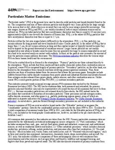
Figure 1-1 taken from the same white paper, shows the impact of small biases over a range of utility boiler capacities. Clearly, the larger the unit, the more impact small biases have on the resultant mass emission rate. Regulatory Drivers for fPM Method Improvement The recently promulgated MATS rule regulates power generating units at both major and area sources. The mercury and air toxics standards will affect Electric Generating Units (EGUs) that burn coal or oil for the purpose of generating electricity for sale and distribution through the national electric grid to the public. These include investor-owned units as well as units owned by the Federal government, municipalities, and cooperatives that provide electricity for commercial, industrial, and residential uses. The final rule identifies two subcategories of coal-fired EGUs, four subcategories of oil-fired EGUs, and a subcategory for units that combust gasified coal or solid oil (integrated gasification combined cycle (IGCC) units) based on the design, utilization, and/or location of the various types of boilers at different power plants. The rule includes emission standards and/or other requirements for each subcategory.

10061786

1-2

Figure 1-1 Effect of Particulate Measurement Bias on Mass Emission Rates

10061786

1-3

For all existing and new coal-fired EGUs, the rule establishes numerical emission limits for mercury, fPM (a surrogate for toxic non-mercury metals), and HCl (a surrogate for all toxic acid gases). The MATS rule fPM emission limits are summarized below in Table 1-1. The EPA estimates that there are approximately 1,400 units affected by the MATS rule, approximately 1,100 existing coal-fired units and 300 oil-fired units at about 600 power plants. The MATS compliance deadline for existing units is April 16, 2015. Table 1-1 Summary of MATS Rule fPM Emission Limits for New and Existing Units Subcategory

fPM (lb/MWh)

fPM (lb/MMBtu)

fPM (mg/dscm)

Existing – Not Low Rank Virgin Coal

0.3

0.03d

49.1a

Existing – Low Rank Virgin Coal

0.3

0.03d

48.7b

Existing IGCC

0.3

0.04e

65.5a

Existing - solid oil-derived

0.08

0.008d

14.0c

New – Not Low Rank Virgin Coal

0.09

0.009d

14.7a

New – Low Rank Virgin Coal

0.09

0.009d

14.6b

0.07f

0.007d

11.5a

0.09g

0.009d

14.7a

New – solid oil-derived

0.03

0.003d

5.2c

New – liquid oil continental

0.3

0.03d

52.3c

New – liquid oil non-continental

0.2

0.02d

34.9c

New IGCC

Notes: a Converted to concentration using F-factor of 9,780 dscf/106 (bituminous coal). b Converted to concentration using F-factor of 9,860 dscf/106 (lignite coal). c Converted to concentration using F-factor of 9,190 dscf/106 (oil). d Converted to lb/MMBtu using heat rate of 10,000 Btu/kWh. e Converted to lb/MMBtu using heat rate of 8,425 Btu/kWh. f Duct burners utilizing syngas. g Duct burners utilizing natural gas. lb/MWh = pounds pollutant per megawatt-electric output (gross). lb/MMBtu = pounds pollutant per million British thermal unit fuel input.

There are no federally mandated fPM emission limits for natural gas-fired combustion turbines in the U.S. However, natural gas combustion turbines are subject to a variety of air quality regulations deriving from the requirements for regions to meet National Ambient Air Quality Standards (NAAQS) for criteria pollutants, including fPM and PM2.5. Most fPM permit limits for gas turbines are established by State regulatory agencies, and are based on AP-42 emission factors. Table 1-2 shows the AP-42 fPM emission factors for natural gas and landfill gas-fired stationary combustion turbines.

10061786

1-4

Table 1-2 Summary of fPM AP-42 Emission Factors for Gas Turbines 1

Subcategory

fPM (lb/Mwh)

fPM (lb/MMBtu)

fPM (mg/dscm)

Natural Gas-Fired Turbines

2.2 x 10-2

0.0019a

3.5c

Landfill Gas-Fired Turbines

2.8 x 10-1

0.023b

39.2d

Notes: 1

Table 3.1-2a of AP-42 Emission Factors a Heat Rate for natural gas-fired combustion turbine, 11,569 Btu/kWh. b Heat Rate for landfill gas-fired combustion turbine, 12,200 Btu/kWh. c Converted to concentration using F-factor of 8,710 dscf/106 (natural gas). d Converted to concentration using F-factor of 9,391 dscf/106 (landfill gas).

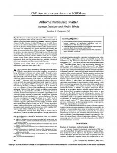
EPA Reference Methods for Filterable Particulate Matter (fPM) The principal EPA Reference Methods for filterable particulate testing from stationary sources are Methods 5, 17, and 201A. Diagrams of each of these methods, along with flow charts of the required method procedures are presented in Appendix A. There are also variations of some of these methods (e.g., Method 5B). All of the methods are derived from Method 5 and therefore the focus of this report will be on that method. Issues specific to Method 17 and Method 201A will be discussed when relevant. All of these methods are found in the Code of Federal Regulations (CFR) at 40 CFR 60 Appendix A. EPA maintains a web site with copies all of the current reference methods at http://www.epa.gov/ttn/emc/tmethods.html. Method 5 Method 5 is the base EPA Reference Method for measuring fPM from stationary sources. Figure 1-2 below shows a schematic of the Method 5 sampling apparatus or “sampling train”. The method uses a heated, out-of-stack filter, and therefore is applicable to both dry and wet stacks.

10061786

1-5

Figure 1-2 EPA Method 5 Sampling Apparatus

The sampling train consists of a sampling nozzle, a heated probe, a heated filter holder with a glass mat or quartz fiber filter, a series of impingers to cool the gas and collect water and other condensable material and a metering system to measure the volume of gas sampled. In addition, a pitot tube and manometer are used to determine stack gas velocity. The fPM is withdrawn through the nozzle and probe at the same velocity the gas is moving through the stack. This is known as isokinetic sampling. Method 5 makes use of several other EPA reference methods: • • • •

Method 1 for selection of sampling location and sampling points Method 2 (or its variants) for measuring stack gas flow rate Method 3 (or its variants) for determining the molecular weight of the stack gas Method 4 for determining the moisture content of the stack gas

10061786

1-6

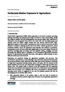
The heated sample probe and filter are intended to regulate the temperature of the stack gas to 248 ± 25 °F (120 ± 14 °C). This serves two purposes: 1. This temperature is sufficient to preclude the condensation and collection of water prior to the impingers, and 2. Adjusting the stack gas to a consistent temperature improves comparability of filterable and condensable particulate emissions across sources with a wide range of stack gas temperatures. In some variations of Method 5 (e.g., 5B and 5F) the probe and filter temperature are increased to 320 ± 25 °F (160 ± 14 °C) to minimize the collection of sulfuric acid. During the test, the sampling probe is moved from point to point within the stack. The sampling rate is adjusted at each point to match the stack gas flow rate at that point. At the conclusion of the test, the filter is recovered from the filter holder and the sample probe and nozzle are thoroughly rinsed and brushed to remove any particulate that may not have made it to the filter. The filter and rinses are sent to a laboratory where they are dried and weighed to determine total fPM collected. Method 17 Method 17 is similar to Method 5, except that it uses an in-stack filter rather than the heated filter used in Method 5. As a result, the particulate is collected at the temperature of the stack gas rather than at a “standard” temperature as in Method 5. The Method 17 sampling train is shown in Figure 1-3. Method 17 is generally not used for compliance testing. It is used primarily for performance tests (e.g., ESP efficiency) or diagnostic testing (e.g., fly ash LOI). Method 17 and Method 5 test results are not necessarily comparable. If the stack gas is cooler than the Method 5 standard temperature, the particulate collected on the in-stack filter may be greater than with Method 5, since additional material may condense on the filter at lower temperatures. Conversely, if the stack gas is warmer than the Method 5 standard temperature, the collected filterable particulate may be lower than with Method 5 since additional condensable material may have volatilized at the higher temperature and passed through the filter to the impingers. According to the method (Section 1.2)… “This method is applicable for the determination of PM emissions, where PM concentrations are known to be independent of temperature over the normal range of temperatures characteristic of emissions from a specified source category.” In addition to the above restrictions, the method may not be used in saturated gas streams or in gas streams with liquid droplets. The advantage of Method 17 over Method 5 is that in those limited circumstances where use of the Method 17 is allowed, the sampling train is simpler.

10061786

1-7

Figure 1-3 EPA Method 17 Sampling Apparatus

Method 201A Method 201A is similar to Method 17 in that it uses an in-stack filter. However, in the case of Method 201A, the filter is preceded by a pair of cyclones with different cut sizes. The net result is that the particulate captured by the Method 201A train is partitioned into three particle size fractions: First Cyclone: Removes fPM greater than 10 microns Second Cyclone: Removes fPM greater than 2.5 microns. Therefore, the catch from the second cyclone is fPM between 10 and 2.5 microns. • Filter: Captures remaining filterable particulate less than 2.5 microns. The combined catch of Cyclone 2 and the filter is PM10. • •

10061786

1-8

Method 201A (shown in Figure 1-4) differs from Method 5 and Method 17 in one important respect – isokinetic sampling is not used. Since the two cyclones require a constant velocity to achieve their designed particulate size cut-points, the sampling rate is not adjusted for every sampling point as it is for Methods 5 and 17. Instead, an average sampling rate is estimated for the entire test and remains constant at each point.

Figure 1-4 EPA Method 201A Sampling Apparatus

This method cannot be used in stacks with liquid water droplets present, and there is currently no EPA-approved method for measuring PM2.5 in a wet stack. Thus, units with wet stacks that are required to test for PM2.5 must use Method 5, which will generally overestimate PM2.5 emissions.

10061786

1-9

Overview of fPM Concentration and Mass Emissions Determination Results from a particulate stack test may be expressed in two ways: 1. As a concentration – gr/dscf or mg/dscm 2. As a mass emission rate – lb/hr, lb/mmBtu, kg/GJ, lb/MW Since most recent EPA rules, including MATS, establish mass emission limits for affected sources, the focus of this report is on mass emissions rather than concentration. However, all of the concepts discussed apply equally to concentration units. In the broadest sense, mass emissions (lb/hr) are determined by combining three other measured parameters as shown in Figure 1-5.

Figure 1-5 Determination of Mass Emissions (lb/hr)

These four parameters are related by Equation 1-1: Eq. 1-1

Where: E lb/hr = mass emission rate (lb/hr) m n = mass of particulate collected (mg) Q std = volumetric flow of the stack gas (dscfm) k

= conversion constant (0.1323 for the units used here)

Method Performance Terminology This report focuses on the performance of fPM methods, particularly at low emissions levels. In discussing method performance it is important to define our terminology, as many of the common metrics are subject to considerable confusion. Some of the most important terms that are often used to describe method performance are defined here, to provide a basis for subsequent discussion. A more detailed discussion of each of these terms is provided in Appendix B.

10061786

1-10

Accuracy, Precision, and Bias When evaluating test methods or measurement equipment, one often encounters the term “accuracy.” Often, numbers or ranges are associated with the term. For example a specification may state that a particular instrument is accurate to within ±2%. What exactly does this mean? The term “accuracy” has no generally agreed-upon scientific meaning. In a broad sense, it refers to “closeness to truth.” Accuracy is a qualitative concept often used in marketing literature to imply reliable measurement. The National Institute of Standards and Technology (NIST) makes this statement this regarding accuracy [NIST, 1994]: “Since accuracy is a qualitative concept, one should not use it quantitatively, that is, associate numbers with it...” When a vendor lists an instrument specification for “accuracy” the user has no idea what is meant absent a specific explanation in the specification. Often in instrument specifications, the term “accuracy” is used to mean precision or repeatability. Sometimes “accuracy” means bias. At other times, it is used as a reference to a linear regression correlation coefficient for a calibration curve. And sometimes it is just an engineering estimate not based on any measured values. In this report, we shall avoid any use of the term “accuracy.” Instead, we will use the terms “precision” and “bias” to refer to random and systematic errors. This not only prevents confusion but also is consistent with national standards on reporting uncertainty from ASTM, NIST, and others. These terms as used in this report conform to the definitions provided in ASTM E177 “Standard Practice for Use of the Terms Precision and Bias in ASTM Test Methods”. The term “precision” refers to the repeatability of a measurement. If a measurement is taken several times and the results are all clustered closely together, the method is said to be “precise” for that application. The general term “uncertainty”, used frequently in this report, also refers to repeatability. The precision of a test method may be evaluated in two ways -- as repeatability and as reproducibility. If method precision is determined using repeated measurements with the same equipment and operator for all repetitions (as is typical in a stack test or RATA), it is often referred to as “repeatability.” The second way in which method precision may be evaluated is to compare repeated measurements under one set of conditions to repeated measurements under a different set of conditions. When precision is evaluated in this way, it is referred to as “reproducibility.” The term “bias” refers to how far a measurement is from the “true” value of the measured parameter. In all cases, the “true” value is unknown so a generally accepted standard (e.g., calibration gas, check weight, or calibrated standard pitot) is used as a comparison. When referring generally to the concept of “closeness to truth,” this report uses the term “reliable” rather than “accurate”, to avoid the issues discussed above. In the absence of bias, the “true” value of the measured parameter is estimated by the mean of the sample data. The more sample data used to calculate the mean, the closer it will be to the true, unknown value. The number of data points needed to estimate the true value depends on the

10061786

1-11

magnitude of random error “noise” and the level of confidence required in the final result. In effect, the true value is estimated by the average of the noise. When systematic error (bias) is present in a measurement process, the data are shifted away from the true value and so the average will not provide a reliable estimate. Bias factors should be eliminated from a measurement process whenever possible. If not possible, then the effects should be minimized. If the magnitude of a bias is known, the data may be corrected to compensate for the bias effects (assuming relevant regulations do not prohibit this). Quantifying Uncertainty: What Does ± Mean? One often sees a measured value such as a flow rate or mass emission rate written in the form: Eq. 1-2

Where X is the average value of several measurements and u is an uncertainty or error term. What exactly does this mean? Consider an example: the fPM concentration in a stack is measured over five test runs. The results are shown in Table 1-3: Table 1-3 Example fPM Stack Concentrations Over Five Runs Run

1

2

3

4

5

Average

Result (mg/dscm)

50

52

48

51

49

50

The results in X ± u form may be stated correctly as any of the following (as well as in other ways not listed here), as shown in Table 1-4: Table 1-4 Uncertainty Expressed in Various Ways X±u

Description

50 ± 2 mg/dscm

Average ± Half Range

50 ± 0.71 mg/dscm

Average ± Standard Error of the Mean

50 ± 1.58 mg/dscm

Average ± One standard deviation

50 ± 3.16 mg/dscm

Average ± Two standard deviations

50 ± 1.96 mg/dscm

Average ± 95% confidence interval of the mean

50 ± 3.26 mg/dscm

Average ± 99% confidence interval of the mean

50 ± 3.16%

Average ± Relative standard deviation

50 ± 3.93%

Average + Relative 95% confidence interval

If any of these results were listed in a report or study without further explanation, the reader would not know which of these many approaches was used to calculate u. In this report, the uncertainty term, u, will sometimes be presented alone and sometimes in the form X ± u. In either case, to avoid confusion, the u will always refer to one standard deviation of the mean, unless specifically declared as something different. If u is expressed as a percent, it

10061786

1-12

will always represent the relative standard deviation (RSD) – the standard deviation divided by the average of the data. The standard deviation is a descriptive statistic, that is, it describes the spread of the underlying data from which it was calculated, i.e., that particular set of test data. The extent to which it is informative about future data collected with the test method depends on many factors including how many data points were used to calculate the standard deviation, how representative that data was, and whether the conditions under which future data are collected have changed. In fact, due to the relatively small size of the example data used above (5 runs), the calculated standard deviation most likely under-estimates the true variability of the test method. To correct this effect another statistic, the t-statistic, is used. A full discussion of this is beyond the scope of this report. However, given a large enough sample size, with representative, normally-distributed data, and conducting future tests under essentially identical conditions, the standard deviation may estimate future data spread as follows: •

About 67% of data will fall within ±1 standard deviation of the value.

•

About 95% of data will fall within ±2 standard deviations of the value.

•

About 99.7% of data will fall within ±3 standard deviations of the value.

It may be tempting to assume that these ± expressions imply that the true value of the measured parameter (flow, concentration, etc.) lies within the range of X-u to X+u. However, that may not be the case. The uncertainty term, u, is a measure of precision (repeatability). It does not take into account any bias present in the measurement process. The true value of any measured parameter is unknowable. We make the assumption that if our measurement process is free of bias, then the average of repeated measurements will approach the true value the more measurements we take. However, no measurement system is completely bias-free. In fact, in many cases, the measurement bias may be significant and the magnitude of bias may be unknown. If significant bias exists in the measurement process, the “true” value could very well lie outside the specified range. For example, assume the “true” value of fPM concentration in the example above is 50 mg/dscm. However, in this case, assume the testing company uses a contaminated reagent when recovering the sample that adds 5 mg/dscm of bias to the results from each run. The average measured value is now 55 ± 1.58 mg/dscm – a range of about 53.4 to about 56.6. In this case, the true value, 50 mg/dscm, lies outside the specified error range. Even using a 99% confidence interval of ±3.26 mg/dscm, the true value is outside the specified range. In all cases, an uncertainty range of ±u assumes the absence of any significant bias in the measurement process. However, as this report will discuss later, bias is often the largest source of error in a filterable particulate test result. Discussion of Detection and Quantitation Limits for fPM Methods The concept of a detection limit, sometimes called the Limit of Detection (LOD), is one of the most controversial in all of metrology. It has undergone much change over the past 40 years and is still an unsettled issue.

10061786

1-13

Conceptually, the detection limit is the minimum amount or concentration of a substance that must be present for a measurement process to distinguish it from a sample that does not contain the substance, with a given degree of confidence. In practice, the measured substance may be present in the measurement system itself. For example, in a gravimetric (mass-based) method such as EPA Method 5, variations in the filter weight may contribute some mass. Thus, the detection limit is defined as the minimum amount that can be distinguished from background. Most EPA reference methods specify detection or “sensitivity” limits derived from initial validation tests conducted under a limited range of conditions. For EPA stack test methods, those conditions included stack gas concentrations several orders of magnitude higher than the current emission limits. Also problematic is that the stated limits are often calculated from “analytical” detection limits, i.e., they are based solely on the laboratory analysis portion of the method. A typical laboratory method involves a single measurement using an instrument with a single sensor or detector. As the concentration of the analyte decreases, the signal resulting from the presence of the analyte becomes harder and harder to distinguish from detector noise. Another way to say this is that the relative standard deviation of a method tends to increase geometrically as it approaches the detection limit, a pattern known in environmental statistics as the Horwitz curve [Horwitz, 1980]. A stack test method, however, involves multiple measurements with multiple sensors – some in the field and some in the laboratory. Each of these measurements contributes to the overall uncertainty of the final result. The uncertainty of the analytical portion of the method is often far lower than the uncertainty for the field contributors. This is discussed in more detail later in this report. A related concept is the “limit of quantitation” or LOQ. When applied to a stack test, the LOQ is also sometimes called the ‘practical quantitation limit” or PQL. The LOQ is established at a level where the data signal is presumed high enough above “noise” to achieve acceptable precision. Typically (and somewhat arbitrarily), the LOQ is often set at about three times the detection limit or 9-10 times the standard deviation of the blank measurements. The EPA has defined an analytical detection limit for gravimetric analysis of 0.5 mg per weighing. For Method 5, EPA states that the Method Detection Limit (MDL) is 1 mg and the PQL is 3 mg [EPA, 1999]. Because of the difficulty of relating a gravimetric detection limit to an in-stack detection limit, and the fact that precision is only one component of method performance (bias is the other) this report takes a different approach to evaluating the lowest limit at which fPM methods can be used to provide reliable data. Rather than attempting to identify an “in-stack quantitation limit” – i.e., a discrete emission rate at which a fPM method will provide reliable data on a specific source type with a reasonable sampling duration, the report discusses the factors that have the greatest impact on method uncertainty and recommends concrete measures that can be taken to improve performance. Some of these measures will have the effect of lowering the gravimetric detection limit, but they must be combined with other measures to minimize bias and tighten method specifications before they result in better performance at low emission levels.

10061786

1-14

2

EVALUATING TEST METHOD UNCERTAINTY One important piece of information needed to evaluate the applicability of a method at low emission levels is the precision or uncertainty of the method under those conditions. There are two approaches to conducting this uncertainty analysis – top down and bottom up. Each of these approaches is discussed below, along with results from studies of fPM methods using each approach. Top Down Analysis The top down approach utilizes replicate measurements to obtain information on method performance. This is generally the best way to characterize the uncertainty and reliability of a test method. Multiple, simultaneous tests are conducted with several sampling trains, positioned as close to each other in the stack as possible. One can then compare the data to see how much test-to-test variation is present. The assumption made in these multi-train studies is that the primary source of variability in the results between sampling trains is the test method: depending on the stack gas flow characteristics, that assumption may or may not be valid. An additional enhancement to a top down study is to use different testing companies and personnel for each sampling train. These “collaborative” studies allow measurement of the additional measurement variation introduced by different testers and test companies. That information can be important in assessing method reliability and bias across multiple sites and sampling episodes. Top Down Studies of Method 5 Several top down studies of Method 5 have been conducted at different combustion sources. No top down studies were identified for Method 17 or Method 201A. In the early1970’s, Hamil [1974; 1976] conducted a series of collaborative studies for the U. S. EPA to determine method precision and bias of Method 5. These studies were conducted on a power plant, two municipal waste combustors and a portland cement plant. Rigo [1999] published a collaborative study (along with several other methods), also conducted at a municipal waste combustor. Paired or quad sampling trains were used in these studies: two or four sample probes were placed close to one another in the stack and each was connected to a separate sampling train. The advantage of using these paired or quad trains is that replicate measurements can be made which can then be used to estimate method precision independently of process variation. Depending on the study, sometimes a single individual operated all of the trains and sometimes each train was operated by a separate individual, often from another testing organization. Figure 2-1 shows the range of particulate concentrations observed in each study as well as the range of relative standard deviations across all test runs. Stack gas concentrations corresponding to the emission limits from the MATS rule for existing and new/reconstructed coal-fired units are shown for comparison.

10061786

2-1

Note that the MATS emission limits for existing coal-fired units fall within the ranges covered by Rigo and Hamil and the fPM results are shown to have a relative standard deviation of less than 10% at these concentrations. The Hamil 2 tests were two hours in duration. The Rigo tests were four hours in duration. The MATS limits for new/reconstructed coal units and several other source categories, fall below the range of concentrations evaluated in these historical studies. In addition, since the test duration in these studies spanned multiple hours, fPM catches were large, in some cases greater than 100 mg. Thus, the historical studies are of limited use in assessing the performance of the method at concentrations at or below those limits and particularly at lower fPM catches. The results of the Hamil 3 tests [Hamil, 1976] show both the promise and the problem with Method 5. While the particulate concentrations found in the study are higher than those typically encountered today, this data set is the most robust, with 8 simultaneous measurements. Figure 2-2 shows the percent deviations of the Hamil 3 results for each run from the average for each of the eight test teams/laboratories, relative to the average run concentration. The deviations were calculated as shown in Equation 2-1. Eq. 2-1

The best performing test team, Lab 106, is shown by the blue line. This team demonstrated consistent results within 5% of the run average for all of the runs except Run 12, which had a deviation of 10%. The results from Lab 106 give an indication of the capability of Method 5 to produce reliable data. These were simultaneous runs taken with four sets of paired sampling trains. The spread in the data for each run gives an indication of the variability that may be expected from testing firm to testing firm. However, it should be noted that in 1976, Method 5 was fairly new and test teams may not have had much experience with the method at that point in time. Figure 2-3 and Figure 2-4 show the run-by-run deviations from the Hamil 2 [1976] and Rigo [1999] studies. In these two studies, the fPM concentrations encompassed the limits required by the MATS rule for existing coal-fired power plants. In the Hamil 2 study, Lab B achieved results of about ±5% of the run average. This is the same “best performance” laboratory as in Hamil 3. In the Rigo study, there were only two sampling trains, so the deviations are symmetrical around zero and neither train can be considered as “best”. Note that in both studies, the range of deviations tends to be approximately ±10% of the run average.

10061786

2-2

Figure 2-1 Particulate Concentration vs. Relative Standard Deviations of fPM in Historical Studies

10061786

2-3

Figure 2-2 EPA Method 5 Collaborative Study Results (Hamil 3 Data)

10061786

2-4

Figure 2-3 EPA Method 5 Collaborative Study (Hamil 2 Data)

10061786

2-5

Figure 2-4 EPA Method 5 Collaborative Study (Rigo, 1999 Data)

10061786

2-6

Shigehara used data from Hamil and Rigo as well as others to compile a succinct summary of the precision of various EPA test methods including Methods 1-5 [Shigehara 1993]. ASME conducted a statistical re-analysis of the Hamil and Rigo data for Phase 1 of their ReMAP project [ASME 2001]. Table 2-1 summarizes the Method 5 precision estimates and concentration ranges from each of the historical studies and re-analyses. Table 2-1 Summary of EPA Method 5 Precision Estimates Source

RSD

Conditions

Source

Hamil 1 [1974]

8.8% - 20.5% (@ 141-240 mg/dscm)

Reproducibility

PP

Hamil 2 [1974]

1.4% - 10.4% (@ 49-64 mg/dscm)

Reproducibility

MWC

Hamil 3 [1976]

7.1% - 18.5% (@ 82-255 mg/dscm)

Combination

MWC

Shigehara [1993]1

10.4% (@ 133 mg/dscm)

Repeatability

MWC

Rigo [1997]

0.1% - 9.6% (@ 15-70 mg/dscm)

Repeatability

MWC

ReMAP [2001]2

4.8%-12.2% (@ 15-240 mg/dscm)

Combination

PP/MWC

1

Re-analysis of a portion of the Hamil 3 data Combined analysis of Hamil 1, 2, 3 and Rigo PP – power plant; MWC – municipal waste combustor

2

The following quotation from the ReMAP report illustrates the difficulty in coming to any definitive conclusion from such a diverse set of studies. “…it is difficult to draw firm conclusions about the actual precision of Method 5. However…it appears that Method 5 standard deviation varies approximately linearly with concentration and that the relative standard deviation for the method is approximately constant. For fPM concentrations between 15 and 217 mg, the best estimate for the relative standard deviation for Method 5 is between about 4.8% and 12.2%.” Shigehara also conducted additional tests to characterize the detection limit of Method 5 [Shigehara 1996]. The study focuses only on the analytical portion of the method – weighing filters and rinses. In this report, Shigehara concludes that a minimum of 3.6 mg of particulate is needed to achieve a relative standard deviation of 10% in the analytical result. However, to achieve this precision he used a modified Method 5 weighing process weighing both the filter and rinse containers together. Benefits and Limitations of the Top Down Approach Collaborative studies and other “top down” approaches provide the best estimates of method performance in the field. Actual test data is used for the analysis and all potential sources of variability present at that time for the source and conditions, whether known or unknown, are expressed in the final result. As noted earlier, the precision determination will incorporate both

10061786

2-7

measurement variability and source variability, which is generally assumed to be negligible when sampling trains are collocated. In some instances, this assumption may not be valid, however. However, a top down analysis is expensive to conduct, particularly in collaborative studies with multiple testing organizations involved. In the 40 years that Method 5 has been in existence, only four collaborative studies have been identified – three of which were conducted in the 1970’s. Furthermore, top down analyses are limited by the specific data collected and so may be limited in their applicability. In the case of Method 5 for example, none of the four collaborative tests included conditions with a filter catch less than about 15 mg (estimated). These tests are of limited value in characterizing method performance as the filter catch approaches zero. Bottom Up Analysis In a bottom up analysis, the uncertainty of each individual measurement contributing to the final emission concentration or rate is determined and then combined or “propagated” to determine the uncertainty of the final mass emission value. A mass emission rate requires many individual measurements – pressure, temperature, mass, concentration, etc. Each individual measurement has its own associated uncertainty. For example, one gravimetric laboratory reports a standard deviation for repeated weighings of a blank filter of about 0.03 mg. This translates to a relative standard deviation for a typical filter weight of about 0.008%. Method 5 requires multiple weighings of filters (tare, sample, blank) and probe rinses – each contributes to the overall uncertainty of the method. Bottom Up Analysis of Method 5 for a Coal-Fired Boiler A bottom up analysis of Method 5 was conducted, examining two cases [Clean Air Engineering, 2012]. 1. A 595 MW utility boiler firing Powder River Basin coal 2. A gas-fired industrial boiler The utility boiler case is presented in this section. Details of both cases, including the equations, methodology, and sources of measurement uncertainty values, are presented in Appendix C. As discussed in Section 1, there are three component parameters contributing to the calculation of the lb/hr mass emission rate: 1. The volume of gas sampled (Vmstd) 2. The volumetric flow rate of the stack gas (Qstd) 3. The total particulate mass collected (mn) Each of these parameters is determined by a combination of direct measurements and calculations, as described below. Volume of Gas Sampled (V mstd ) V mstd, the volume of gas pulled through the meter box, is one of the three parameters used to calculate the lb/hr mass emission rate. Figure 2-5 shows the input parameters to V mstd and how they are related.

10061786

2-8

Figure 2-5 Input Parameters for V mstd

Parameters that are directly measured are shown in tan. Parameters calculated from these measurements are shown in green. Table 2-2 lists all directly measured parameters used to calculate V mstd . The sample data from the utility boiler case is presented along with the estimated measurement uncertainty (± SD) for each measurement. Depending on the parameter, the measurement uncertainty was obtained from uncertainty studies (e.g., Shigehara, 1993), from instrument vendor specifications, or from actual laboratory studies. Table 2-2 Directly Measured Parameters Used in V mstd Calculation Measured Parameter (direct measurements)

Unit

Sample Data

Measurement Uncertainty (Std. Dev.)

Barometric Pressure (P bar )

in. Hg

29.21

0.0107

Meter Correction Factor (Y d )

unitless

1.002

0.0122

Volume of Sample Gas Metered Final (V mf )

dcf

63.321

0.0020

Volume of Sample Gas Metered Initial (V mi )

dcf

23.175

0.0020

Meter Orifice Pressure Differential (∆H)

in H 2 O

Multiple

0.0408

Meter Temperature (T m )

°F

Multiple

0.58

10061786

2-9

Table 2-3 lists intermediate values calculated from the direct measurements above. The individual measurement uncertainties are propagated into each calculated result according to standard statistical practice for error propagation, as described in Appendix C. Table 2-3 Intermediate Values Used in V mstd Calculation Calculated Parameter (calculated from the measurements above)

Unit

Sample Data

Propagated Uncertainty (st. dev)

Meter Absolute Pressure (P meter )

in. Hg

29.30

0.0422

Volume of Sample Gas Metered (V m )

dcf

40.15

0.0029

Average Meter Orifice Pressure Diff. (∆H)

in H 2 O

1.212

0.0408

Average Meter Temperature (T m )

°F

56.5

0.58

Finally, the intermediate values are combined to calculate the volume of gas sampled. As above, the individual uncertainties from the component parameters are propagated into the final result, as shown in Table 2-4. Table 2-4 Final Result Calculations for V mstd Final Calculated Result (calculated from all of the above)

Unit

Sample Data

Propagated Uncertainty (st. dev)

Volume of Gas Sampled (V mstd )

dscf

40.25

0.6437

The final result for Volume of Gas Sampled is 40.25 ± 0.64 dscf. This result may also be expressed as ±1.6% RSD or as ±3.2% as a 95% confidence interval. Volumetric Flow Rate of the Stack Gas (Q std ) Q std , the volumetric flow rate of the stack gas (volume of gas per unit of time), is the second of the three parameters used to calculate the lb/hr mass emission rate. Figure 2-6 shows the input parameters to Q std and how they are related. Parameters that are directly measured are shown in tan. Parameters calculated from these measurements are shown in green.

10061786

2-10

Figure 2-6 Input Parameters for Q std

10061786

2-11

Table 2-5 lists all directly measured parameters used to calculate Q std . For more details on calculations and sources of uncertainty estimates, see Appendix C. Table 2-5 Directly Measured Parameters Used to Calculate Q std Measured Parameter (direct measurements)

Unit

Sample Data

Measurement Uncertainty (st. dev)

O 2 Concentration (O 2 )

%

13.5

0.11

CO 2 Concentration (CO 2 )

%

7.0

0.11

Velocity Head Pressure Differential (∆p)

in H 2 O

1.068

0.0041

Stack Temperature (T s )

°F

Multiple

0.58

Barometric Pressure (P bar )

in. Hg

29.21

0.0107

Sample Gas Static Pressure (P g )

in H 2 O

-1.0

0.2041

Stack Diameter (D s )

inches

319.0

0.0255

Pitot Tube Coefficient (C p )

unitless

0.84

0.0019

Moisture Fraction

unitless

0.152

0.0028

Table 2-6 lists parameters calculated from the direct measurements presented above. The individual measurement uncertainties are propagated into each calculated result according to standard statistical practice for error propagation. Table 2-6 Intermediate Values Used in Q std Calculation Calculated Parameter (calculated from the measurements above)

Unit

Sample Data

Propagated Uncertainty (st. dev)

Stack Area (A s )

sq. ft.

555.01

0.0888

Average Stack Temperature (T s )

°F

129.3

0.58

Average Square Root of ∆p (√∆P)

√in. H 2 O

1.049

0.0041

Molecular Weight Dry Basis (M d )

lb/lb-mol

30.44

0.1556

Dry Molecular Weight x Moisture Term (ω)

lb/lb-mol

4.63

0.0885

Molecular Weight Wet Basis (M s )

lb/lb-mol

28.55

0.1790

Sample Gas Absolute Pressure (P s )

in. Hg

29.14

0.2044

Ideal Gas Law Term (φ)

See Note 1

0.71

0.0074

Velocity of the Stack Gas (Vs)

ft/sec

63.40

0.3801

Pitot Tube Coefficient (C p )

unitless

0.84

0.0019

Moisture Fraction

unitless

0.152

0.0028

Note 1: (φ, √((°R)/((lb/lbmol)∙(in. Hg))))

10061786

2-12

Finally, the intermediate calculated results are combined to calculate the volumetric flow rate of the stack gas. The results are shown in Table 2-7. As above, the individual uncertainties from the component parameters are propagated into the final result. Table 2-7 Final Result Calculations for V mstd Final Calculated Result (calculated from all of the above)

Unit

Sample Data

Propagated Uncertainty (st. dev)

Volumetric Flow Rate of the Stack Gas (Q std )

dscfm

1,562,217

32,941

The final result for Stack Gas Volumetric Flow Rate is 1,562,217 ± 32,941 dscfm, rounded to 1,562,000 ± 33,000. This result also may be expressed as ±2.1% RSD or ±4.2% as a 95% confidence interval. Total Particulate Mass Collected (m n ) The third parameter used to calculate the lb/hr mass emission rate is m n , the total mass of the fPM collected from the filter and the rinse. Figure 2-7 shows the input parameters to m n and how they are related. Parameters that are directly measured are shown in tan. Parameters calculated from these measurements are shown in green.

Figure 2-7 Input Parameters for m n

10061786

2-13

Table 2-8 lists all directly measured parameters used to calculate m n . Table 2-8 Directly Measured Parameters Used to Calculate m n Measured Parameter (direct measurements)

Unit

Sample Data

Measurement Uncertainty (st. dev)

Filter Mass Initial (m fi )

g

0.3689

0.00003

Filter Mass Final (m ff )

g

0.3754

0.00003

Solvent Mass Initial (m si )

g

4.9737

0.00003

Solvent Mass Final (m sf )

g

4.9833

0.00003

Blank Mass Initial (m bi )

g

4.9207

0.00003

Blank Mass Final (m bf )

g

4.9210

0.00003

Volume of Solvent Rinse (V s )

ml

52

0.07

Volume of Solvent Blank (V b )

ml

50

0.07

Table 2-9 lists intermediate values calculated from the direct measurements above. The individual measurement uncertainties are propagated into each calculated result according to standard statistical practice for error propagation. Table 2-9 Intermediate Values Used in m n Calculation Calculated Parameter (calculated from the measurements above)

Unit

Sample Data

Propagated Uncertainty (st. dev)

Filter Mass (m f )

g

0.00650

0.000042

Solvent Mass (m s )

g

0.00960

0.000042

Blank Mass (m b )

g

0.00031

0.000042

Finally, the intermediate calculated results are combined to calculate the total sample mass as shown in Table 2-10. As above, the individual uncertainties from the component parameters are propagated into the final result. Table 2-10 Final Result Calculations for m n Final Calculated Result (calculated from all of the above)

Unit

Sample Data

Propagated Uncertainty (st. dev)

Total Particulate Mass Collected (m n )

g

0.01579

0.000060

The final result for Total Particulate Mass Collected is 0.01579 ± 0.00006 g. This result may be expressed as ±0.4% RSD or ±0.8% as a 95% confidence interval.

10061786

2-14

Mass Emissions (lb/hr) The results from the three component parameters are combined to determine the final mass emission rate, shown in Table 2-11. The final calculated uncertainty for the mass emission rate is shown in Table 2-12. Table 2-11 Three Components for Final Mass Emission Rate Calculated Parameter (from the final calculated results above)

Unit

Sample Data

Propagated Uncertainty (st. dev)

Volume of Gas Sampled (V mstd )

dscf

40.25

0.6437

Volumetric Flow Rate of the Stack Gas (Q std )

dscfm

1,562,217

32,941

Total Particulate Mass Collected (m n )

g

0.01579

0.000060

Unit

Sample Data

Propagated Uncertainty (st. dev)

lb/hr

81.07

2.17

lb/MMBtu

0.0162

0.0004

Table 2-12 Final Calculated Results for Mass Emission Rate

Final Calculated Result Mass Emission Rate (E lb/hr ) Mass Emission Factor (E lb/MMBtu ) 1

1

Equivalent Emission Factor for a 500 MW PRB-fired unit having a nominal heat rate of 10,000 Btu/kWh.

The final mass emission rate from the bottom up analysis of the utility boiler case is 81.07 ± 2.2 lb/hr, or 0.0162 ± 0.0004 lb/MMBtu for a typical 500 MW PRB-fired unit. This may be expressed as an RSD of about ±2.7% or as a 95% confidence interval of about ±5.3%. This uncertainty estimate does not completely take into account differences between testing firms. Therefore, this estimate should be considered as a floor. A gas-fired utility case was also examined and yielded approximately the same RSD at a much lower concentration (0.00049 gr/dscf vs. 0.00605 gr/dscf). Benefits and Limitations of the Bottom Up Approach The major benefit to using the bottom up approach to uncertainty analysis is cost. Individual measurement uncertainties can often be obtained from equipment specification sheets, from previous studies, or directly by repeated measurements of a standard. An excellent source of uncertainties associated with common stack testing measurements is Shigehara [Shigehara, 1993; 1996]. This was the source for many of the measurement uncertainties used in the bottom up analysis. Another benefit of using the bottom up approach is that the uncertainty may be estimated for almost any desired condition. For example, none of the collaborative studies looked at low level particulate catches. They looked at stack gas with low fPM concentrations, but the tests were multiple hours in length. Rigo, for example, collected fPM in excess of 100 mg of particulate over a four hour test (estimated). These studies are therefore not particularly instructive in

10061786

2-15

determining the uncertainty of the methods when applied to low particulate catches. It is desirable to understand the uncertainty associated with lower particulate catches in order to reduce sampling time while still maintaining acceptable uncertainty in the final result. This can be accomplished with the bottom up analysis. The major limitation of the bottom up approach is that the end result is highly dependent on the assumptions made for each of the individual component measurements. Also, neglecting to include a significant source of uncertainty in the analysis will skew the final result. In general, a top down analysis conducted under conditions similar to the conditions of interest is always preferable to a bottom up analysis. However, if a top down analysis is not available, a carefully conducted bottom up analysis may provide insight. The results of a bottom up analysis should be considered as a lower bound of uncertainty given the potential for missing important uncertainty sources. Additional Insights from the Bottom Up Analysis When characterizing the performance of a test method, it is not correct to speak of “the” uncertainty of the method. Method uncertainty is not constant over all test conditions. As discussed above, one of the benefits of using a bottom up analysis is that it is possible to simulate a range of conditions over which uncertainty can be estimated. Like most test methods, absolute uncertainty (standard deviation) for Method 5 is directly proportional to the magnitude of the measured value. As the measured value increases, so does absolute uncertainty. Table 2-13 shows an example using the bottom up uncertainty model to estimate mass emissions from a coal-fired utility boiler. Table 2-13 Bottom Up Certainty Model Example fPM Mass (mg)

Mass Emissions (lb/hr)

Standard Deviation (lb/hr)

Relative Standard Deviation (%)

10

51.35

1.40

2.7%

20

102.69

2.74

2.7%

Note that while the absolute uncertainty increases with increased fPM mass, the relative uncertainty is virtually unchanged. This finding has been addressed in other studies. The ReMAP study, for example states: “…Method 5 standard deviation varies approximately linearly with concentration and…the relative standard deviation for the method is approximately constant.” [ReMAP 2001] The analysis in this report supports this finding over the range of concentrations included in the ReMAP study, i.e., from 15 to 217 mg. However, as emissions approach zero, relative uncertainty begins to increase exponentially. Table 2-14 shows additional model estimates from the same source with lower fPM mass collection assumptions.

10061786

2-16

Table 2-14 Additional Model Estimates fPM Mass (mg)

Mass Emissions (lb/hr)

Standard Deviation (lb/hr)

Relative Standard Deviation (%)

1

5.13

0.34

6.5%

3

15.40

0.51

3.3%

5

25.67

0.75

2.9%

10

51.35

1.40

2.7%

20

102.69

2.74

2.7%

This effect is shown graphically in Figure 2-8 and Figure 2-9. These graphs were calculated using the bottom up uncertainty model over a range of particulate mass loadings. The calculated curves for two cases, a coal-fired utility boiler and a gas-fired industrial boiler, show that these curves are consistent across a wide range of source parameters. The curves for fPM mass are identical, as one would expect since the analytical procedure is identical in both cases. In both cases, below approximately 1.3 mg the uncertainty of the final mass emission rate (lb/hr) exceeds ±10%. Below approximately 0.6 mg the uncertainty of the final mass emission rate (lb/hr) exceeds ±20%. Note that this finding contradicts the ReMAP [2001] study, which predicted improved method precision as fPM concentration approaches zero.

10061786

2-17

Figure 2-8 Relative Uncertainty as a Function of fPM Mass Collected

10061786

2-18

Figure 2-9 Relative Uncertainty as a Function of fPM Mass Collected (Low Masses)

10061786

2-19

Error Apportionment The apportionment of test measurement variability between sampling and analysis components is of interest when discussing the sensitivity of methods. Detection limits based on analytical measurements do not reflect the true capabilities of a method, as they ignore variability from sampling operations. The bottoms up uncertainty model can provide information on this topic. Of the three elements contributing to a fPM measurement, two are sampling related – V mstd and Q std – and one is analytical – m n . Each element contributes a share of uncertainty in the final result. Since these are the only elements contributing to the final result, the contribution of uncertainty from all three totals 100% of the uncertainty in the final mass emission rate. At relatively high fPM concentrations, the proportion that each element contributes to the final result is essentially fixed, as shown in Table 2-15. Table 2-15 Final Mass Contribution Uncertainty at High fPM Levels Vmstd

Qstd

mn

Uncertainty Source

Sampling

Sampling

Analytical

Contribution to Final Mass Emission Uncertainty

35%

63%

2%

Approximately 98% of the uncertainty in the lb/hr mass emission rate is attributable to sampling related parameters at high fPM levels. Analytical parameters contribute just 2% to the total error. This apportionment changes, however, as fPM concentrations approach zero. This is shown in Figure 2-10 and Figure 2-11. Above about 10 mg the uncertainty apportionment is approximately constant at the proportions shown in Table 1-4. At about 7 mg, the fPM mass measurement uncertainty apportionment increases to about 10% of the total. At 2-3 mg, the fPM mass uncertainty apportionment is approximately equal to the V mstd and Q std uncertainty. Below approximately 2 mg, the fPM mass uncertainty dominates. This analysis has significant implications for conducting Method 5 tests at low fPM concentrations, particularly when viewed in conjunction with the data presented in Figure 2-8. Figure 2-8 shows that below 2 mg of fPM mass, the relative uncertainty of the final lb/hr mass emission rate begins to rise exponentially. At roughly the same 2 mg fPM mass value, Figure 2-10 and Figure 2-11 show that most of the uncertainty is attributable to analytical sources rather than sampling sources. This strongly indicates that particular attention must be paid to the laboratory analysis of the fPM samples when performing Method 5 on low concentration sources. Of course an alternative would be to increase sampling time or sampling rate in order to increase the fPM mass collected.

10061786

2-20

Figure 2-10 Changes in Error Apportionment as a Function of fPM Mass – Area Plot

10061786

2-21

Figure 2-11 Changes in Error Apportionment as a Function of fPM Mass – Line Plot

10061786

2-22

Table 2-16 applies the findings of the uncertainty model to estimate how much fPM mass must be collected in order to achieve the desired confidence level of the final mass emission rate. For example, if the reported analytical detection limit is 0.3 mg and the confidence required in the final mass emission rate is 10% RSD, the minimum fPM mass that must be collected during the stack test is 2.0 mg. Table 2-16 Minimum fPM Mass Needed to Achieve Desired Confidence in Final Mass Emission Rate Reported Lab Detection Limit (mg)

Min. Mass (mg) Needed for ±10% @ 0.99 confidence

Min. Mass (mg) Needed for ±10% @ 0.95 confidence

Min. Mass (mg) Needed for 10% RSD

Formula

(DL*100)/3

(DL*50)/3

(DL*20)/3

0.15

5.0

2.5

1.0

0.18

6.0

3.0

1.2

0.21

7.0

3.5

1.4

0.24

8.0

4.0

1.6

0.27

9.0

4.5

1.8

0.30

10.0

5.0

2.0

0.33

11.0

5.5

2.2

0.36

12.0

6.0

2.4

0.39

13.0

6.5

2.6

0.42

14.0

7.0

2.8

0.45

15.0

7.5

3.0

0.48

16.0

8.0

3.2

0.51

17.0

8.5

3.4

RSD – relative standard deviation DL – detection limit

If EPA’s gravimetric detection limit estimate of 1 mg is used in the uncertainty model rather than the lower value assumed in this report, about 6 mg of fPM mass would need to be collected to achieve 10% RSD in the final result. Applying a more stringent uncertainty criterion of ±10% @ 99% confidence (the typical definition of a quantitation limit) to EPA’s 1 mg detection limit requires collection of about 30 mg fPM. These values are higher than EPA’s PQL of 3 mg, since our model takes into account all sources of uncertainty affecting the final mass emission rate, not just the analytical uncertainty. Process to determine minimum sampling time for a fPM Method The following three-step process determines the sampling time required to obtain a sufficient fPM sample that results a 10% or better uncertainty in the final mass emission rate. The gravimetric laboratory detection limit for determining filter and rinse weights must be known as well as the expected stack concentration.

10061786

2-23

1)

Contact the gravimetric laboratory that will analyze the samples from the test. This may often be the testing company performing the on-site sampling. Ask for the results of their latest detection limit study.

2)

Given the detection limit provided by the laboratory and the desired level of confidence in the final mass emission rate, select a formula from Table 2-16 to calculate the minimum fPM sample mass required for 10% uncertainty in the final mass emission result.

3)

Use the result from Step 2 along with an estimated stack fPM concentration with the following formula to determine how much sampling time is required to collect the requisite fPM mass.

Where: Minimum fPM mass is in mg Stack concentration is in mg/dscm Example •

Laboratory detection limit: 0.3 mg

•

Desired level of confidence for final mass emission rate: 95%

•

Stack concentration: 5.122 mg/dscm (estimated from previous stack test)

•

To convert concentration from gr/dscf to mg/dscm, multiply by 2288.

Step 1: Obtain laboratory detection limit. DL = 0.3 mg Step 2: Consult Table 2-16. Minimum fPM mass required for 10% @ 95% confidence = (0.3 x 50)/3 = 5 mg Step 3: Calculate time for each sample run to collect minimum fPM. Sampling Time = (1.177 * 5)/5.122= 1.15 hours or about 1 hour and 9 minutes. Any detection limit determination is made under the assumption that all significant sources of bias in the measurement process have been eliminated or reduced to insignificant levels. In the next section, it will be evident that bias effects significantly exceed the magnitude of the detection limit. In many cases, when looking to improve method performance, bias issues should be the focus rather than the detection limit.

10061786

2-24

Reducing Method Uncertainty Method precision (repeatability) can be improved (or to say it another way, uncertainty can be reduced) in two ways: 1.

Better measurements a. Tighter method specifications Whenever possible, tighten method specifications. For example, Method 5 allows a probe/filter temperature variation of ±25 °F. This can be tightened to ±10 °F. As another example, a constant filter weight is defined in the method as ±0.5 mg. This specification puts a limit on the uncertainty obtainable at low particulate concentrations. This can be tightened in many cases to ±0.2 – 0.3 mg. As a final example, the isokinetic specification in Method 5 and Method 17 is ±10% as a run average. This may be tightened to ±5% on a point-by-point basis. b. Consistent choice of method options and interpretations Most test methods have multiple options and language that is open to interpretation. Different test companies and even different test crews within the same company may choose different options and interpretations of method language. Ensure the testing company has standard operating procedures that clarify which method options it uses and how it interprets vague method language. c. Better measurement methods Many direct measurements in particulate methods may be conducted in a variety of ways. Measurement of the stack diameter, for example, may be done by inserting a long sagging pitot tube into a port and searching for the opposite wall or it may be done with a laser range finder. Either technique is acceptable according to the methods, but the laser technique provides much more repeatable data. d. Better equipment Ultimately, the equipment used establishes the limit to precision improvement. Using properly operated equipment with tight specifications on precision and bias will improve overall method repeatability. In general, automated data logging is an improvement over manual data logging. For example, some Method 5 meter boxes allow electronic data recording rather than relying on a human meter operator to accurately read and record data. This approach reduces the potential for error and improves overall method precision. Also, automated methods for 2D/3D flow measurement are available that provide far more repeatable results than the manual methods. e. Paired sampling trains While paired sampling trains do not, in and of themselves, improve method precision, they do allow it to be measured. Paired trains provide a good quality check on the overall performance of the test company and test crew. Also, it should be noted that absent paired sampling trains, any variability in the source

10061786

2-25

concentration will be indistinguishable from variability in the test method. However, paired trains add substantially to the cost, and therefore may be best included in the context of a quality improvement effort, rather than for routine sampling. 2.

Qualified and experienced test personnel a. Consistently follow the method or approved variations Much of the variation seen in EPA test methods originates from testing firms not following method procedures or their own standard operating procedures. It is essential that the test crew be highly experienced with each method used, especially when measuring low concentrations. b. Understand sources of variation By knowing what to look for and how to respond to changing test conditions, a test crew can reduce variability in the test results. This expertise comes from experience – having performed the same method at similar sources many times. An experienced tester that truly understands the method (not just read the method) will produce more consistent results.

It is important to maintain consistent source and control device operation during each test. Always collect relevant data on the process and control equipment operation so that future emission report readers can better understand the results of the test and sources of variability in emissions.

10061786

2-26

3

IDENTIFYING SOURCES OF METHOD BIAS The previous chapter was concerned with the uncertainty or repeatability of particulate test methods (i.e., method precision). This uncertainty reflects the random variability inherent in any measurement process. Any measurement error that cannot be classified as “random” is referred to as “systematic error” or “bias.” A bias is the difference between the measured value and the “true” value of the parameter of interest. Therefore, unlike precision, bias can only be measured relative to some standard of “truth.” Typically biases are directional: a positive bias is one that leads to overestimation while a negative bias leads to underestimation. Biases may be static or may drift over time. Also, biases may be absolute or may be proportional to the measured parameter. Measurement bias cannot be identified or reduced by replicate measurement. Potential sources of bias can only be identified and corrected through knowledge and experience with the measurement process and the measured source. Bias arises from the way in which data are measured, collected, or described. Examples of sources of bias include imperfect instrument calibration, imperfect observation or recording of data, the effect of physical or chemical interferences on sample collection and detection, environmental conditions, improper handling and operation of test equipment, improper sampling procedure, and inaccurate models used to describe the data. Sources of bias can be difficult to recognize and measure. However, once a bias is known and quantified, the test results can often be corrected. This ability to correct for bias in measurement data, while technically valid, may in some cases be restricted or prohibited by regulation. Bias Sensitivity Analysis The final result of a particulate test is a mass emission rate or concentration. These final results are arrived at through a combination of direct measurement of certain parameters such as static pressure, stack temperature, filter weights, etc., and calculations. But not all measured parameters have an equal influence on the final result. A small change in some parameters may result in a large change in the final result. These measurements are considered “sensitive”. Insensitive parameters may change quite a bit but have little effect on the final result. When looking for ways to improve a test method, it makes sense to concentrate on improving measurement of the sensitive parameters first. A sensitivity analysis was conducted for all measured parameters that are used to calculate a mass emission rate for EPA filterable particulate methods. First, a base value was established for each parameter for the PRB-fired utility boiler used for the uncertainty model (see Appendix C). A final mass emission rate was then calculated. Next, each parameter was varied by 10% while all other parameters remained constant. A final mass emission rate was calculated for each variation. A comparison was then made between the final results using the base parameter and the altered parameter. For example, a 10% change in barometric pressure resulted in a 5% change in the mass emission rate while a 10% change in stack diameter resulted in a 20% change in the mass emission rate. The results of this analysis are presented in Table 3-1.

10061786

3-1

Table 3-1 Sensitivity Analysis Results A

B

C

Parameter

Units

Resulting Change in Emission Rate [%]

Volume of Gas Sampled (Vmstd) Volume of Sampled Gas [Vm]

dry std. ft3

10.65

Meter Correction Factor [Yd]

unitless

10.10

Barometric Pressure [Pbar]

inches Hg

5.00

Meter Temperature [Tm]

°F

1.60

Meter Orifice Pressure Differential [∆H]

inches H2O

0.03

Stack Diameter [Ds]

inches

20.00

Pitot Tube Coefficient [Cp]

unitless

10.00

Sample Pressure Differential [∆p]

inches H2O

5.03

Barometric Pressure [Pbar]

inches Hg

5.00

Stack Temperature [Ts]

°F

2.20

Moisture Fraction [Bw]

unitless

1.59

Carbon Dioxide Concentration [CO2]

volume %

0.22

Oxygen Concentration [O2]

volume %

0.03

Sample Gas Static Pressure [Pg]

inches H2O

0.01

grams

10.00

Stack Gas Volumetric Flow Rate (Qstd)

Total Particulate Mass Collected (mn) Filter + Solvent Particulate Mass [ms, mf]

10061786

3-2

Table 3-1 identifies the three major components that go into calculating mass emission rate: sample gas volume metered, volumetric flow rate, and particulate mass collected. Within each of these categories, the measured parameters are listed in the order of decreasing sensitivity. When a potentially significant bias is identified, attempts must be made to minimize the bias by developing new quality control procedures (e.g., baking the filters) or by modifying an existing procedure. Tracking down and eliminating biases is the most challenging aspect of method improvement. Unless the method provides adequate QA procedures that target a particular source of bias, the magnitude of any bias affecting a particular result cannot be estimated. While a maximum value may be identified in some cases, biases are typically situation-specific. The magnitude of the bias depends on environmental conditions (e.g., the flue gas composition), the experience and training of the person conducting the test, how well the instruments are calibrated, what interferences are present, how well QA/QC procedures are implemented, how closely the method is followed, etc. Also, there are often multiple biases affecting a method – some positive, some negative. The goal for reducing bias effects is to identify and control them to the extent possible. Table 3-2 shows the measured parameters, sorted by sensitivity factor. The sensitivity factor is obtained by normalizing the data in Column C of Table 3-1 to range from 0 (lowest sensitivity) to 1 (highest sensitivity). Figure 3-1 shows this information graphically. Table 3-2 Sensitivity Factor Summary (Normalized) Measured Parameter

Sensitivity Factor

Stack Diameter [D s ]

1.00

Volume of Sampled Gas [V m ]

0.53

Meter Correction Factor [Y d ]

0.50

Pitot Tube Coefficient [C p ]

0.50

Filter + Solvent Particulate Mass [m s , m f ]

0.50

Sample Pressure Differential [∆p]

0.25

Barometric Pressure [P bar ]

0.25

Stack Temperature [T s ]

0.11

Meter Temperature [T m ]

0.08

Moisture Fraction [B w ]

0.08

CO 2 Concentration [CO 2 ]

0.01

Meter Orifice Pressure Differential [∆H]

0.00

O 2 Concentration [O 2 ]

0.00

Sample Gas Static Pressure [Pg]

0.00

10061786

3-3

Figure 3-1 Particulate Sampling Method Sensitivity Analysis

10061786

3-4

Based on the sensitivity analysis, bias factors for particulate test methods may be categorized into four groups based on the magnitude of their effect. Group 1 – Stack diameter (D s ) Group 2 – Volume, mass, and coefficients (V m , m n , Y d , C p ) Group 3 – Pressure (∆p, P bar ) Group 4 – Temperature and moisture (T s , T m , B w ) The remaining measurements are insensitive with respect to their influence on the final mass emission rate. Group 1 – Stack Diameter (D s ) This is a group of one and the parameter most sensitive to change with respect to mass emissions. This makes sense since the value is squared (indirectly) to find the area of the stack. While stack diameter is referred to as a measured parameter, in many if not most cases, the testing company does not actually measure this value. Most often, it is provided by the plant based on drawings or it is based on previous testing performed by the company. Often, the source of the original measurement is lost. The risk of relying on past diameter measurements is that the diameter may have changed since the original measurement. The causes of diameter change may be, for example the addition or change of stack insulation or movement of sample ports to a new location. In one case, an entirely new (and larger) stack had been erected for the unit since the last stack test and no one informed the stack testing company. The testing company simply used the same diameter as the last time they tested. The method of measurement is also important. In most cases, when a measurement is made in the field, the testing company will use a long probe, conduit, or pole to measure across the stack. The probe is inserted until it touches the opposite wall, marked, removed, and measured. This method is prone to a variety of potential errors including not holding the probe horizontally, flexing or bending of a long probe in the stack, hitting an internal support rather than the opposite wall, etc. The most reliable method is to use a laser rangefinder. This is the approach used for the uncertainty analysis presented in the last section. However, this technique may not work in saturated gas streams or upstream of a control device with high particulate loadings. Group 2 – Volume, mass, and coefficients (V m , m n , Y d , C p ) This group of parameters has about a 1:1 sensitivity with respect to mass emissions. In other words, a 10% bias in one of these measurements results in a 10% change in the mass emission rate. Volume of Sample Gas Metered (V m ) This is the volume of sample gas extracted from the stack through the meter box. In most cases, the tester reads an initial value off a rotary indicator similar to an odometer in an automobile. At the end of the test period, the tester reads the final value. The volume metered is the difference between the two. While this measurement is very sensitive to change, the potential for bias is low

10061786

3-5

if the meter calibration is up to date. The most common source of bias for this measurement is simple operator reading error. Failure to halt the sample pump while changing sampling ports will also create a bias (as well as other issues). See the discussion of the meter correction factor (Y d ) for calibration issues. Total Filterable fPM Collected (m n ) This measurement has the most potential for bias of any measurement in this group. The m n measurement combines the mass of particulate collected on the filter with the mass of particulate collected in the probe and nozzle rinses and is corrected for reagent blank values. Since the particulate filter is weighed before sampling (tare weight) and after sampling, there are actually four sample weighings in a Method 5 analysis. An excellent summary of these factors are found in Clapsaddle, 2012. Bias from Contamination. The largest potential for bias comes from contamination – the introduction of extraneous fPM that was not present in the flue gas. Contamination can come from dirty glassware and other equipment used by the testing company, improper sampling techniques (e.g., scraping the port with the nozzle), contaminated reagents, recovering samples in an unclean or dusty area, improper rinsing technique, and many other sources. Aggressive QA/QC is essential in minimizing contamination bias particularly when conducting low concentration testing. Bias from Inappropriate Filter Material. The materials of construction for the filter used in fPM sampling can have a major impact on the measured fPM concentration via reaction with or adsorption of gaseous species. In stack sampling at coal-fired power plants, the best documented example is the absorption of acid gases and sulfur oxides to glass filters. In the Method 5 questions posted on the EPA website there are references to several studies which demonstrated that glass filters could interact with gaseous pollutants to result in elevated particulate loading when compared to quartz filters. An EPRI-sponsored study [EPRI, 2011] also found that the use of glass fiber filters in gas streams with elevated sulfur oxides resulted in fPM results that were statistically different from and generally higher than samples obtained using quartz filters. The highest apparent bias (on a percentage basis) was observed at coal-fired plants with elevated acid gases in the gas stream; i.e., those that did not have alkaline fly ash. Increases of 2 to 4 mg in the filter weight were observed on the glass fiber filter compared to the quartz filter. It is clear from these studies that selection of filter media needs to take into account the chemistry of the sampled gas stream. When comparing results from particulate tests, the type of filter media used and perhaps even the filter vendor may be an issue. Where acid gases are likely to be encountered in any measurable concentration, the use of quartz filters is recommended in order to eliminate or mitigate filter adsorption/reaction. Bias from Environmental Conditions. A recent study by Clean Air Engineering [2013b] demonstrated significant environmental effects on filter weights. Three types of filters from two vendors were examined during this study: • •

Whatman Quartz 1851-082 Whatman Glass 934-AH

10061786

3-6

• Pall Quartz 4205 Over a period of several months, one filter of each type was weighed daily on each of three calibrated balances. Temperature and relative humidity (RH) in the laboratory were logged multiple times each day. The filters were kept in a dessicator during the study and were removed only for the daily weighing. The results of this study are summarized in Figure 3-2 through Figure 3-4 below. These results showed significant variation in filter weights over time that was highly correlated to the relative humidity in the laboratory. The quartz filters both showed a significant effect over the course of the study. The Pall Quartz filter weights varied by 2 mg between periods of low RH (winter) and periods of high RH (summer). The Whatman Quartz filter showed the same trend but lower magnitude with a maximum of only 1 mg. The Whatman Glass filter showed little or no significant variation at 0.1 mg.

Figure 3-2 Pall Quartz Filter Environmental Effects Analysis

10061786

3-7

Figure 3-3 Whatman Quartz Filter Environmental Effects Analysis

Figure 3-4 Whatman Glass Filter Environmental Effects Analysis

10061786

3-8

Although based on only a single filter per type, these results indicate that there may be a significant variation in filter weights over time that is correlated to the relative humidity in the laboratory and is dependent on both filter type and vendor. The practical effect of these findings is that if quartz filters are tared in low RH conditions and used in high RH conditions a positive bias of up to 2 mg can be expected. The reverse is true, of course, for filters tared under high RH conditions and used in low RH conditions. It is common practice among stack testing companies to tare filters in batches and then use them gradually over time. A six-month gap between when a filter is tared and when it is used is not unusual. Bias from Non-Isokinetic Sampling. Isokinetic sampling is fundamental to representative collection of particulate. It is well known that the magnitude of the bias introduced by over- or under-isokinetic sampling is proportional to particle size and to the deviation from 100% isokinetic flow. Less understood is how that bias changes with particle size and at what point the particle size becomes small enough so that non-isokinetic sampling bias is an insignificant factor. The “common wisdom” concludes that for particulate under 5-6 microns, non-isokinetic sampling has a minimal impact on particulate bias. While Method 5 and Method 17 both require isokinetic sampling, the method specification allows for a ±10% deviation. It should be noted that the ±10% applies to the average isokinetic rate over the entire test. There is no specification in either method for point-by-point isokinetics. Theoretically, a tester could sample all but one of the sampling points at a highly under-isokinetic rate and then sample the last point at a highly over-isokinetic rate to compensate. This might meet the ±10% specification but could not be considered representative sampling and would likely result in a significantly high biased sample. A recent analysis [Pearson, 2013] examines the magnitude of bias caused by nonisokinetic sampling. Figure 3-5 is taken from that study. It should be noted that this data is generated from a collection efficiency model taken from Belyaev [Belyaev, 1974] and has not been empirically validated. This figure suggests that in conditions of substantial deviation from isokinetic flow, significant bias may still occur at levels down to 2.5 microns and below. Accordingly, isokinetic sampling must be considered a necessity for all fPM test methods considered in this report as the vast majority of combustion effluent streams where these methods are applied will have a distribution of particulate sizes typically ranging from submicron to 10+ microns. To minimize non-isokinetic induced bias, consider tightening the Method 5 and Method 17 specifications from ±10% average to ±5% on a point-by-point basis.

10061786

3-9

Figure 3-5 Collection Efficiency as a Function of Particle Size and Isokinetic Rate

Bias from Probe and Filter Temperature. Filterable PM is not a distinct chemical species such as carbon monoxide or hydrogen chloride. It is made up of carbon soot, various acid gases, metals, and a variety of other compounds. Some of these compounds, particularly acid gases, may experience a phase change over the range of sampling train temperatures allowed in fPM methods. For example, Method 5 specifies a probe/filter temperature of 248 ± 25°F. At the high end of this range, some components of the fPM may volatilize to a gaseous state and pass through the filter and not be measured as fPM. These same compounds, at the lower end of the range, may exist as a fine liquid mist and be captured on the filter and counted as fPM. The magnitude of this bias depends on the composition of the stack gas and the probe/filter temperature during the test. EPRI [2011] observed significantly higher fPM in four coal-fired power plant units when the probe/filter was operated at 250°F versus the Method 5B temperature of 320° F. To minimize this potential bias effect, consider tightening the Method 5 probe/filter temperature specification to 248 ± 10 °F. Also be sure that the testing firm places sampling train thermocouples in locations that provide a reliable temperature measurement. Bias from Sampling in the Presence of Cyclonic Flow. Cyclonic or swirling flow can be best described as a condition where stack gas is not flowing parallel to the axis of the stack (non-axial flow). The tangential introduction of a gas stream into a stack may create cyclonic flow. The presence of cyclonic flow may bias particulate measurements as well as affect reliable determination of gas flow rate. Standard particulate sampling equipment was not designed to measure cyclonic flow.

10061786

3-10

EPA Method 1 contains a specification to limit the cyclonic flow conditions under which sampling may occur. The method states that the flow must be less than 20 degrees, on average, from the axis of the duct or stack. If the cyclonic flow at the sampling location exceeds this specification, the probe must be relocated or special testing procedures must be used. However, simply because the measured cyclonic flow is less than 20 degrees does not mean the velocity measurement is free from bias. An average yaw angle of ±20% (the upper end of EPA’s limit for “acceptable” cyclonic flow) results in a positive bias of 10% in volumetric flow rate. When sampling in cyclonic flow, the sampling nozzle is oriented axially with regard to the stack but the stack gas flow is non-axial. This means that the gas streamlines are “bent” as they enter the nozzle. Just as for non-isokinetic sampling, smaller particles tend to follow the streamlines and be collected representatively, while the inertia of larger particles will tend to keep them moving in a straight line. This effect is proportional to particle size and the angle of velocity of the gas. This has the same effect as over-isokinetic sampling resulting in under collection (low bias) of particulate. The effect of cyclonic flow is to over-estimate the gas flow rate and under-estimate particulate concentration (see an excellent discussion of this in Peeler, 1977). While it may seem like these effects cancel each other out to some extent, it must be remembered that the magnitude of the low fPM bias is proportional to particle size – smaller particle size results in smaller fPM bias under cyclonic flow conditions. The positive flow bias, of course, is unaffected by particle size. Therefore, when sampling a cyclonic gas stream composed mainly of fPM 2.5, the particulate concentration may be reasonably unbiased but since the flow rate is biased high, the mass emission rate is also biased high. The “cancelling-out” effect becomes smaller and the mass emission rate bias becomes larger as particle size decreases and the non-axial flow angle increases. Since cyclonic flow issues are a result of duct design and configuration, there is little that can be done to minimize cyclonic flow impact other than to move the sampling location or install straightening vanes to minimize the cyclonic flow. EPA has also issue a guideline (available at http://www.epa.gov/ttnemc01/methods/method1.html) for conducting particulate sampling in the presence of cyclonic flow. Bias from Gravimetric Analysis. The weighing process generates electrostatic charges that build up on the filter and on Teflon beaker liners that are often used to weigh rinse residue. These charges may result in significant analytical bias particularly for low particulate mass samples. To minimize potential static bias issues, the gravimetric laboratory should employ anti-static procedures and equipment such as grounded desiccators, anti-static mats, anti-static electrodes, etc. Meter Correction Factor (Y d ) The dry gas meter is calibrated against a wet test meter with a measurement uncertainty of ±1%. The Y d is the calibration factor generated by the calibration procedure. Potential for bias is low as long as the calibration is valid (generally one year).

10061786

3-11

Pitot Tube Coefficient (C p ) The flow measurement standard is the L-type or standard pitot tube. However, for stack testing, the S-type pitot tube is used. In order to compensate for the differences in design, a pitot tube coefficient (C p ) is applied to the results from the S-type pitot. EPA allows the use of a default C p of 0.84. A pitot having this default coefficient is verified through periodic dimensional and geometric calibrations. However, the actual C p from a specific S-type pitot can be as low as 0.80. When a C p is used that is greater than the actual C p , flow rates (and by extension mass emission rates) are biased high. The true S-type pitot tube coefficient is determined experimentally through wind tunnel calibration. Wind tunnel calibrations lead to more reliable (and generally lower) flow measurements than reliance on the default C p and geometric calibrations. To minimize bias related to improper C p values, always use wind tunnel calibrated pitots. The pitot should be calibrated while attached to the sampling probe and should be repeated for each nozzle size. During testing, the pitot tube should be left in the stack long enough for thermal equilibrium to occur between the ‘hot’ stack end of the pitot and the ‘cold’ pressure measurement end. If a nonstable temperature gradient is established, the measurement of dynamic pressure will potentially be in error. If temperature differences occur between the two pressure tubes in the pitot, then the gas in these tubes will have different densities, which may lead to further errors. Group 3 – Pressure (∆p, P bar ) The Group 3 measurements, both pressures, have about a 0.5:1 sensitivity with respect to the mass emission rate. That is, a 10% change in a Group 3 measurement results in a 5% change in the mass emission rate. Differential Pressure (∆p) The sample pressure differential is the pressure drop across the pitot tube system. It is used to determine the velocity of the sample gas. The sample pressure differential is determined by taking periodic readings from the manometer on the meter box. The largest potential source of bias for the differential pressure measurement is the presence of cyclonic flow. See the discussion in Group 2 for Bias from Sampling in the Presence of Cyclonic Flow above. Other potential sources of bias are failure to ensure the manometer is properly zeroed and leveled and failure to wait for ∆p readings to stabilize before calculating and setting gas sampling rate. Barometric Pressure (P bar ) Barometric Pressure (P bar ) is the ambient pressure at the sampling location. Barometric pressure may be measured at the sampling location by use of an on-site barometer or may be obtained from a local weather station. Measurements obtained from a local weather station are corrected for elevation differences. With the availability of inexpensive, reliable, and highly portable (i.e., wristwatch) barometers, barometric pressure should always be obtained at the sampling location for every run. This

10061786

3-12

avoids any potential bias issues with regard to distance to local airports and changes in elevation. These barometers should be checked periodically against a reference standard. Group 4 – Temperature and moisture (T s , T m , B w ) The Group 4 measurements have a measureable but relatively small impact on the mass emission rate. A 10% change in a Group 4 measurement results in about a 1-2% change in the mass emission rate. Stack Temperature (T s ) Stack temperature is the temperature of the sample gas in the stack before sample gas enters the sampling system. It is used to calculate the gas velocity and to correct the sample gas density to standard temperature and pressure. Stack temperature is normally measured with a thermocouple and digital pyrometer. To minimize potential bias issues, use port covers to avoid diluting sample gas with ambient air. When sampling close to the port under negative pressure, the sample gas can be diluted with ambient air if the port is not properly covered. Meter Temperature (T m ) The meter temperature is determined by taking the average temperature of the inlet and outlet of the dry gas meter. Meter temperature is used to convert the actual sample volume to standard volume. The inlet and outlet temperatures of the dry gas meter are measured with thermocouples and read off of a digital display. To minimize potential bias, check pyrometer functionality and calibration frequently. Verify temperature readings against mercury-in-glass thermometer periodically. Fraction of Moisture Collected (B w ) The vapor fraction of the sample gas is determined from the amount of water removed from the sample gas. Water vapor is condensed in a condenser system such as impingers. Silica gel or other similar adsorbent material is used as a finishing dryer. Moisture condensed in impingers or absorbed by silica gel is determined volumetrically or by mass. To minimize bias, continuously monitor the temperature of the sample gas leaving the impinger train or knock out jars. If the temperature begins to rise, immediately add new ice water to the bath. Always use fresh silica gel to ensure peak moisture collection efficiency.

10061786

3-13

10061786

4

FINDINGS AND RECOMMENDATIONS This report examined sources of uncertainty and bias in EPA filterable particulate reference methods. The following are the findings of the report, the recommendations to reduce uncertainty, and suggested enhancements to the methods. Findings A review of previous studies and the results from the uncertainty analysis lead to the following findings: •

Previous studies on Method 5 uncertainty have been conducted at facilities with mass emission rates similar to the emission limits specified in the MATS rule for existing coalfired power plant units. These studies indicate that the method may be capable of producing results to better than 10% relative standard deviation (RSD) at those levels with reasonable sampling times. However, below the limit for new/reconstructed coal units of 0.009 lb/mmBtu, there are no data demonstrating method performance. The previous studies did not estimate precision below emission levels required to be met by new/reconstructed coal-fired plants or several other source categories.

•

Uncontrolled bias effects have a far greater potential to adversely affect method performance than factors affecting method precision. Quality control and method improvement efforts should focus first on eliminating or reducing potential bias.

•

Positive biases may occur in Method 5 due to absorption of acid gases on glass fiber filters and effects of changing relative humidity on filter weights. These biases are significant and may exceed the true fPM at sites with very low emissions. Biases in Method 17 and 201A, which do not use an out-of-stack filter, have not been studied.

•

The total filterable particulate mass (TfPM) collected during the test drives method uncertainty for power plant testing. The sampling process is the predominant source of method uncertainty when TfPM is greater than about 10 mg. Below about 5 mg, analytical uncertainty predominates.

•

The minimum fPM mass necessary to collect during a test run in order to achieve reliable mass emission results is a function of 1) the gravimetric detection limit of the laboratory and, 2) the expected fPM concentration in the stack. A simple three-step process was presented to calculate the sampling time needed to collect the minimum fPM mass.

•

Acceptable Method 5 precision (±10% RSD) may be achieved with a one-hour test at mass emission rates as low as 0.001 to 0.002 lb/MMBtu with good quality control in the field and in the lab, tighter method specifications, stringent procedures to eliminate or minimize bias and a trained and experienced test team. The duration needed for a Method 201A test would be longer since the total particulate collected is divided between the two cyclones and the filter. How much longer is dependent upon the particle size distribution of the gas stream tested. In order to avoid gravimetric non-detects, the particulate mass

10061786

4-1

collected on each cyclone analyzed as well as the filter must be above the minimum catch as calculated in Table 2-16. Recommendations Based on the findings, the report makes the following recommendations for using the existing test methods in order to minimize method uncertainty and bias for a given test: •

Use the most experienced and well-trained test crew possible.

•

When developing qualifications for testing firms, consider requiring third party accreditation.

•

Ensure the crew is diligent about minimizing possible sources of contamination and bias.

•

Always check stack diameter and cyclonic flow for each test. Do not rely on past measurements.

•

Ensure that the method enhancements described below are used.

•

Use reagent and train blanks to detect possible bias issues.

•

Conduct sample recovery in as clean an environment as possible.

•

Send the samples to a laboratory with proven and documented performance in fPM sample analysis. Consider requiring third party accreditation.

Method Enhancements The findings of this report suggest that certain enhancements to both the sampling and analytical portions of the method may reduce uncertainty and bias and provide more reliable results at low fPM concentrations. Sampling Enhancements • • •

• • • •

Tighten the probe and filter temperature specification from the current ± 25°F to ± 10°F Use only wind tunnel calibrated pitot tubes to obtain a more accurate pitot coefficient (C p ). Re-establish the coefficient after each test before the next field use. Tighten isokinetic specification from ±10% on the run average to ±5% on each sampling point. Use quartz filters rather than glass, particularly when sampling gas streams containing reactive gases (such as coal-fired utility boilers). Use only quartz or glass nozzle and liner whenever possible. Specify equipment and procedures to perform a cyclonic flow check and require the check for all tests. Use continuous electronic data collection for stack flow measurement rather than onceper-point manual data recording. Collect a proof blank of at least one sampling train after sample recovery to detect potential bias issues.

10061786

4-2

• • •

Use new gloves for each sample recovery. Use new probe and nozzle wash brushes for each run. Use only well-trained and experienced testers. Check to see whether your test contractor is accredited by the Stack Testing Accreditation Council (STAC). While accreditation is no guarantee of quality work, it may improve the odds particularly when one is dealing with a new or unfamiliar contractor.

Analytical Enhancements • • • • •

•

Tare filters immediately before use to avoid humidity-induced bias. Ensure that the laboratory employs rigorous static control procedures. Tighten the Method 5 specification for “constant weight” from ± 0.5 mg to ± 0.3 mg or lower if possible. Use Teflon beaker liners or other low weight sample containers to minimize tare weights. Use a five place balance (0.00001 g) to weigh samples where possible. This has only a minor impact on uncertainty, however. The results of an analysis conducted by Clean Air Engineering show that a 4-place balance underestimates the variability of the gravimetric measurement compared to a 5-place balance. However, this effect is slight, amounting to a maximum of only 1% with extremely small filter loadings. Use only laboratories that conduct performance evaluations for filter analysis, such as method detection limit studies and blind Performance Test (PT) audits. Typically, these labs will be accredited through the National Environmental Laboratory Accreditation Program (NELAP) or other third party accrediting body.

Reporting Enhancements •

Require that the following information be included in the test report: filter type and manufacturer, date of tare, laboratory temperature and RH. This provides information to track down and resolve bias issues.

Sensitivity of fPM Methods at Low Particulate Emissions Levels The results of the uncertainty analysis indicate that adequate precision (±10% RSD) can be achieved for Method 5 with a total particulate mass for a sample of about 6 mg. By implementing the enhancements and quality control improvements listed above, the minimum mass can be reduced to about 2 mg and still maintain the same precision, since the gravimetric measurement is the predominant source of uncertainty at very low particulate loadings. These measures may have a significant impact on the length of test runs required for very low concentration sources. However, the ability to quantify fPM reliably at such low levels assumes that method biases can be reduced to the point that they do not contribute significantly. Further research is needed to identify and minimize method bias. To the extent that uncertainties are known, similar conclusions can be made for Methods 17 and 201A; however, no comprehensive multi-train field studies have been completed on those methods.

10061786

4-3

10061786

5

BIBLIOGRAPHY Referenced Sources [Bionda 2013] Bionda, J., “EPA Method 5 Measurement Bias Quantification”, Internal Correspondence, Clean Air Engineering, 2013. [Belyaev 1974] Belyaev, S. P., Levin, L. M., “Techniques for Collection of Representative Aerosol Samples,” Aerosol Science, Vol. 5, 325-338, 1974. [Clapsaddle 2012], C., “Improving Consistency, Precision, and Accuracy, of Particulate Reference Measurements for PM CEMS Correlation Testing,” Presentation at EPRI CEMS Users Group Meeting, May 8, 2013. [Clean Air 2012] O’Halleron, K., “An Analysis of Method 5 Uncertainty,” Internal Correspondence, Clean Air Engineering, 2012. [Clean Air 2013a] Pearson, D., “The Effect of Non-Isokinetic Sampling on Collection Efficiency as a Function of Particle Size,” Internal Correspondence, Clean Air Engineering, 2013. [Clean Air 2013b] Rhoades, D., “An Examination of Humidity Induced Filter Bias,” Internal Correspondence, Clean Air Engineering 2013. [EIA 2011] Electric Power Annual 2009, DOE-EIA-0348, U.S. Energy Information Administration, Table 5.2, p. 48, April 2011. [EIA 2012] Energy Information Agency. “27 gigawatts of coal-fired capacity to retire over next five years”, http://www.eia.gov/todayinenergy/detail.cfm?id=7290, July 27, 2012 (accessed 10/14/13). [EPA 1999] Method 5i. Federal Register /Vol. 64, No. 189 /Thursday, September 30, 1999 /Rules and Regulations. [EPA 2011] Subject: Data and procedure for handling below detection level data in analyzing various pollutant emissions databases for MACT and RTR emissions limits, Memorandum by Peter Westlin, SPPD, MPG and Raymond Merrill, AQAD, MTG, December 13, 2011. Docket No. EPA-HQ-OAR-2009-0234-20062. [EPRI 2011] Impact of Sampling Procedures on Results of Filterable and Condensable Particulate Stack Test Methods; 1022175. Palo Alto, 2011. [Evans 2009] Evans, S., “Dealing with Non-Detects in Air Emission Testing (Part 1)”, World Wide Pollution Control Association Newsletter, Issue 15, 2009. [Hamil 1974a] Hamil, H. F.; Thomas, R. E., Collaborative Study of Method for the Determination of PM Emissions from Stationary Sources (Fossil-Fuel Fired Steam Generators), EPA-650/4-74-021, June 30, 1974.

10061786

5-1

[Hamil 1974b] Hamil, H. F.; Thomas, R. E., Collaborative Study of Method for the Determination of PM Emissions from Stationary Sources (Municipal Incinerators), EPA650/4-74-022, July 1, 1974. [Hamil 1974c] Hamil, H. F.; Gamann, D., Collaborative Study of Method for the Determination of PM Emissions from Stationary Sources (Portland Cement Plants), EPA-650/4-74-029, May, 1974. [Hamil 1976] Hamil, H. F.; Thomas, R. E., Collaborative Study of Particulate Emissions Measurements by EPA Methods 2, 3, and 5 Using Paired Particulate Sampling Trains (Municipal Incinerators); EPA 600/4-76-014, March, 1976. [Hansen 2010] Hansen, T., “Operating Performance Rankings, 2009--Top 20 Power Plants,” Electric Light & Power. http://www.elp.com/articles/print/volume-88/issue6/features/operating-performance-rankings-2009-top-20-power-plants.html, 11/01/2010 (accessed 10/14/13). [Horwitz 1980] Horwitz, W, et. al., “Quality Assurance in the Analysis of Foods and Trace Constituents,” Journal of the Association of Official Analytical Chemists, 12/1980; 63(6) 1344-54. [NIST 1994] NIST Technical Note 1297, Guidelines for Evaluating and Expressing the Uncertainty of NIST Measurement Results, D.1.1.1 Note 2, 1994. [Peeler 1977] Peeler, J., “Isokinetic Particulate Sampling in Non-Parallel Flow Systems, Cyclonic Flow,” As Appendix D in “Development, Observation, and Evaluation of Performance Tests at Asphalt Concrete Plants (Draft), US EPA, 11/10/77. [ReMAP 2001] Lanier, W. S.; Hendrix, C. D. Reference Method Accuracy and Precision (ReMAP): Phase 1 Precision of Manual Stack Emission Measurements; ASME: New York, NY, 2001.[Rigo 1999] Rigo, H. G., Chandler, A. J., “Quantitation Limits for Reference Methods 23, 26, and 29,” Journal of the Air and Waste Management Association, 49:4, 399410, 1999. [Shigehara 1993] Shigehara, R. T., Standard Deviation of Stack Sampling Measurements (Draft),” US EPA, EPA Contract No. 68-D2-0163, Work Assignment 11, September 10, 1993. [Shigehara 1996] Shigehara, R. T. Minimum Detection Limit for Method 5, US EPA, EPA Contract No. 68-D2-0163, Work Assignment 3-06, September 30, 1996 . Additional Resources The following references may be of use to those interested in further research into the topics covered in this report. [Arouca 2010] Arouca, F. O.; Feitosa, N. R.; Coury, J. R., “Effect of Sampling in the Evaluation of Particle Size Distribution in Nanoaerosols.” Powder Technology 2010, 200 (1-2), 52-59. [Batug 2004] Batug, J. P., C. E. Romero, et al., Emission Monitoring System and Method, PPL Electric Utilities Corp, 2004.

10061786

5-2

[Breysse 2006] Breysse, P. N., Lees, P. S. Air Sampling for PM 2006. http://ocw.jhsph.edu/courses/PrinciplesIndustrialHygiene/PDFs/Lecture9.pdf. Accessed 10/14/13. [Brooks 1976] Brooks, E. F. and R. L. Williams, Flow and Gas Sampling Manual, Research Triangle Park, EPA. 1976. [Bryan 2012] Bryan, Flow Kinetics. S-Type Pitot Tube. Bryan, LLC 2012. [Clean Air 2013c] Tugel, M., “Knowing Your Limits or… How to Develop and Maintain a True Analytical MDL for Particulate Matter Emissions”, Poster Session, Source Evaluation Society Meeting, 2012. [Ciolek 1997] Ciolek, M. K. Minimum Detection Limit for EPA Method 5; EPA: January 31, 1997. [Cooper 1994] Cooper, J. A., “Recent Advances in Sampling and Analysis of Coal Fired Power Plant Emissions for Air Toxic Compounds.” Fuel Processing Technology 1994, 39 (1-3). [Currie 1999] Currie, L. A., Detection and quantification limits: origins and historical overview. Analytical Chimica Acta 1999, 391, 127-134. [Dikken 2010] Dikken, D. A.; Dueber, B.; Moore, S. Measurement Technology Laboratories PM2.5 Teflon Filters Quality Assurance Project Plan Category IV; Measurement Technology Laboratories, LLC: 2010. [EA UK 2002] EA Method Implementation Document or EN 13284-1 BS EN 13284-1:2002 , Stationary source emissions – Determination of low range mass concentration of dust – Part 1: Manual gravimetric method. December 2011, MCERTS, Environment Agency UK. http://www.s-t-a.org/Files%20Public%20Area/MCERTS-MIDs/MID132841%20particulate.pdf. Accessed 10/14/13. [England 2004a] England, G. C., Development of Fine Particulate Emission Factors and Speciation Profiles for Oil and Gas-fired Combustion Systems, Final Report; 2004. [England 2004b] England, G. C., Development of Fine Particulate Emission Factors and Speciation Profiles for Oil and Gas-fired Combustion Systems, Topical Report: Impact of Operating Parameters On Fine Particulate Emissions From Natural Gas-Fired Combined Cycle And Cogeneration Power Plants; 2004. [England 2004c] England, G. C.; McGrath, T., Development of Fine Particulate Emission Factors and Speciation Profiles for Oil and Gas-fired Combustion Systems, Topical Report: Test Results for A Cogeneration Plant with Supplementary Firing, Oxidation Catalyst and SCR at Site Golf; 2004. [Env. Expert 2013] Environmental Expert. "Pilot Tube Equipment." Accessed Retrieved 29 Mar 2013, from www.environmental-expert.com/products/keyword-pitot-tube-2703 . [EPA 2013] US EPA. “What is the importance of the Method 5, Section 7.1.1 specification that the filter material be ‘unreactive’ to SO2 or SO3?” http://www.epa.gov/ttnemc01/methods/method5.html#dum (accessed 08/30/13).

10061786

5-3

[Evans 2008] Evans, S., Fine Particulate Issues. Presentation at World Pollution Control Association Meeting, 2008. [Felix 1977] Felix, L. G.; Clinard, G. I.; Lacey, G. E.; McCain, J. D. Inertial Cascade Impactor Substrate Media For Flue Gas Sampling; 1977. [Fernandes 1984] Fernandes, J. H., Uncertainties And Probable Errors Involved In Various Methods Of Testing Incinerator/Boilers. 1984. [Folsom 1955] Folsom, R. G., Review of the Pitot Tube. University of Michigan, 1955. [GKEH 2013] G. K. E. H. Engineering. Isokinetic Sampling. http://www.dust-monitoringequipment.com/services/isokinetic.htm. Accessed 07/30/2013. [Gossman 1997] Gossman, D.; Rigo, G. GCI Tech Notes: Quantitation Limits and Stack Testing; Maquoketa, 1997. [Graham 2012] Graham, D., H. Harnevie, et al., Validated Methods for Flue Gas Flow Rate Calculation With Reference to EN 12952-15. VGB Powertech, 2012. [Hains 2007] Hains, J. C.; Chen, L.-W. A.; Taubman, B. A.; Doddridge, B. G.; Dickerson, R. R., “A Side-By-Side Comparison Of Filter-Based PM2.5 Measurements at a Suburban Site: A Closure Study.” Atmospheric Environment 2007, 41 (29). [Hallworth 1977] Hallworth, M. An Analysis of Acceptable Particle Losses in Tubing; Particle Measuring Systems.: Boulder, 2012. [Heath 2012] Heath, C. M. Design and Analysis of an Isokinetic Sampling Probe for Submicron Particle Measurements at High Altitude; NASA: Cleveland, 2012. [Hitchin 2013] Hitchin, Source Testing Association, Example Uncertainty of Particulate Measurements for BS EN 13284-1. 2013. [Ichitsubo 2012] Ichitsubo, H., Development of Variable Flow Rate Isokinetic Sampling System for 0.5–15-μm Aerodynamic Diameter Particles. Aerosol Science and Technology 2012, 46 (12), 1286 -1294. [Jacob 2012] Jacob, P. W., M. Sandoval, et al., A Comparative Study of Air Flow Measurement Techniques and How They Compare to Lab Tested Results. Presentation at Gas Machinery Conference, 2009. [Johnson 2012] Johnson, L. D., STACK SAMPLING METHODS FOR HALOGENS AND HALOGEN ACIDS. 9 pages. http://www.epa.gov/ttn/emc/methods/m5doc3.pdf. Accessed 10/09/13. [Leland 1977] Leland, B. J., J. L. Hall, et al., "Correction of S-Type Pitot-Static Tube Coefficients When Used For Isokinetic Sampling From Stationary Sources." Environmental Science & Technology 11(7): 694-700, 1977. [Lagus 2006] Lagus, P. L., P. W. Butler, et al., A Comparison of Tchebycheff, Equal Area and Tracer Gas Air Flow Rate Measurements. Presentation at 29th Nuclear Air Cleaning Conference, 2006.

10061786

5-4

[Larson 2013] Larson, T. EPA Method 5: Stack Sampling for PM 2012. http://faculty.washington.edu/tlarson/Cee490/Notes/Method%205.pdf. Accessed 08/02/13. [Lehigh 1996a] Lehigh Energy, "Study of Probe Measurement Errors Will Improve CEM Probe Measurement Accuracy." Lehigh Energy Update 14(1), 1996, www.lehigh.edu/~inenr/leu/leu_02.pdf . Accessed 08/14/13. [Lehigh 1996b] Lehigh Energy, "Using CEM Flow Measurements For Unit Heat Rate Monitoring." Lehigh Energy Update 14(2), 1996, www.lehigh.edu/~inenr/leu/leu_02.pdf. Accessed 08/14/13. [Mitchell 1979] Mitchell, W. J., B. E. Blagun, et al., Angular Flow Insensitive Pitot Tube Suitable for Use with Standard Stack Testing Equipment. Research Triangle Park, EPA, 1979. [Mobley 1999] Mobley, D., Approval of New Testing Procedures for Measurement of Stack Gas Flow Rate for Optional Application in Place of Method 2 under 40 CFR Parts 60, 61, and 63. August 26, 1999. Research Triangle Park, NC, Emissions, Monitoring, and Analysis Division (MD-14), Environmental Protection Agency. http://www.epa.gov/ttnemc01/promgate/flowrate.pdf . Accessed 09/23/13 [Nguyen 2012] Nguyen, D. T., K. Woong, et al., Experimental Study of the Factors Effect On the S Type Pitot Tube Coefficient. Presentation at XX IMEKO World Congress, 2012. [Norfleeet 1998] Norfleet, S. K., L. J. Muzio, et al., An Examination of Bias in Method 2 Measurements Under Controlled Non-Axial Flow Conditions, 1998. [Norfleet 2005] Norfleet, S. K., CTM-041 and Potential Revisions to EPA Reference Method 2H. EPRI CEMS Users Group Meeting, 2005. [Perrino 2013] Perrino, C.; Canepari, S.; Catrambone, M., Comparing the Performance of Teflon and Quartz Membrane Filters Collecting Atmospheric PM: Influence of Atmospheric Water. Aerosol and Air Quality Research 2013, 13 (1). [Pullen 2004] Pullen, D. J.; Robinson, R. Guidance on Assessing Measurement Uncertainty in Stack Monitoring; Source Testing Association: Hitchin, 2004. [Ranheat 2011] Ranheat Engineering, Monitoring of the No. 2 300kW MSU 300 + Economiser Unit Releases; Ranheat Engineering Limited: 2011. [Robinson 2004a] Robinson, R., D. Butterfield, et al., Problems with Pitots Measurement Issues in Industrial Emissions Flow Monitoring, 2004 National Physical Laboratory: http://www.npl.co.uk/upload/pdf/cem2004_pitot.pdf . Accessed 07/11/13. [Robinson 2004b] Robinson, R., D. Butterfield, et al., Problems with Pitots: Issues with Flow Measurement in Stacks. Source Testing Association, 2004. [Robinson 2007] Robinson, R., K. Whiteside, et al., Study into the loss of material from filters used for collecting PM during stack emissions monitoring, 2007, Quality of Life Division, National Physical Laboratory. http://publications.npl.co.uk/npl_web/pdf/as18.pdf . Accessed 09/03/13.

10061786

5-5

[Romero 2002] Romero, C. E., Levy, E. K., et al, Techniques to Improve Measurement Accuracy in Power Plant Reported Emissions. Presentation at Sensors 03, 2002. [Romero 2005] Romero, C. E., N. Sarunac, et al. "A review of techniques to improve measurement accuracy in power plant reported emissions of NOx and SO2." Ingeniería Mecánica. Tecnología y Desarrollo 1, 215-222 DOI. 2005, Ingeniería Mecánica. Tecnología y Desarrollo. [Salter1962] Salter, C., J. H. Warsap, et al., A Discussion of Pitot-Static Tubes and of their Calibration Factors with a Description of Various Versions of a New Design. 1962 London, Ministry of Aviation. [Steinsberger 1989] Steinsberger, S. and J. Margeson, Laboratory and Field Evaluation of a Methodology for Determination of Hydrogen Chloride Emissions from Municipal and Hazardous Waste Incinerators. 1989, 91 pages. http://www.epa.gov/ttn/emc/methods/m5doc2.pdf . Accessed 09/26/13. [Trang 2012] Trang, N. D., W. Kang, et al., Experimental Study of the Factors Effect On the S Type Pitot Tube Coefficient. XX IMEKO World Congress. Busan: 2012, 5 pages. http://www.imeko.org/publications/wc-2012/IMEKO-WC-2012-TC9-O5.pdf. Accessed 09/23/13. [Tyree 2004] Tyree, C.; Allen, J., Diffusional Particle Loss Upstream of Isokinetic Sampling Inlets. Aerosol Science and Technology 2004, 38 (10), 1019-1026. [Veres 2005] Veres, P. FTIR Analysis of PM Collected on Teflon Filters in Columbus, OH. Ohio State University, Columbus, 2005. [Vollaro 1978] Vollaro, R.F., An Evaluation of Single-Value Calibration Technique as a Means of Determining Type S Pitot Tube Coefficients, Stack Sampling Technical Information – A Collection of Monographs and Papers Volume II, EPA-450/2-78-042b, 1978. [Wanjura 2009] Wanjura, J. D., W. B. Faulkner, et al., Source Sampling of PM Emissions From Cotton Harvesting: System Field Testing and Emission Factor Development. Transactions of the ASABE 2009, 52 (2), 591-597. [Whatman 2002] Whatman, PM 2.5 Filters: Technical Note. 2002. http://www.whatman.com.cn/upload/starjj_2009410153421.pdf. Accessed 09/24/13. [Williams 1977] Williams, J. C. and F. R. DeJarnette, A Study On the Accuracy of Type S Pilot Tubes. US EPA, EPA/600/4-77/030, June, 1977. [Williamson 1987] Williamson, A. D.; Martin, R. S.; Harris, D. B.; Ward, T. E., Design and Characterization of an Isokinetic Sampling Train for Particle Size Measurements Using Emission Gas Recycle. JAPCA 1987, 37 (3), 249-253. [WMO 2008] World Meteorological Organization, WMO Project: Assessment of the Performance of Flow Measurement Instruments and Techniques. 2008. [Zhou 2005] Zhou, C, Estimation of volumetric flow rate in a square duct: Equal area versus logTchebycheff methods. U. of Windsor, 2005. http://scholar.uwindsor.ca/etd/1961/.

10061786

5-6

A

METHOD DESCRIPTIONS

Impinger Contents Impinger 1 100 ml H 2 O Impinger 2 100 ml H 2 O Impinger 3 Empty Impinger 4 Silica gel Figure A-1 EPA Method 5 Sampling Train

10061786

A-1

Figure A-2 EPA Method 5 Specifications

10061786

A-2

Figure A-3 EPA Method 5 Glassware Preparation

10061786

A-3

Figure A-4 EPA Method 5 Sample Recovery

10061786

A-4

Figure A-5 EPA Method 5 Analytical Flowchart

10061786

A-5

Knock Out Jar Contents Impinger 1 100 ml DI H 2 O Impinger 2 100 ml DI H 2 O Impinger 3 Empty Impinger 4 Silica gel Figure A-6 EPA Method 17 Sampling Train

10061786

A-6

Figure A-7 EPA Method 17 Specifications

10061786

A-7

Figure A-8 EPA Method 17 Glassware Preparation

10061786

A-8

Figure A-9 EPA Method 17 Sample Recovery Flowchart

10061786

A-9

Figure A-10 EPA Method 17 Analytical Flowchart

10061786

A-10

Impinger Contents Impinger 1 100 ml DI H 2 O Impinger 2 100 ml DI H 2 O Impinger 3 Empty Impinger 4 Silica gel Figure A-11 EPA Method 201A Sampling Train

10061786

A-11

Figure A-12 EPA Method 201A Specifications

10061786

A-12

Figure A-13 EPA Method 201A Glassware Preparation

10061786

A-13

Figure A-14 EPA Method 201A Sample Recovery

10061786

A-14

Figure A-15 EPA Method 201A Analytical Flowchart

10061786

A-15

10061786

B

MEASUREMENT TERMINOLOGY To aid in understanding the data and conclusions presented in this report, it is useful to review basic concepts relating to using and interpreting data collected from measurement processes. When evaluating the reliability of measurement data, many terms are in common usage -uncertainty, measurement error, precision, repeatability, reproducibility, bias, detection limit, quantification limit, and accuracy. It is useful to clarify the usage of these terms in the report to help understand the data presented and conclusions drawn. These terms may be grouped as follows: Uncertainty/Error No measurement method is perfect. It is never possible to know the true value of any measured parameter -- stack temperature, gas flow, filter weight, etc. Even if the true value of the parameter remains absolutely constant, repeated measurements always yield different results due to the accumulation of many small random changes in the measurement process... This variability is referred to as “measurement error” or “measurement uncertainty.” Note that use of the term “error” does not imply “mistake.” There is always error in a measurement, even when the measurement method is perfectly executed. In this context, the error is simply the unavoidable difference between the true (unknown) value of the parameter and the measured value. Because the true value of the measured parameter is always unknown, the magnitude of the measurement error cannot be known with certainty. It can only be estimated. The techniques for estimating measurement error are both statistical as well as experience and knowledge based. These estimated measurement errors may be referred to as “uncertainty”. The practical take-away is that the result of any measurement is in reality not a single number, but a range. The width of the range is determined by the uncertainty of the test result. While test results are most often reported as single number values, a full understanding of what that value means, particularly as compared to a standard, permit limit, or guarantee, cannot be reached unless the uncertainty of the result is also stated or at least known. Many factors contribute to the total uncertainty of a measurement such as mass emission rate. Some of this uncertainty originates within the method itself -- the required equipment/supply tolerances, the rigor of method procedures, the sensitivity of the method to process assumptions (e.g., gas matrix, interferences), the availability of options for performing the method, required QA/AC, etc. Uncertainty also originates with the individuals executing the test method -- their experience and training in the method, their experience with the facility and process being tested, how well they adhere to method procedures, etc. When EPA promulgates a reference method, they conduct (or should conduct) validation tests on the method to estimate method uncertainty. The American Society for Testing and Materials (ASTM) and other consensus standards organizations have similar procedures. These validation tests contain important information about how the method performs under a specific set of

10061786

B-1

conditions. Unfortunately, these validation tests are seldom reviewed by those using the method and are often difficult to obtain. As a result, method uncertainty and the conditions under which the uncertainty was determined are often not well understood by those conducting the tests and reviewing the data. This can sometimes lead to a method being used under conditions where its performance and the reliability of the resulting data are unknown. As emission limits are moved lower and lower, they may begin to approach levels where the uncertainty is unacceptably high. So understanding method uncertainty, particularly at low pollutant concentrations, is important and is a principal objective of this report. Random Error/Precision/Repeatability/Reproducibility There is unavoidable uncertainty in any measurement. Repeated measurements of a parameter will often give different values, even if the true value of the parameter is constant. Uncertainty revealed by repeated measurements is called “random error” or “precision.” The precision of a measurement may be improved by obtaining a number of replicate measurements and averaging them to obtain the final result. The reliability of the final result improves (i.e., random error is reduced) as the number of test repetitions increases (assuming that the measured process is constant). The desire to improve the precision of stack test data underlies the requirements for the three-run-average common in many compliance tests, as well as the nine (or more) repetitions required for Relative Accuracy Test Audits (RATAs). A determination of precision does not provide any information on how close the average value is to the actual or true value. That is, precision is determined solely as a function of the relationship between individual measurements. This idea is important to remember when evaluating a test method. Knowing, for example, that method precision is ±10% does not imply that the true value of the measured parameter is within 10% of the measurement result. This is discussed further in the discussion of bias, below. The precision of a test method may be evaluated in two ways -- as repeatability and as reproducibility. If method precision is determined using repeated measurements with the same equipment and operator for all repetitions (as is typical in a stack test or RATA), it is often referred to as “repeatability.” According to the National Institute for Standards and Technology, [NIST, 1994], repeated tests must be conducted under the following conditions to establish repeatability. The tests must use: 1. The same measurement procedure 2. The same equipment operator 3. The same measuring instrument, used under the same conditions 4. The same process and location 5. Repetition over a short period of time. If a test method demonstrates high repeatability, a series of stack tests is likely to show a high correlation over time. It is important to note that using the same stack test company is not the same as using the same test crew. The experience and training of personnel within any particular stack testing company may vary widely. The second way in which method precision may be evaluated is to compare repeated measurements under one set of conditions to repeated measurements under a different set of

10061786

B-2

conditions. When precision is evaluated in this way, it is referred to as “reproducibility.” A change in condition may be accomplished by altering any of the five conditions listed above. Precision data collected under reproducibility conditions (as in a round-robin test with several test teams taking simultaneous measurements) provides a more robust determination of method performance. Reproducibility conditions typically yield greater variability in results than repeatability conditions and are more representative of actual method precision in the field. However, the cost of conducting reproducibility studies can be large and therefore method reproducibility data can be difficult to obtain. When method precision is quoted or specified, whether that value was obtained under repeatability conditions or reproducibility conditions is unknown unless explicitly specified. Precision, or more to the point, imprecision, can be seen as “scatter” in the data. It is typically measured as the standard deviation of the test repetitions. Sometimes this imprecision or scatter is so small relative to the final result that it can be safely ignored. However, as the magnitude of the measured parameter becomes smaller and smaller, these small uncertainties become larger and larger relative to the measurement result. Many stack test methods were developed 30 or more years ago when emissions may have been one or two orders of magnitude higher than today. Many small uncertainties that could be safely ignored in the 1970’s present major challenges to these methods today. For example, Subpart D established an fPM standard of 0.1 lb/MMBtu in 1971 (the year Method 5 was promulgated). A measurement bias of 0.01 lb/MMBtu represents a 10% error relative to that standard. That same bias applied to the MATS limit for existing units of 0.03 lb/MMBtu results in a 33% relative error. When applied to the MATS new unit limit of 0.009 it results in a relative error of 111%. For a typical stack test, scatter is not solely the result of the measurement process. The stacks and ducts from which samples are drawn are active, dynamic systems. Even under “steady state conditions” some process variability occurs. Unless paired or quad sampling trains are employed, precision is typically determined with sequential tests. Changes in the process from one test to another may translate into changes in the measured parameter. It is impossible to differentiate between this process variability and method variability. All measured variability is typically assigned to the method. While random error (imprecision) can never be eliminated, it can be reduced through use of equipment and supplies with tighter tolerances, tightening method tolerances, standardizing method options, and using enhanced method quality control/quality assurance (QA/QC). These approaches to reducing imprecision are discussed in subsequent chapters of this report. Systematic Error or Bias Any measurement error that cannot be classified as “random” is referred to as “systematic error” or “bias.” A bias is the difference between the measured value and the “true” value of the parameter of interest. Therefore, unlike precision, bias can only be measured relative to some standard of “truth.” Typically biases are directional (i.e., positive bias or negative bias). Biases may be static or may drift over time. Measurement bias cannot be identified or reduced by replicate measurement. Potential sources of bias can only be identified and corrected through knowledge and experience with the measurement process and the measured source.

10061786

B-3

Bias arises from the way in which data are measured, collected, or described. Examples of sources of bias include imperfect instrument calibration, imperfect observation or recording of data, the effect of physical or chemical interferences on data collection and detection, environmental conditions, improper handling and operation of test equipment, improper sampling procedure, and inaccurate models used to describe the data. Sources of bias can be difficult to recognize and measure. However, once a bias is known and quantified, the test results can often be corrected. This ability to correct for bias in measurement data, while technically valid, may in some cases be restricted or prohibited by regulation. Detection and Quantitation Limits The concept of a detection limit, sometimes called the Limit of Detection (LOD), is one of the most controversial in all of metrology. It has undergone much change over the past 40 years and is still an unsettled issue. However, until recently, the subject of detection limits was rarely considered in the field of air emissions testing. Most EPA reference methods specify detection or “sensitivity” limits derived from initial validation tests conducted under a limited range of conditions. Even more problematic is that the stated limits are often calculated from “analytical” detection limits, i.e., they are based solely on the laboratory analysis portion of the method. It is well documented that most of the variability in method performance originates in the sampling process and not in the laboratory analysis [England, 2004(b)]. Therefore, the “real” method detection limit is often much higher than stated in the EPA reference methods. Conceptually, the detection limit is the minimum amount or concentration of a substance that must be present for a measurement process to distinguish it from a sample that does not contain the substance, with a given degree of confidence. In practice, the measured substance may be present in the measurement system itself. For example, in a gravimetric (mass-based) method such as EPA Method 5, variations in the filter weight may contribute some mass. Thus, the detection limit is defined as the minimum amount that can be distinguished from background. Gravimetric Detection Limit The analytical detection limit of a gravimetric method can be determined by several approaches, including replicate measurements of spiked filters and replicate measurements of blanks (unused filters). A study conducted by Clean Air Engineering [2013b] examined long term weight trends for three types of filters from two vendors. These data can shed some light on detection limit issues. Figure B-1 shows frequency distributions of the approximately 250 weights taken on each filter during the study. These were un-spiked (blank) filters. The same filter was weighed each day. There are three noticeable features of these charts. First, the mass distributions are distinctly “non-normal.” Some appear bi-modal or logarithmic. Second, the relative standard deviation is quite small – that is, the measurements are quite precise. Finally, there is significantly less variability in the glass filter weights than in either of the quartz filter weights. If these single weighings were used to calculate an analytical detection limit, the limit would be very low (0.00012 to 0.0033 mg, depending on the filter type). However, particulate mass is determined by a difference in weights – before sampling and after sampling. So a distribution of individual filter weights is not representative of a particulate mass detection limit.

10061786

B-4

Figure B-1 Frequency Distributions of Individual Filter Weights

Figure B-2 shows frequency distributions of the differences between filter weights measured on consecutive days. The data in these plots were from the December to April time period, which was the most “stable” period for all three filters. Again, there are three noticeable features of these distributions. First, the weight change data are more “normal” in appearance. Second, there is significantly more variability – less precision. Finally, the quartz filters are still more variable than the glass filter and there is a distinct difference between the two filter vendors tested. The “next day” set of data represents the conditions under which most particulate method laboratory detection limit studies are conducted (if they are conducted at all – which is rare). The study is typically conducted over a short period of time, usually less than one week. The calculated MDLs for the mass difference between sequential weighings (using 3 times the standard deviation) for this approach range from 0.1 mg to 1.37 mg. This study indicates that it is possible to obtain analytical MDLs both far lower than the EPA MDL (0.5 mg per weighing) and far higher, simply by changing the filters and the conditions under which they are weighed.

10061786

B-5

Figure B-2 Frequency Distributions of Consecutive Day Net Filter Weights (Dec. – Apr.)

Stack Test Method Detection Limits A detection limit is not an inherent property of a test method, but is the result of several factors and estimates, any one of which, if altered, will change the value. Detection limits are matrix, method, and analyte specific. Some of the most important factors include: • • • • • •

The acceptable risk of a false positive (deciding the substance is present, when it is not) The acceptable risk of a false negative (deciding the substance is not present, when it is) The matrix in which the parameter of interest is contained The skill and experience of the person taking the measurement The current state of maintenance and calibration of the measuring equipment The degree to which the method procedures were followed

Evans identifies several key points regarding detection limits as applied to stack test data [Evans, 2010]. Some of these are listed below. 1. Detection limits are an indicator of random measurement error (precision) near zero. Detection limit determinations do not take measurement bias into consideration. The operative assumption is that the measurement is free of significant bias. 2. Stack testing involves both field sampling and laboratory analysis. Most of the variability for a stack test method occurs with sampling, not with analysis. Detection limits based solely on the variability of laboratory analysis are, therefore, lower than the actual “in-stack” detection

10061786

B-6

3. 4.

5. 6.

7. 8.

limits. The detection limits stated in many EPA methods are based solely on the laboratory portion of the method. Reliance on detection limits found in reference methods promotes the expectation that meaningful measurements can be made at unrealistically low levels. EPA guidance on “in-stack detection limits” does not solve the problem (see EPA GD-038). In this document, EPA proposes to simply multiply the analytical detection limit by a flow rate to produce an in-stack detection limit. This approach, however simply changes the units of the limit from a concentration to a mass emission rate. It does not address the issue raised in Point 2, above. Defining a detection limit is a matter of policy, not science. Detection limits are not inherent to the test method and will change based on assumptions made. Different laboratories define detection limits differently. A “non-detect” from one laboratory may not mean the same as a “non-detect” from another. Non-detects may be reported based on “reporting limits” which vary from laboratory to laboratory unless the user specifically requests that non-detects be reported based on detection limit. Data less than an established detection limit contains valuable information and should not be censored in laboratory reports (i.e. do not use “< x”). Always ask for raw (uncensored) analytical data. Extending sampling time does not necessarily result in lower detection limits for test methods with sampling bias issues.

Traditionally, the detection limit is established as the Student’s t-value for a 99% confidence level times the standard deviation of a series of blank measurements with n-1 degrees of freedom. This will be discussed in more detail in Chapter 3. A measurement at the detection limit is considered “qualitative” since there is not a high degree of measurement precision at that level. A related concept is the “limit of quantitation” or LOQ. The LOQ is established at a level where the data signal is presumed high enough above “noise” to achieve acceptable precision. Typically (and somewhat arbitrarily) the LOQ is often set at three times the detection limit or 9 -10 times the standard deviation of the blank measurements. The various branches of EPA have differing attitudes toward the detection limit and the LOQ. The policy of the Office of Air and Radiation (OAR) is that all data above the detection limit is reliable and does not (in most test methods) recognize the concept of the LOQ. As an example of this, one may look at the history of Method 301 “Field Validation of Pollutant Measurement Methods from Various Waste Media”, the reference method promulgated by EPA OAR for validating other test methods. Until 2011, Method 301 required the use of a “Practical Limit of Quantitation” (PLQ), a concept similar to the LOQ. However, in the 2011 revision of this rule, the PLQ was eliminated and replaced with the LOD. In the preamble to this rule change, EPA ORD stated: “…for most environmental measurements, it appears that precision is a function of the concentration of the analyte being measured. Thus, the relative imprecision will not decrease as the quantity measured increases. In this case, we stated that the PLQ has no meaning.” [76 FR 28666]

10061786

B-7

Another example of EPA ORD’s rejection of the LOQ concept may be found on the Frequently Asked Questions section of the EPA ORD Emission Measurement Center website which states: “If the user averages results of samples from the same ‘test,’ where some results are BDL [below detection limit] and other results are above the detection limit, then the user should substitute the estimated detection limit for the BDL results. The user should then report the average as "equal to or less than” the averaged result. If all results are BDL, the user should report the average as BDL also.” [http://www.epa.gov/ttnemc01/facts.html - accessed 11/01/13] This approach clearly treats all data above the detection limit as valid and reliable.

10061786

B-8

C

UNCERTAINTY ANALYSIS This Appendix describes the bottom up uncertainty analysis used in this report. The methodology conforms to the ISO Guide to the Expression of Uncertainty in Measurement (GUM) and the corresponding American National Standard ANSI/NCSL Z-540-2 1997 (R2012). An excellent and detailed discussion of general approach used in this analysis can also be found in Eurachem/CITAC “Quantifying Uncertainty in Analytical Measurement,” Third Edition, 2012. This can be downloaded free of charge at http://www.eurachem.org/images/stories/Guides/pdf/QUAM2012_P1.pdf Two cases were used in this analysis. They were chosen to be as different as possible so as to obtain an idea of the limits of change of the uncertainty analysis with different sources. Case 1 is a coal-fired utility boiler. Case 2 is a gas-fired industrial boiler. The configurations of the units used in the two cases are listed in Table C-1. Table C-1 Uncertainty Model Case Descriptions Case 1

Case 2

Facility Type

Coal-fired boiler

Industrial Boiler

Fuel

PRB

Natural Gas

Gross/Net MW

617/595

Unknown

Boiler Type

Riley PC Subcritical

Zurn

Controls

SCR, WFGD, ESP

Unknown

Load @ Test

Unknown

Unknown

Definition of Uncertainty To start, it is useful to recall the definition of uncertainty taken from the GUM: “A parameter associated with the result of a measurement, that characterises the dispersion of the values that could reasonably be attributed to the measurand” This could be, for example, a standard deviation, a multiple of the standard deviation or the width of a confidence interval. Uncertainty Components For a given measurement result, such as mass emissions in lb/hr, there are many uncertainty components that contribute to the final result. Each individual measured value contributes its own uncertainty when propagated to the final result. When expressed as a standard deviation, an

10061786

C-1

uncertainty component is known as a “standard uncertainty” designated as (u x ) with x representing the measured value. The Uncertainty Analysis Process The uncertainty analysis conducted for this report consists of five steps: Step 1 – Identify all directly measured values Step 2 – Determine standard uncertainty for each measured value Step 3 – Determine relative and expanded uncertainty for each measured value Step 4 – Identify all values calculated from the measured values Step 5 – Determine combined uncertainty for each calculated value Each step is described in more detail below. Step 1 – Identify all directly measured values The final result of a Method 5 test is a mass emission rate. This mass emission rate is composed of some direct measurements (temperatures, pressures, masses, etc.) and some calculations performed on these measurements. The directly measured parameters are dealt with first. Table C-2 lists all direct measurements obtained during a Method 5 test along with the units used for this analysis.

10061786

C-2

Table C-2 List of All Directly Measured Parameters: Case 1 – Coal Fired Power Plant

Parameter Yd Cp Ds Vmf Vmi Pbar Pg Fd bit Fd gas ?H ?P ?? P Tm Ts CO2 O2 Bw mfi mff msi msf mbi mbf Vs Vb

D e s cr i p t i on = = = = = = = = = = = = = = = = = = = = = = = = =

meter correction factor (dimensionless) pitot tube coefficient (dimensionless) diameter of the sampling location (in.) [Laser rangefinder] final volume of gas sample metered, actual conditions (dcf) initial volume of gas sample metered, actual conditions (dcf) barometric pressure (in. Hg) sample gas static pressure (in. H2O) The default F factor for bituminous coal fuel The default F factor for natural gas fuel average pressure drop across meter box orifice (in. H2O) average velocity heads of sample gas (in. H2O) average square roots of velocity heads of sample gas (?in. H2O) average dry gas meter temperature (°F) average sample gas temperature (°F) proportion of carbon dioxide in the gas stream by volume (%) proportion of oxygen in the gas stream by volume (%) proportion of water vapor in the gas stream by volume (dimensionless) filter tare weight (g) filter sample weight (g) TFE baggie tare weight used for solvent rinse sample (g) TFE baggie weight after solvent rinse sample evaporation (g) TFE baggie tare weight used for solvent blank (g) TFE baggie weight after solvent blank evaporation (g) volume of solvent rinse sample (ml) volume of solvent blank (ml)

Unit unitless unitless in. dcf dcf in. Hg in. H2O dscf/mmBtu dscf/mmBtu in. H2O in. H2O ?in. H2O °F °F % % unitless g g g g g g ml ml

Step 2 – Determine standard uncertainty for each measured value The next step is to assign an uncertainty estimate to each measured value identified in Step 1. Two types of uncertainty estimates are used in the uncertainty analysis. These are referred to as Type A and Type B estimates. Type A: Type A uncertainty estimates are derived from statistical analysis of experimental data. For example, if a lab weighs a blank filter multiple times and calculates the standard deviation of the results, that standard deviation is a Type A uncertainty estimate. Type B: When uncertainty data from statistical analysis is unavailable or impractical to obtain, uncertainty estimates must be based on more subjective sources such as personal experience, equipment specification sheets, etc. A Type B estimate involves two steps: 1) Estimate the range over which a given measurement is expected to vary.

10061786

C-3

2) Determine the shape of the underlying distribution from which the measurement data are obtained. Step 1 – Estimate the range This is done through experience or from specification sheets. For example, on a Method 5 meter box, experience may show that the velocity head of the sample gas measured with a pitot tube (∆p) by an experienced tester can be read to about ± 0.01 inches of water. This value is then used as the Type B estimated range. If a specification sheet for a particular piece of equipment lists the precision as ±2% of range, for example, multiply the instrument range by 0.02 to obtain the Type B estimated range. Step 2 – Determine the shape of the distribution Once an estimated range is obtained from Step 1, the value must be converted to a standard uncertainty. In order to do this, an assumption must be made about the distribution from which the measurements were obtained. In the case of a standard deviation, the assumption is that the data comes from the bell-shaped normal distribution. When a normal distribution is assumed, the standard deviation (s) is the familiar equation:

However, since the individual values that make up the Type B estimate are not known, an alternative method must be employed. To do this, one must make an “informed guess” as to the shape of the distribution. Any type of distribution may be used however two of the most common are the rectangular or uniform distribution and the triangular distribution. The uniform distribution is assumed if any value in the estimated range is equally likely. The formula for converting the estimated range (a) into a standard uncertainty using the uniform distribution is:

The triangular distribution is assumed if values in the center of the estimated range are more likely than values near the endpoints of the range. The formula for converting the estimated range into a standard uncertainty using the triangular distribution is:

Like many aspects of a Type B analysis, the choice of estimated range and distribution are always subjective. Different analysts may come to different conclusions. Whenever possible, data should be collected and Type A estimates used. For an excellent discussion on this topic in much more detail, see Eurachem [2012].

10061786

C-4

Table C-3 shows the results of the first two steps of a Method 5 uncertainty analysis from a coalfired utility boiler. The information in each column is described below. Parameter

The thing being measured, also called the measurand. The symbol used for each parameter is taken from Method 5

Description

A description of the parameter

Unit

The unit of measurement used for this analysis

Sample value

The actual measured value from the Method 5 test

Type

Whether the uncertainty estimate is Type A or Type B

Source

For all Type A estimates, the source of the data is given. See notes below the table

Estimated Range

For all Type B analyses, the estimated range used for the analysis is given.

Assumed Distribution For all Type B analyses, whether the assumption of a Uniform or a Triangular distribution was made u x factor

For all Type B analyses, either 1/sqrt(3) for uniform distributions or 1/sqrt(6) for triangular distributions

u x (SD)

The standard uncertainty for each parameter given as a standard deviation. For Type A estimates, the measured standard deviations are used. For Type B estimates, the equations above are used.

10061786

C-5

Table C-3 Measured Values for Method 5 Uncertainty Analysis (Standard Uncertainty): Case 1 – Coal Fired Power Plant

Sources:

(1) Shigehara, 1993 (2) Clean Air, 2013b

10061786

C-6

Step 3 – Determine relative and expanded uncertainty for each measured value The next step involves taking each standard uncertainty and stating it first as a relative uncertainty (relative to the sample value) and then as an expanded uncertainty. The relative standard uncertainty is simply the uncertainty divided by the sample value (u x /x). This is expressed as a percent. This is commonly known as the relative standard deviation (RSD). The expanded uncertainties are calculated by multiplying each standard uncertainty by a coverage factor (k). In most analyses, the factors used are k=2 and k=3. These roughly correspond to the 95% confidence interval (k=2) and the 99% confidence interval (k=3). The coverage factor is applied to both the standard and relative uncertainties. Table C-4 lists directly measured parameters along with their standard, relative, and expanded uncertainties. The table also shows each standard uncertainty squared (u x )2 and each relative uncertainty squared (u x /x)2. These values are used in the next step to calculate the uncertainties of the calculated values. In the case of the velocity head of the sample gas (∆p) the formula is (u x /2x)2 to account for square root used in later calculations.

10061786

C-7

Table C-4 Measured Values for Method 5 Uncertainty Analysis (Expanded Uncertainty): Case 1 – Coal Fired Power Plant

10061786

C-8

Step 4 – Identify all values calculated from the measured values The next step is to identify all of the values calculated from the directly measured values. Table C-5 lists those values. Table C-5 List of All Calculated Parameters and Sample Values: Case 1 – Coal Fired Power Plant Vm

=

volume of gas sample metered, actual conditions

dcf

Pmeter

= = = = = = = = = = = = = = =

meter absolute pressure

in. Hg

volume of gas metered, standard conditions

dscf

cross sectional area of sampling location

(ft2)

molecular weight of sample gas, dry basis

lb/lb·mole

Vmstd As Md ω Ms Ps φ vs Qstd mf ms rb mb mn Cgr/dscf Elb/hr Elb/mmBtu

=

"dry molecular weight times moisture" term

lb/lb·mole

molecular weight of sample gas, wet basis

lb/lb·mole

sample gas absolute pressure

in. Hg

"ideal gas law" term ((°R)/((lb/lb?mole)?(in. Hg))) sample gas velocity

ft/sec

Dry volumetric flow rate of sample gas at standard conditions

dscfm

mass collected on filter sample

g

mass of evaporated solvent rinse sample

g

residue mass of evaporated solvent blank

g

maximum allowable blank correction for solvent rinse sample

g

total filterable particulate matter

g

filterable particulate matter concentration

gr/dscf

filterable particulate matter emission rate

lb/hr

filterable particulate matter emission rate

lb/mmBtu

40.15 29.30 40.25 555.01 30.44 4.63 28.55 29.14 0.71 63.40 1,562,217 0.00650 0.00960 0.00030 0.00031 0.01579 0.00605 81.07 0.01271

The colors indicate the calculations associated with the three main components of the mass emission rate – the volume of gas sampled (Vmstd), the volumetric flow rate of the stack gas (Qstd), and the total fPM mass collected (mn). The constants used in these calculations are shown in Table C-6.

10061786

C-9

Table C-6 List of All Constants: Case 1 – Coal Fired Power Plant

Parameter

Description

Unit

MCO2

=

molecular weight of carbon dioxide

lb/lb·mole

MO2

=

molecular weight of oxygen

lb/lb·mole

MN2+CO

=

molecular weight of nitrogen and carbon monoxide

lb/lb·mole

MH2O

=

molecular weight of water

lb/lb·mole

Kp

=

velocity pressure constant ((ft/sec)??(((lb/lb?mole)?(in. Hg))/(( °R)?(in. H2O))))

13.6

=

conversion factor (in. H2O/in.

29.92

=

standard pressure (in. Hg)

Hg)

in.H2O/in. Hg in. Hg

460

=

°F to °R conversion constant

68

=

standard temperature

°F

17.64

=

standard temperature to pressure ratio (°R/in. Hg)

°R/in. Hg

2.205 x 10-3

=

conversion factor (lb/g)

lb/g

100

=

conversion factor (%)

%

60

=

conversion factor (sec/min)

sec/min

60

=

conversion factor (min/hr)

min/hr

π/4

=

diameter to area conversion constant (in. 2/in.)

in.2/in

/ft )

in.2/ft2

144

=

conversion factor (in.

2

2

UDF

=

Uniform Distribution Factor (1/?3)

TDF

=

Triangular Distribution Factor (1/?6)

15.43

=

conversion factor (g/grain)

g/grain

7000

=

conversion factor (grains/lb)

grains/lb

20.9

=

EF

Percent of O2 in ambient air Expansion Factor for calculating expanded uncertainty

Sample Value 44 32 28 18 85.490 13.6 29.92 460 68 17.64 0.002205 100 60 60 0.78540 144 0.577350 0.408248 15.43 7000 21 2

Step 5 – Determine combined uncertainty for each calculated value The last step in the analysis is to take the individual uncertainties for each directly measured parameter and propagate them into each calculated value. The result is the “combined uncertainty” for each calculated value. In general, uncertainties are combined adding them in quadrature. This is also referred to as the Root-Sum-Square (RSS) method. This is done by squaring each uncertainty component that is used in a calculation, adding them, and taking the square root of the sum. In the analysis conducted here, potential covariance of the uncertainty components was not taken into account.

10061786

C-10

There are two rules to follow when combining uncertainties. Rule 1 In calculations consisting only of sums or differences of quantities, standard uncertainties are used. If p, q, r, … represent individual uncertainty components and u(p), u(q), u(r), … represent the standard uncertainty associated with each component, the combined uncertainty (u c ) is calculated as: 𝑢𝑐 = �𝑢(𝑝)2 + 𝑢(𝑞)2 + 𝑢(𝑟)2

Rule 2 In calculations consisting of only products or quotients of quantities, relative uncertainties are used. This is calculated as: 𝑢(𝑝)2 𝑢(𝑞)2 𝑢(𝑟)2 + + 𝑢𝑐 = � 𝑝 𝑞 𝑟

Expressions combining sums/differences and products/quotients are broken down into individual expressions, which can be covered by one of the two rules above. Table C-7 shows the combined uncertainty for the calculated parameters.

10061786

C-11

Table C-7 Calculated Values for Method 5 Uncertainty Analysis (Expanded Uncertainty): Case 1 – Coal Fired Power Plant

10061786

C-12

Example As an example, let’s look at calculating the combined uncertainty for the volume of gas sampled (V mstd ). The formula for V mstd is:

Of the four non-constant parameters used to calculate V mstd , two are directly measured (Y d and T m ) and two are calculated from other directly measured parameters (V m and P meter ). So first we need to determine the combined uncertainty of the two calculated parameters. The formula for V m is:

Since just a difference is used in this equation, the standard uncertainties will be used (Rule 1). The standard uncertainties associated with each of the directly measured parameters are: u(V mf ) = 0.0020 u(V mi ) = 0.0020 So the combined uncertainty (u c ) for V m is:

The formula for P meter is:

While there is a quotient in this equation, it is a parameter divided by a constant. Since constants do not contribute to uncertainty, it can be ignored. So essentially there is just the sum of two measured parameters. So Rule 1 applies again and standard uncertainties will be used. The standard uncertainties associated with each of the parameters are: u(∆H) = 0.0408 u(P bar ) = 0.0107 Therefore, the combined uncertainty (u c ) for P meter is:

So at this point, we have all the uncertainty estimates necessary to calculate the combined uncertainty of V mstd . In the formula for V mstd there is a sum in the denominator. However, once

10061786

C-13

again, it is the sum of a measured variable and a constant and can be ignored. Therefore, only products and quotients are used in the equation. Therefore, Rule 2 is used. The standard uncertainties associated with each direct measurement are: u(V m ) = 0.0029 u(P meter ) = 0.0422 u(Y d ) = 0.0122 u(T m )= 0.58 The sample values for each parameter are: u(V m ) = 40.15 u(P meter ) = 29.30 u(Y d ) = 1.002 u(T m )= 56.5 Therefore, the combined uncertainty (u c ) for V mstd is:

To determine the standard uncertainty, simply multiply the result of the above equation by the sample value. This procedure is repeated for each of the calculated values in the analysis. Coverage factors may be applied in the same manner as the directly measured values. Tables C-8 through C-10 provide the inputs and calculated uncertainties for Case 1 - a gas fired industrial boiler. The constants are the same as shown in Table C-6 above.

10061786

C-14

Table C-8 Measured Values for Method 5 Uncertainty Analysis (Standard Uncertainty): Case 2 – Gas Fired Industrial Boiler

10061786

C-15

Table C-9 Measured Values for Method 5 Uncertainty Analysis (Expanded Uncertainty): Case 2 – Gas Fired Industrial Boiler

10061786

C-16

Table C-10 Calculated Values for Method 5 Uncertainty Analysis (Expanded Uncertainty): Case 2 – Gas Fired Industrial Boiler

10061786

C-17

10061786

10061786

Export Control Restrictions

The Electric Power Research Institute, Inc.

Access to and use of EPRI Intellectual Property is granted with the specific understanding and requirement that responsibility for ensuring full compliance with all applicable U.S. and foreign export laws and regulations is being undertaken by you and your company. This includes an obligation to ensure that any individual receiving access hereunder who is not a U.S. citizen or permanent U.S. resident is permitted access under applicable U.S. and foreign export laws and regulations. In the event you are uncertain whether you or your company may lawfully obtain access to this EPRI Intellectual Property, you acknowledge that it is your obligation to consult with your company’s legal counsel to determine whether this access is lawful. Although EPRI may make available on a case-by-case basis an informal assessment of the applicable U.S. export classification for specific EPRI Intellectual Property, you and your company acknowledge that this assessment is solely for informational purposes and not for reliance purposes. You and your company acknowledge that it is still the obligation of you and your company to make your own assessment of the applicable U.S. export classification and ensure compliance accordingly. You and your company understand and acknowledge your obligations to make a prompt report to EPRI and the appropriate authorities regarding any access to or use of EPRI Intellectual Property hereunder that may be in violation of applicable U.S. or foreign export laws or regulations.

(EPRI, www.epri.com) conducts research and

© 2013 Electric Power Research Institute (EPRI), Inc. All rights reserved. Electric Power Research Institute, EPRI, and TOGETHER…SHAPING THE FUTURE OF ELECTRICITY are registered service marks of the Electric Power Research Institute, Inc.

10061786

development relating to the generation, delivery and use of electricity for the benefit of the public. An independent, nonprofit organization, EPRI brings together its scientists and engineers as well as experts from academia and industry to help address

challenges

in

electricity,

including

reliability, efficiency, affordability, health, safety and the environment. EPRI also provides technology, policy and economic analyses to drive long-range research and development planning, and supports research

in

emerging

technologies.

EPRI’s

members represent approximately 90 percent of the electricity generated and delivered in the United States, and international participation extends to more than 30 countries. EPRI’s principal offices and laboratories are located in Palo Alto, Calif.; Charlotte, N.C.; Knoxville, Tenn.; and Lenox, Mass. Together…Shaping the Future of Electricity

3002000975