Filtering Adjacent Channel Blockers using Signal-Transfer-Function of Continuous-Time Σ∆ Modulators N. Beilleau, H. Aboushady, M. M. Lou¨erat Universit´e Paris VI, Laboratoire LIP6/ASIM 4 Place Jussieu, 75252 Paris Cedex 05, France Email:
[email protected],
[email protected] Abstract— In this paper, we show that the signal transfer function of continuous-time Σ∆ modulators can be used to remove the baseband analog filters in radio receivers. General expressions for the signal transfer function of continuous-time Σ∆ modulators are derived. Comparisons between the frequency response of feedforward and feedback architectures of discrete-time and continuous-time Σ∆ modulators are established. Filtering of GSM adjacent channel blockers using a 5th order continuous-time Σ∆ is given as an example.
1 T
−g n/2
−g 1
E(z)
X(s)
Y(z)
−a 1
−a 3
−a 2
−a n
−an−1
DAC
(a) 1 T
−g n/2
−g 1
X(s)
an
E(z) Y(z)
a n−1 a3
I. Introduction Σ∆ modulators [1] are popular in radio-receivers where the continuous-time (CT) Σ∆ architectures are suitable for high-frequency and low-power [2], [3] compared to the discrete-time Σ∆ architectures. Another advantage of CT Σ∆ modulators is to have a continuous-time filter in its loop. This filter is used to shape the quantization noise but also provides an inherent anti-aliasing behavior [4]–[6] to the CT Σ∆ modulators. In this work, we show than in addition to anti-aliasing filtering, the signal-transfer-function (STF) of CT Σ∆ can be used to significantly attenuate adjacent channel blockers in telecommunication applications. This characteristic has already been discussed in [2], [7] but rarely used [8] due to the choice of unsuitable CT Σ∆ architectures. In [8] the architecture is modified to improve the filtering behavior but the same thing may be done with simple CT Σ∆ architectures as shown in this paper. This paper addresses the study of the STF of the CT Σ∆ modulators. In order to predict the behavior of different CT Σ∆ architectures we have to define a linear model of the modulator and then to determine the STF of each architecture, section II. From the STF formulae we may notice differences between the 2 kinds of architectures, feedback and feedforward (Fig. 1), in lowpass and in bandpass. Therefore we can deduce the STF impact on the receiver architecture, section III. In section IV., we discuss the architecture of the receiver baseband part and illustrate our point with the filtering effect of a lowpass 5th order CT Σ∆ modulator on the GSM blockers. II. Signal Transfer Function Determination Method We consider 4 different architectures of Σ∆ modulators : CIFF (Cascade of Integrators FeedForward), CIFB (Cascade of Integrators FeedBack), CRFF (Cascade of Resonators FeedForward), CRFB (Cascade of Resonators FeedBack). The CIFB and CIFF architectures are respectively the same as the CRFB and CRFF architectures
a2 a1
DAC
(b)
Fig. 1. Common architectures of Σ∆ modulator where the quantizer is considered as a noise adder : Feedback architecture (a) and Feedforward architecture (b).
shown in Fig. 1 without the resonator feedback loops. All these architectures can be described by a general model [4] shown in Fig. 2(a) where Hc (s) is the open-loop transfer function, Hd (s) is the loop transfer function and HDAC (s) is the DAC transfer function which can define a returnto-zero or a non-return-to-zero feedback pulse. Therefore the Σ∆ modulator output Y (z) can be written as follows : Y (z) =
E(z) 1 + Zm [Hd (s) · HDAC (s)] Z [X(s) · Hc (s)] + 1 + Zm [Hd (s) · HDAC (s)]
(1)
where X(s) is the CT input signal of the Σ∆ modulator, E(z) is the quantization noise, Z stands for Ztransform. Zm stands for the modified Z-transform which is used to take into account return-to-zero feedback signals [9] and loop delay [10]. From equation (1) we can deduce the N T F (z) expression in Z-domain : N T F (z) =
1 Y (z) = E(z) 1 + Zm [Hd (s) · HDAC (s)]
On the other hand we can not deduce the STF expression in Z-domain from equation (1) because Z{X(s) · Hc (s)} 6= Z{X(s)} · Z{Hc (s)}. Hence we have to consider another model to determine an expression for the STF. Since we want to focus on the filtering effect resulting from the Σ∆ modulation we define a model without sampling, Fig. 2(b). From this model we have the STF expression : ST F (s) =
Hc (s) w(s) = X(s) 1 + Hd (s) · HDAC (s)
(2)
1 T
X(s)
Hc(s)
w(s)
E (z) w(z)
Hd(s)
Y(z)
Hc(s)
X(s)
w(s)
Hd(s)
HDAC(s)
HDAC(s)
(a)
(b)
Fig. 2. General models of Σ∆ modulators for the NTF calculation (a) and for the STF calculation (b).
TABLE I Expressions of a nth order CIFF (left) and CIFB (right) Σ∆ modulators.
ST F (s) =
n P
ai (sT )n−i+1
i=1
(sT )n+1 +(1−e−sT )
n P
ai (sT )n−i
ST F (s) =
a1 sT (sT )n+1 +(1−e−sT )
i=1
III. Comparison of Σ∆ Modulators Architectures
ai (sT )i−1
20 DT CIFF STF
0 CT CIFF STF
−20 Amplitude (dB)
From equation (2), we deduce general expressions of the STF for the different CT Σ∆ architectures (CIFF, CIFB, CRFF and CRFB). These expressions are listed in Table I, Table II and Table III. To compute these expressions we have assumed that the integrator transfer function is: 1 Hint (s) = sT and that the feedback loop signal is a rectan−sT gular pulse: HDAC (s) = 1−esT , where T is the sampling period. With the STF formulae defined we can compare the two different CT Σ∆ modulator architectures considered and study the advantages and the drawbacks of each one.
n P
i=1
−40 DT CIFB STF
NTF
−60 −80 CT CIFB STF
−100 −120 −3 10
−2
10
−1
10
0
10
Normalized Frequency (f/fs)
At system level, the modulator design is usually focused on maximizing the Signal to Noise Ratio (SNR). Considering only the SNR criterion, feedforward and feedback topologies are equivalent because they can be designed to provide the same NTF, Fig.3 and Fig.4. Nevertheless, if we consider the STF, these topologies have different performances. The feedforward architectures, Fig.1(a), have a filtering characteristic as a 1st order filter due to the path from the 1st integrator output to the adder before the sampling. This is confirmed by the STF expressions in tables I and III which have the form : α1 (sT )n + α2 (sT )n−1 + α3 (sT )n−2 + α4 (sT )n−3 + · · · β1 (sT )n+1 + β2 (sT )n + β3 (sT )n−1 + β4 (sT )n−2 + · · · In the feedback architectures, Fig. 1(b), the input signal pass through all the integrators, the STF formulae, listed in tables I and II, show the filtering characteristic of a nth order filter : α1 sT β1 (sT )n+1 + β2 (sT )n + β3 (sT )n−1 + β4 (sT )n−2 + · · · This feature is illustrated in Fig. 3. A 4th order CIFF and a 4th order CIFB have been designed having the same NTF. The values of the CT Σ∆ coefficients have been obtained by considering the discrete-time modulator given by Schreier [11] and using a discrete-time to continuoustime transformation presented in [9]. CIFF and CIFB STFs are plotted in the frequency domain thanks to the
Fig. 3. STF comparison between 4th order CIFF and CIFB Σ∆ modulator architectures.
following expressions : ST FCIF F (s) = ST FCIF B (s) =
a1 (sT )4 +a2 (sT )3 +a3 (sT )2 +a4 sT (sT )5 +(1−e−sT )(a1 (sT )3 +a2 (sT )2 +a3 sT +a4 ) a1 sT (sT )5 +(1−e−sT )(a1 +a2 sT +a3 (sT )2 +a4 (sT )3 )
These expressions show the low-pass behavior of each architecture. The attenuation for the high frequencies are -20dB/decade and -80dB/decade for CIFF and CIFB respectively. These values confirm that the CIFB Σ∆ architecture is, in that case, a 4th order filter whereas the CIFF Σ∆ architecture is a 1st order filter. Two CT bandpass Σ∆ architectures, CRFF and CRFB, are considered in Fig. 4. The values of the modulator coefficients are obtained by the same method described above. The STFs of the 4th order bandpass modulators plotted in Fig. 4 are given by : ST FCRF F (s) = (a1 (sT )2 +a2 sT )(g2 +(sT )2 )+(a3 (sT )2 +a4 sT ) sT (g1 +(sT )2 )(g2 +(sT )2 )+(1−e−sT )[(a1 +a2 sT )(g2 +(sT )2 )+a3 +a4 sT ]
ST FCRF B (s) = a1 sT sT (g1 +(sT )2 )(g2 +(sT )2 )+(1−e−sT )[a1 +a2 sT +(a3 +a4 sT )(g1 +(sT )2 )]
Fig. 4 illustrates another problem of feedforward architectures : out of band peaks. As explained in [2], this is due to the zeros which do not exactly cancel the poles.
TABLE II Expressions of a nth order CRFB Σ∆ modulator.
Even Order
a1 sT
ST F (s) = sT
k=1
Odd Order
ST F (s) = (sT )2
2
n 2 Q
n−1 2 Q k=1
(gk
n
+(sT )2 )+(1−e−sT )4(a
1 +a2 sT )+
2 P
i=2
a1 sT
(
(a2i−1 +a2i sT )
2
(gk +(sT )2 )+(1−e−sT )4a1 +sT (a2 +a3 sT )+sT
i−1 Q
(gk
+(sT )2 )
k=1
n−1 ( 2 P
(a2i +a2i+1 sT )
i=2
i−1 Q
k=1
)3 5
)3 (gk +(sT )2 ) 5
TABLE III Expressions of a8nth order CRFF Σ∆ modulator. n n
Even Order
Odd Order
ST F (s) =
9 = 2 < 2 P Q (gk +(sT )2 ) (a2i−1 (sT )2 +a2i sT ) : ; i=1 k=i+1 8 9 ST F (s) = n n n = 2 2 < 2 Q P Q 2 −sT 2 (a2i−1 sT +a2i ) sT (gk +(sT ) )+(1−e ) (gk +(sT ) ) ; i=1: k=1 k=i+1 9 8 n−1 n−1 n−1 = 2 2 < 2 Q P Q a1 sT (a2i sT +a2i+1 ) (gk +(sT )2 )+sT (gk +(sT )2 ) ; : i=1 k=1 k=i+1 93 8 2 n−1 n−1 n−1 n−1 = 2 2 2 < 2 Q Q P Q 2 −sT 2 2 2 (gk +(sT ) )+(1−e )4a 1 (gk +(sT ) )+ (gk +(sT ) ) 5 (sT ) (a2i sT +a2i+1 ) ; i=1 : k=1 k=1 k=i+1
ter, than their DT counterparts.
10 CRFF STF
0
IV. Filtering of Adjacent Channel Blockers of the GSM standard CRFB STF
Amplitude (dB)
−20
Analog Signal
NTF
VGA Filter
ADC
Digital Signal
(a)
Analog Signal
VGA
FB CT Σ∆
Digital Signal
(b)
−40
Fig. 5. The STF of a FB CT Σ∆ allows to remove the filter in the baseband part of the radio-receiver −60
−80 0.15
0.2
0.25
0.3
0.35
Normalized Frequency (f/fs)
Fig. 4. STF comparison between 4th order CRFF and CRFB BandPass Σ∆ modulator architectures.
This problem also exists in feedforward low-pass architectures as seen in Fig. 3. This becomes a major drawback when the input signal contains adjacent channel blockers, because the blockers may be amplified by these peaks, resulting in integrator overload. Considering the STF, the feedback architectures are better than the feedforward architectures. Nevertheless, when it comes to the circuit implementation the specifications of the integrators are more stringent in feedback than in feedforward architectures. This usually leads to higher power consumption. Hence, the feedforward architectures are often preferred to the feedback architectures [2], [5]–[7]. Our previous discussion concerning STF is valid for both DT and CT Σ∆ modulators as shown Fig. 3. The main difference is that, in the case of CT Σ∆, the STF filters out-of-band signals beyond f2s . These out-of-band signals are aliased in the signal band from 0 to f2s during sampling. This implies that CT modulators with feedback architectures have more relaxed specifications on both the anti-aliasing analog filters and the digital decimation fil-
In the radio-receivers the RF-filter is only used to attenuate the blockers at the out-of-band frequencies. The adjacent channel blockers, which stand besides the desired channel, are filtered in the baseband part of the receiver, Fig. 5(a). By considering the previous section and by choosing the appropriate order of the modulator, a feedback CT Σ∆ can be used instead of the baseband filter, Fig. 5(b). We are aware that this architecture implies more constraints on the remaining blocks in term of dynamic and distortion but it improves the power consumption. A very stringent example is the GSM standard because of the amplitude of the blockers and their proximity from the desired signal. From the in-band blocking requirements for the GSM [12] we may deduce the filtering constraints on the CT Σ∆ modulator. Hence we have to consider a desired signal in the band which has 3 adjacent channel blockers. The ratios between the desired signal and the blockers remain the same but the amplitudes are defined by the maximum level that can be applied to a Σ∆ modulator in order to ensure its stability. These amplitudes have been determined by simulation. To determine the attenuation of the blockers, Fig. 6, we apply the formula of the STF for a 5th order CT CRFB Σ∆ : ST FCRF B (s) = a1 sT (sT )2 (g1 +(sT )2 )(g2 +(sT )2 )+··· ···(1−e−sT )(a1 +sT [a2 sT +a3 (sT )2 +(a4 +a5 sT )(g1 +(sT )2 )])
We did a matlab simulation with 1 tone in the bandwidth
References GSM blockers at the input
Bandwidth
20 STF
0
−36 dB
Amplitude (dBFS)
−20
GSM blockers at the output
−40 −60 −80
−100 −120 −140 −160 −180
3
4
10
10
5
6
10
10
Frequency (Hz)
Fig. 6. STF of a 5th order CRFB CT Σ∆ modulator with the blocking requirements of the GSM standard GSM blockers at the input
Bandwidth
20 0
−36 dB −20
GSM blockers at the output
−40
PSD (dBFS)
desired signal (−52 dBFS) −60 −80 −100 −120 −140 −160 −180 3 10
4
10
5
10 Frequency (Hz)
6
10
Fig. 7. The PSD (N = 64536) of the output of a 5th order CRFB CT Σ∆ modulator (OSR = 32) with 4 input tones : 1 in the bandwidth and 3 at the GSM adjacent channel blockers frequencies.
and 1 tone at the beginning of each adjacent-channel. Only the 1st blocking signal, at 600 kHz, has an amplitude higher than the quantization noise, Fig. 7. This allows to compare the attenuation determined with the formula, Fig. 6. The digital decimation filter following the modulator will have to attenuate this signal along with the quantization noise. V. Conclusion In this paper we presented general expression for the STF in function of the open-loop filter, the loop filter and the feedback DAC transfer function. This expression was used to determine the STF of the 4 commonly used Σ∆ modulator architectures. We determined that the feedback architectures are the most suitable for adjacent channel blockers filtering and thus allow to remove the baseband filter by inducing only slight modifications on the digital filters. An example of a 5th order CT CRFB modulator with GSM blocking signals has shown that it is possible to significantly attenuate out of band signals and let the digital filters to completly eliminate the remaining blocker signals.
[1] J.C. Candy and G.C. Temes. ”Oversampled Delta-Sigma Data Converters”. IEEE Press, 1992. [2] L. Breems and J.H. Huijsing. ”Continuous-Time Sigma-Delta Modulation for A/D Conversion in Radio Receivers”. Kluwer Academic Publisher, 2001. [3] O. Shoaei and W. M. Snelgrove. ”Design and Implementation of a Tunable 40 MHz-70MHz Gm-C Bandpass Delta-Sigma Modulator”. IEEE Trans. Circuit and Sys. 2, CAS-44:521– 530, July 1997. [4] O. Shoaei and W. M. Snelgrove. ”Optimal (Bandpass) Continuous-Time Sigma-Delta Modulator”. Proc 1994 IEEE Int. Symp. Circuits Syst., 5:’489–492, May 1994. [5] R. van Veldhoven. ”A 3.3mW Σ∆ Modulator for UMTS in 0.18µm CMOS with 70dB Dynamic Range in 2MHz Bandwidth”. In ISSCC’02, February 2002. [6] K. Philips. ”A 4.4mW 76dB Complex Sigma-Delta ADC for Bluetooth Receivers”. In ISSCC’03, February 2003. [7] E. J. van der Zwan, K. Philips, and C. A. A. Bastiaansen. ”A 10.7-MHz IF-to-Baseband Sigma-Delta A/D Conversion System for AM/FM Radio Receivers”. IEEE J. Solide-State Circuits, vol. 35, Dec. 2000. [8] K. Philips, P.A.C. M. Nuijten, R. Roovers, F. Munoz, M. Tejero, and A. Torralba. ”A 2mW 89dB DR ContinuousTime Sigma-Delta ADC with Increased Immunity to WideBand Interferers”. In ISSCC’04, February 2004. [9] H. Aboushady and M.M. Lou¨erat. ”Systematic approach for discret-time to continuous-time tranformation of sigma-delta modulators”. In ISCAS’02, May 2002. [10] H. Aboushady and M.-M. Lou¨erat. ”Loop Delay Compensation in Bandpass Continuous-Time Sigma-Delta Modulators Without Additionnal Feedback Coefficients”. ISCAS’04, May 2004. [11] R. Schreier. ”The Delta-Sigma Toolbox for MATLAB”. Oregon State University, November 1999. [12] ETSI. ”Digital cellular telecommunications system (Phase 2+); Radio transmission and reception (GSM 5.05)”. European Telecommunications Standards Institute, 1996.