Oscar Acosta1, Hans Frimmel1, Aaron Fenster2 and Sébastien Ourselin1. 1BioMedIA Lab ... Prototypes of this mechanical device have been im- plemented as ...
FILTERING AND RESTORATION OF STRUCTURES IN 3D ULTRASOUND IMAGES Oscar Acosta1 , Hans Frimmel1 , Aaron Fenster2 and Sébastien Ourselin1 1
BioMedIA Lab, Autonomous Systems Laboratory, ICT Centre, Brisbane-Australia. 2 Robarts Imaging Research Lab, London, Ontario, Canada. ABSTRACT
We present a new method aimed at restoring structures in 3D US images. In our approach, 3D US data acquired with tilt devices is resampled into cylindrical coordinates with the purpose of overcoming the problems of anisotropic sampling space. Then, enhancement and shadowing effects, as well as average attenuation effects, are removed with a raybased rescaling process. Finally, a novel method for reducing noise and enhancing the structures based on a modified 3D anisotropic diffusion is applied. The diffusion scheme is improved in several steps: the diffusivity is computed locally as part of each iteration based on local statistics; two terms intended to preserve the mean value along homogeneous regions and to enhance the contrast are introduced. Results show an improvement of the contrast when applied on 3D Transrectal US (TRUS) Images of prostate, which can facilitate further segmentation. Keywords: 3D Ultrasound, restoration, anisotropic diffusion. 1. INTRODUCTION Ultrasound (US) imaging is cheap, reliable, safe and widely available, making it one of the most used modalities today. For US imaging, there are a number of issues related to physical phenomena which complicate the image processing tasks: the generated images are corrupted by false boundaries, lack of signal for surfaces tangential to ultrasound propagation and presence of speckle noise. In recent years the use of 3D ultrasound has increased, proving its advantages for the diagnosis and guidance for minimally invasive therapy. Mechanical tilt 3D scanners, in which 2D images are acquired with an axial probe at regular angular intervals have been developed [1]. In these devices, because of the geometry of the acquired 2D images, the distance between acquired image planes increases with distance from the axis (Rmin to Rmax in Fig.1a), resulting in decreased spatial sampling and lower resolution in reconstructed 3D images (Fig.1b). Prototypes of this mechanical device have been implemented as 3D transrectal US (TRUS) probes [14], which in the future may impact among others brachytherapy prostate imaging. Improving quality of these images facilitates segmentation and consequently helps to increase the accuracy and robustness of further quantitative analysis. Apart from
Probe axis Rmin
2D US image
Rmax
Θ
(a) Geometry for 3D scanning (b) Reconstructed 3D data. Fig. 1. a) Geometry of acquisition and b) reconstruction of 3D US images using tilt (fan-like) devices. the reduction of noise, enhancement of the structures must also take into account the additional effects of 3D reconstruction. Although several methods for restoration in US images have been proposed, they mainly address separate problems like attenuation [3] or reduction of speckle noise [2] [4]. For this last purpose, anisotropic diffusion adapted to speckle noise has become a common tool [5] [6] [7] [8]. In these approaches several parameters must be manually set and the result is highly dependent on the number of iterations. In this paper we propose a method aimed at enhancing structures in tilt 3D US, as a pre-processing step for segmentation tasks. As opposed to other approaches, our method combines different strategies to tackle the problems of anisotropy, attenuation, weak boundaries and noise. The 3D data is first resampled into cylindrical coordinates, which allows to perform further analysis in the direction of US rays. Enhancement and shadowing effects, as well as average attenuation effects, are then removed with a rescaling process. Finally, a modified 3D anisotropic filtering in which the parameters of diffusivity are adaptively computed, removes remaining noise while preserving main structures. This results in an image that can be used as a cost function during a segmentation process, without the large number of local minima present as in the original US images. We describe some experiments using 3D TRUS images where the prostate is the target organ. 2. METHODS 2.1. Reformatting the 3D US Data. To overcome some of the problems of anisotropy imposed by the acquisition with tilt devices, the 3D US data is resampled into cylindrical coordinates (Fig.2a, b). Consequently, US
rays are stored parallel to each other, allowing image analysis to be performed following the direction of US rays. The resampling is achieved by first finding the slope of the first and last scanned plane (i.e. the planes with smallest and largest Θ in Figure 1a). Next, the centerline of the probe, from which all US rays origin, is computed, and minimum and maximum radius (Rmin ,Rmax ) are determined. Using these parameters, a transform from fan-beam rays to parallel rays is found. Each voxel value in the output (cylindrical) coordinate system is computed using trilinear interpolation. We have chosen a sample rate where an 1:1 relationship exists at half the maximum distance from the probe surface. This sampling rate meets both memory and image quality requirements. 2.2. Reduction of attenuation effects Shadowing and enhancement effects occur due to attenuation related to objects in the image and to the nature of US. Visually, this will produce dark or bright bands in parts of the image, which in the cylindrical space, appear as parallel stripes (Fig.2b). Furthermore, due to average attenuation, the image intensity is correlated with the distance from the US probe. We have previously developed an algorithm that corrects for these attenuation effects directly from a log 3D US image without additional information available [9]. This results in an image where intensity is uncorrelated to the distance to the US transmitter, and also uncorrelated within a plane at a certain distance d from the US transmitter (Fig.2c).
scheme allows intra-region smoothing, diminishing the noise. However, the preservation of the boundaries is k-dependent and the use of this scalar function presents some limitations related to directionality, multiplicative noise and contrast [11]. To cope with some of the problems, Weickert introduced a diffusion tensor D, computed from local coherence of structures instead of g(| ∇I |) to drive the diffusion [12]. In US, following the same idea, Abd-Elmoniem et al. [7] proposed a model which changes progressively from isotropic diffusion through anisotropic coherent diffusion to, finally, mean curvature motion computing the directions of principal curvature. Further studies introduce additional terms as regularization elements or have explored optimization approaches taking into account the direction of structures [6] or local statistics in 2D [5] or 3D [8]. Common in these approaches is that the type of noise must be known a priori or determined interactively, and several parameters must be manually set. Conversely, our method does not need any previous information about the characteristics of the image. The detection of structures is performed in the transformed image to overcome the problems of subsampling. It favours the diffusion along the direction of the detected structures, which intuitively follows the same idea of approaches proposed by Weickert [12] and Krissian [13]. However, the parameters do not need to be manually adjusted and it could be applied to any type of image, and regardless the nature of the noise as the diffusivity functions are constructed based on local information. 2.3.2. Diffusion model
(a)
(b)
(c)
Fig. 2. a) Slice of original 3D US image. b) Resampling into cylindrical coordinates. c) Reduction of attenuation effects. 2.3. Anisotropic filtering 2.3.1. Background Since the publication of Perona and Malik [10] on anisotropic diffusion, many other approaches have been proposed to improve or adapt the filtering scheme for specific applications. On a continuous domain, Perona and Malik [10] proposed the following diffusion scheme: ∂I ∂t = div[g(x) · ∇I] with initial conditions I(t=0) = I 0 , where for the image I, ∇ is the gradient operator, div the divergence operator and g(x) the diffusivity function. In order to preserve borders, a common choice is to use a scalar function g(x) decreasing with the magnitude of the gradient ∇I such as in [10]. For instance, 1 g(| ∇I |) = (1) 2 1 + ( |∇I| k ) where the diffusion capacity k is usually set manually depending on the image modality and the target structures. This
To perform diffusion along detected structures in 3D, the normal ~n and a perpendicular plane are computed. They allow to define a new orthonormal basis in R3 for points corresponding to voxels which likely belongs to a boundary. For a point ~x = (x, y, z) in the image I, the likelihood of being part of a surface is estimated at each iteration from a cumulated histogram of the gradient amplitude, |∇I|. This estimator, pc (~x), which is based on the integral of the histogram of the absolute values of the gradient (eq. 2) vanishes when evaluated over homogeneous regions: pc (~x) =
Z
|∇I(~ x)|
p(s)ds − p(0)
(2)
0
where s represents the value of | ∇I(~x) | in the histogram and p(s) is the probability of s. Afterwards, a diffusivity function G(~x) is constructed, designed to limit diffusion in the direction of the normal, to preserve the borders and to consolidate piecewise homogeneous regions. G(~x) is a linear combination of scalar functions, weighted by eq. (2), composed η basically by three parts: i) the terms gi , for i = −η 2 ,.., 2 computed over a neighborhood of size η; ii) a mean preserving term gI ; and iii) a contrast enhancing term gL , each having a similar form as eq. (1) as we will show. This scheme leads to the following evolution equation, in an explicit scheme:
P I t+∆t (~x) = I t (~x) + ∆t[ i= −η ,.., η αi gi (~x)∆Ii (~x) + 2
2
βgI (~x)∆Imean (~x) + λgL (~x)∆IL (~x)]
(3)
where ∆t is the time step size (1/23 in our scheme for stability purposes) and each one of the coefficients (αi , β, λ) are adaptively computed using eq. (2) as we will see below. The three diffusivity terms are defined as follows: -The directional-homogeneity terms gi (~x) are computed by using the homogeneity hi over a neighbourhood as 1 (4) gi (~x) = (1−hi )∆Ii 2 ) 1+( k where ∆Ii = I(~x + δ~x) − I(~x) and the ratio (1−hkd )∆Ii determines the directional diffusivity, which is computed using the local homogeneity hi ∈ [0, 1], centered at ~x in the 1 direction i, hi = h−i = 1+σ 2. i
Here, the variance σi2 is used to construct a measure of smoothness of the intensity distribution along a specific direction. Within a homogeneous region (or following a homogeneous direction) σi2 = 0, and hi = 1. Conversely, across a contour σi2 → ∞ and hi → 0. Thus, the homogeneity factor (1 − hd )∆Ii corrects the computed diffusivity value, increasing gi only in the low contrast zones. In our approach k is computed adaptively according to the local information as max(| ∆Ii |). With this homogeneity scheme, the obtained effect is that in homogeneous directions (where the variance is minimum) the computed diffusion is maximum (gi = 1). On the opposite, in non-homogeneous directions the diffusion is still allowed regardless of the inhomogeneity. This leads to the double purpose of producing piecewise homogeneous regions and helping to eliminate noise across weak edges. -The mean preserving term gI (~x), which is intended to keep the mean value over homogeneous regions. It is computed using the difference between the local mean I η (~x) and I(~x) (∆Imean = I η (~x) − I(~x)). Thus, using the same k as previously: 1 gI (~x) = (5) ∆Imean 2 1+( k ) -The contrast enhancing term gL (~x) is intended to enhance the contrast locally by direct use of the Laplacian of the image ∇2 I. It exploits the fact that for any image I we can obtain a sharpened version I c by subtracting the Laplacian from I, I c = I − ∇2 I. Therefore, in a diffusion process I c can be updated and used as a regularisation term, increasing the contrast at each iteration. Thus, for a given position ~x, the term I c (~x) = I0 − ∇2 I(~x) is included in our scheme, weighted by a diffusivity function gL (~x), which means that the intensity is tending towards a value increasing the contrast as 1 (6) gL (~x) = 1 + ( ∆Ik L )2
where ∆IL = I c (~x) − I~x =P −∇2 I(~x). Locally, this term 2 can be computed as ∇ I(~x) = i ∆Ii . Since the main interest is to sharpen only the borders, where pc (eq.2) is high and to smooth in homogeneous regions, λ and β are estimated at each point ~x as λ(~x) = pc (~x) and β(~x) = (1 − pc (~x)) . Additionally each one of the coefficients αi are set to 1, except the one related to the normal direction αnbd = (1 − pc (~x)). In a boundary, αnbd becomes zero, stopping diffusion. 3. EXPERIMENTS AND RESULTS To illustrate the usefulness of our method, we have applied it on a set of 3D TRUS images acquired with an US device designed by the Robarts Research Institute as described in [14]. To produce 3D images, video frames from a B-K Medical 2102 Hawk ultrasound machine (B-K Medical, Denmark) were digitized with a Matrox Meteor II MC video frame grabber (Matrox Imaging) at 30 Hz and saved to a personal computer, while an 8558/S side firing linear array transducer with a central frequency of 7.5 MHz was rotated around its long axis over 120o so that 2D images were acquired in a fan geometry at a 0.7o angular interval. Figure (3) shows a 3D view of the data before and after the proposed technique is applied (100 iterations). To illustrate both overall smoothing properties and edge enhancement behaviour, the results were compared with two other approaches: (F 1) classical anisotropic diffusion [10] with capacity k = 5 and k = 20, and (F 2) an optimization approach of anisotropic diffusion constrained by the noise [6]. The quantitative comparisons were made in terms of evolution of the average local contrast C around the boundary of the prostate, and the difference of the mean value between the background and the prostate near the boundary (R2 and R1 in Fig.4b), respectively. The boundary of the prostate was first delineated manually by a group of experts on a set of 3D TRUS data. By convolving the manual outline with a Gaussian function (σ = 2), a thicker region Rb around the prostate was computed. The averagePcontrast in this region Rb has been computed as CRb = N1 Rb Cη , where N is the size of the region Rb and Cη is a local contrast measure computed −Imin as Cη = IImax in a neighborhood of size η (3x3x3 voxmax +Imin els). Cη converges to a minimum value in homogeneous regions and should reach a maximum value near the edges. In a filtering process C decreases while the noise vanishes in homogeneous regions, whereas the opposite occurs around the borders. Tables 1 and 2 show the results of these measures for 20, 50 and 100 iterations when the different methods are used. The benefits of the proposed approach F 3 can be clearly appreciated. After the reduction of attenuation effects in the reformatted images, the noise is removed faster around the borders and the difference in the mean values across the edges (R2−R1) is mainly increased. After successive iterations the contrast CRb is essentially preserved. On the contrary, with
the other approaches, the contrast decreases continuously indicating a progressive blurring of the borders. In Fig.(4) the results can be visually compared on 2D slices.
(a)
(b)
(c)
(d)
(e)
(f)
(a) (b) Fig. 3. 3D views of data. a) Original image and b) after applying the proposed technique (100 iterations). it 20 50 100
F1(k=5) 0.075 0.056 0.045
F1(k=20) 0.074 0.056 0.045
F2 0.083 0.065 0.053
F3 0.068 0.062 0.067
Table 1. Evolution of the average contrast at the boundary for the three filters (F 1, F 2 and proposed method F 3). it 0 20 50 100
F1(k=5) 11.36 10.44 9.89 9.26
F1(k=20) 11.36 10.35 9.73 9.01
F2 11.36 5.57 5.49 5.27
F3 11.36 20.72 20.60 20.56
Table 2. Evolution of (R2 − R1). 4. CONCLUSION In this paper we presented a new scheme to enhance structures in 3D US. It includes spatial transformation, attenuation correction and a new fully automatic anisotropic diffusion technique. Since the scheme removes the noise and improves the contrast around the boundaries the output can be used as a cost function for segmentation process. The method does not require either manual adjustment of parameters or assumptions about the noise. The result depends only on the number of iterations, though future work could include a stop criteria using for instance a measure of the contrast. 5. REFERENCES [1] A. Fenster, et al, “Three-dimensional ultrasound imaging,” Physics in Med. and Biol., vol. 46, no. 5, pp. 67– 99, 2001. [2] O.V. Michailovich and A. Tannenbaum, “Despeckling of medical ultrasound images,” IEEE T Ultrasonics, Ferroelectrics and Frequency Control, vol. 53, no. 1, pp. 64–78, 2006. [3] Xiao, G., et al, “Segmentation of ultrasound B-mode images with intensity inhomogeneity correction,” IEEE TMI, vol. 21, no. 1, pp. 48–57, 2002. [4] A. Ogier, et al, “Restoration of 3D medical images with total variation scheme on wavelet domains (TVW),” in Proc. of SPIE Med. Im., vol. 6144, pp. 465-473, Feb 2006.
Fig. 4. 2D slices of the 3D TRUS images. a) Original image. b) Regions R2 and R1. c-e) Results after the different filters are applied (100 iterations) : c) F1 (k=20) [10], d) F2 [6], and e) proposed method. f) Binary image obtained with an optimal threshold applied on the filtered image. [5] Y. Yu and S.T. Acton, “Speckle reducing anisotropic diffusion,” IEEE TIP, vol. 11, no. 11, pp. 1260–1270, Nov 2002. [6] K. Krissian, et al, “Speckle-constrained filtering of ultrasound images,” in Proc. of the IEEE CVPR’05, vol. 2, pp. 547–552, Jun 2005. [7] K.Z. Abd-Elmoniem, et al, “Real-time speckle reduction and coherence enhancement in ultrasound imaging via nonlinear anisotropic diffusion,” IEEE TBE, vol. 49, no. 9, pp. 997–1014, 2002. [8] Q. Sun, et al, “Speckle reducing anisotropic diffusion for 3D ultrasound images,” CMIG, vol. 28, no. 8, pp. 461–70, 2004. [9] H. Frimmel, et al, “Reduction of attenuation effects in 3D transrectal ultrasound images,” in Proc. of SPIE Med. Im. 2007, vol. 6513, Feb 2007. [10] P. Perona and J. Malik, “Scale-space and edge detection using anisotropic diffusion,” IEEE PAMI, vol. 12, no. 7, pp. 629-639, Jul 1990. [11] J. Weickert, Anisotropic Diffusion in Image Processing, ECMI Series, Teubner-Verlag, Germany, 1998. [12] J. Weickert, “Coherence-Enhancing Diffusion Filtering,” IJCV, vol. 31, no. 2/3, pp. 111–127, 1999. [13] K. Krissian, “Flux-based anisotropic diffusion applied to enhancement of 3D angiogram,” IEEE TMI, vol. 21, no. 11, pp. 1440–2, 2002. [14] J.L. Chin, et al, “Three dimensional transrectal ultrasound imaging of the prostate: initial experience with an emerging technology,” Can J Urol, vol. 6, no. 2, pp. 720–726, 1999.