Finding a Path Subject to Many Additive QoS ... - of Guoliang Xue

GUOLIANG XUE ET AL.: FINDING A PATH SUBJECT TO MANY ADDITIVE QOS CONSTRAINTS

1

Finding a Path Subject to Many Additive QoS Constraints Guoliang Xue, SM’99/ACM’93, Arunabha Sen, M’90, Weiyi Zhang, S’02, Jian Tang, S’04 and Krishnaiya Thulasiraman, F’90/ACM’95

Abstract— A fundamental problem in Quality-of-Service (QoS) routing is to find a path between a source-destination node pair that satisfies two or more end-to-end QoS constraints. We model this problem using a graph with n vertices and m edges with K additive QoS parameters associated with each edge, for any constant K ≥ 2. This problem is known to be NP-hard. Fully polynomial time approximation schemes (FPTAS) for the case of K = 2 have been reported in the literature. We concentrate on the general case and make the following contributions. (1) We present a very simple O(Km + n log n) time K-approximation algorithm that can be used in hop-by-hop routing protocols. (2) We present an FPTAS for one optimization version of the QoS routing problem with a time complexity of O(m( n )K−1 ). (3) We present an FPTAS for another optimization version of the QoS routing problem with a )K−1 ) when there exists an time complexity of O(n log n + m( H  H-hop path satisfying all QoS constraints. When K is reduced to 2, our results compare favorably with existing algorithms. The results of this paper hold for both directed and undirected graphs. For ease of presentation, undirected graph is used. Keywords: QoS routing, multiple additive constraints, efficient approximation algorithms.

I. I NTRODUCTION A fundamental problem of routing in a network that provides Quality-of-Service (QoS) guarantees is to find a path between a specified source-destination node pair that simultaneously satisfies multiple QoS constraints, such as cost, delay, and reliability [3], [12], [16], [18], [22]. Such an environment is commonly modeled by a graph with n vertices and m edges where the n vertices represent computers or routers and the m edges represent links. Each edge has K weights associated with it, representing cost, delay, and reliability, etc. Weights on edges extend to weights on paths in a natural way. If the edge weights represent cost, delay, and reliability, then the corresponding path weight is obtained by adding (multiplying, in the case of reliability) the weights of the edges on the path. For this reason, such QoS parameters are said to be additive. QoS parameters such as bandwidth are known as bottleneck parameters where the corresponding weight of a path is the smallest of the weights of the edges on the path [8], [22]. Problems involving bottleneck constraints can be easily solved by ignoring all edges whose weights are smaller than Guoliang Xue, Arunabha Sen, Weiyi Zhang and Jian Tang are all with the Department of Computer Science and Engineering at Arizona State University, Tempe, AZ 85287-8809. Email: {xue, asen, weiyi.zhang, jian.tang}@asu.edu. Krishnaiya Thulasiraman is with the School of Computer Science at the University of Oklahoma, Norman, OK 73019. The research of Xue, Zhang and Tang was supported in part by ARO grant W911NF-04-1-0385 and NSF grants CCF-0431167 and ANI-0312635. The research of Thulasiraman was supported in part by NSF grant ANI-0312435.

a chosen value. Therefore we restrict our attention to additive parameters only. It is well known that the multi-constrained path (MCP) problem is NP-hard, even when the number of constraints is two [22]. Recognizing the need for an efficient solution to this fundamental problem, many researchers have studied this problem in the last few years. Most of the existing works concentrate on the MCP problem with two additive constraints. This special case is known as the delay constrained least cost path (DCLC) problem where the two edge weights are cost and delay, and one seeks a minimum cost path subject to a given delay constraint. Chen et al. [3] studied the DCLC problem and proposed a polynomial time heuristic algorithm based on scaling and rounding of the delay parameter so that the delay parameter of each edge is approximated by a bounded integer. Xue [25], [26] proposed to use a linear combination of the two weights and presented a simple algorithm for finding a good linear combination of the two weights. He also proved near optimality properties of the two paths found. These heuristics can find a good solution quickly, but do not provide any performance guarantee. Warburton in [23] first developed a fully polynomial time approximation scheme (FPTAS) [5] for the DCLC problem on an acyclic graph. Hassin in [9] presented two improved FPTASs, one with a time complexity of O(mn( n ) log( n )), where  is the approximation parameter, and the other with a time complexity of O(log log B(mn/ + log log B)) where B is an upper bound on the optimal solution value which is no more than n − 1 times the maximum edge-cost. Hassin’s algorithm, which has a straightforward extension to general graphs, finds a delay constrained path whose cost is within a factor of (1 + ) of that of the delay constrained least cost path. Lorenz and Raz in [15] presented a faster FPTAS with a time complexity of O(mn(log log n + 1/)). In [7], Goel et al. presented an approximation algorithm for the single source all destinations delay sensitive least cost path problem of time complexity O((m + n log n)H/), where H is the hop count of the computed path. Note that the path computed by this algorithm does not necessarily satisfy the delay constraint: its delay is at most (1 + ) times the delay constraint and its cost is at most that of the delay constrained least cost path. In [6], Ergun et al. presented an FPTAS for the case of acyclic graphs with a time complexity of O(m( n )). Orda and Sprintson [19] presented a precomputation scheme for QoS routing with two additive parameters. Guerin and Orda [8] presented efficient approximation algorithms for QoS routing with inaccurate information. More recently [20], Orda and Sprintson presented efficient approximation algorithms for computing a pair of disjoint QoS paths. Applications of QoS in multiservice IP

GUOLIANG XUE ET AL.: FINDING A PATH SUBJECT TO MANY ADDITIVE QOS CONSTRAINTS

networks and their practical significance may be found in [17]. The MCP problem with three or more constraints has also been studied. In [14], Korkmaz and Krunz proposed a randomized heuristic for the MCP problem. Using simulations they showed that their heuristic provides better performance than other algorithms with comparable computational complexity. In [28], Yuan presented a limited granularity heuristic and a limited path heuristic. Xue et al. [27] presented an FPTAS whose running time depends on the size of the input. In this paper, we concentrate on the general case with K ≥ 2 being any fixed integer and make the following contributions. (1) We present a simple O(Km + n log n) time K-approximation algorithm which can be easily used in hop-by-hop routing protocols. (2) We present an FPTAS for one optimization version of the MCP problem with a time complexity of O(m( n )K−1 ). (3) We present an FPTAS for another optimization version of the MCP problem with K−1 a time complexity of O(n log n + m( H ) when there  ) exists an H-hop path satisfying all QoS constraints. When reduced to the special case of K = 2, the time complexities of our algorithms compare favorably with existing algorithms. Table I summarizes complexities of related algorithms for various versions of the MCP problems. The rest of this paper is organized as follows. In Section II, we define the problems and some notations. In Section III, we present our simple K-approximation algorithm. In Sections IV and V, we present our two FPTASs. In Section VI, we present computational experiences. We conclude this paper in Section VII. II. D EFINITION OF P ROBLEMS AND N OTATIONS Throughout this paper, K denotes an integer constant which is greater than or equal to 2. All other constants, functions and variables are assumed to have real values unless specified otherwise. We model a computer network by an edge weighted undirected graph G = (V, E, ω1 , . . . , ωK ), where V is the set of n vertices, E is the set of m edges each with K weights, and ωk (e) ≥ 0 is the k th weight of edge e, ∀ e ∈ E, ∀ 1 ≤ k ≤ K. Let p be a path in G. The k th weight of p, denoted by ωk (p), is the sum of the k th weights over the edges on p. We assume that G is a connected graph. The decision version of the MCP problem (DMCP) is defined in the following. Definition 2.1 (DMCP(G, s, t, K, W )): I NSTANCE : an undirected graph G = (V, E), with K nonnegative realvalued edge weights ωk (e), 1 ≤ k ≤ K, associated with each edge e ∈ E; a positive constant W ; and a source-destination node pair (s, t). Q UESTION : Is there an s–t path p such that ωk (p) ≤ W, ∀ 1 ≤ k ≤ K? A path p satisfying all K QoS constraints is called a feasible path of DMCP(G, s, t, K, W ). We say that DMCP(G, s, t, K, W ) is feasible if it has a feasible path, and infeasible otherwise. Note that we could formulate the DMCP problem in a seemingly more general form by replacing W with K independent positive constants W1 , . . . , WK and replacing the K constraints ωk (p) ≤ W, ∀ 1 ≤ k ≤ K with the following K constraints: ωk (p) ≤ Wk , ∀ 1 ≤ k ≤ K.

2

However, the two forms are equivalent because we can scale the k th weight (on edges, and thereby on paths) from ωk (e) W so that for any path p, ωk (p) ≤ to ωk0 (e) = ωk (e) × W k Wk , ∀ 1 ≤ k ≤ K if and only if ωk0 (p) ≤ W, ∀ 1 ≤ k ≤ K. Therefore we choose to use the simpler form in this paper. In the following, we define two optimization versions of this NP-hard problem. Definition 2.2 (SMCP(G, s, t, K, W )): I NSTANCE : an undirected graph G = (V, E), with K nonnegative realvalued edge weights ωk (e), 1 ≤ k ≤ K, associated with each edge e ∈ E; a positive constant W ; and a source-destination node pair (s, t). P ROBLEM : find an s–t path popt such that ωk (popt ) ≤ ζ opt · W, ∀ 1 ≤ k ≤ K, where ζ opt is the smallest real number ζ ≥ 0 such that there exists an s–t path p satisfying ωk (p) ≤ ζ · W, ∀ 1 ≤ k ≤ K. In the definition of SMCP, we are treating all K constraints equally, where a single parameter ζ opt is applied to all K constraints. This is slightly different from traditional optimization versions of the DCLC problem, where we strictly enforce the delay constraint while approximating the minimum cost. When the number of constraints K is greater than 2, we have to approximate at least K − 1 constraints, because finding a path satisfying two or more additive constraints is itself an NP-hard problem. This motives us to approximate all K constraints simultaneously. We call ζ opt the optimal value of SMCP(G, s, t, K, W ) and call popt an optimal path or an optimal solution of SMCP(G, s, t, K, W ). Note that ζ opt ≤ 1 if and only if DMCP(G, s, t, K, W ) is feasible. Since ζ opt is allowed to be smaller than 1, our optimization problem SMCP also introduces a metric to compare two feasible solutions to DMCP–the one with the smaller corresponding ζ value is regarded as a better solution. When ζ opt ≤ 1, any optimal solution of SMCP(G, s, t, K, W ) is a feasible path for DMCP(G, s, t, K, W ), but the reverse is not true. Note that when a feasible path for DMCP(G, s, t, K, W ) is not an optimal solution of SMCP(G, s, t, K, W ), we must have ζ opt < 1. Therefore we define another optimization version of the MCP problem, named FMCP. Definition 2.3 (FMCP(G, s, t, K, W )): I NSTANCE : an undirected graph G = (V, E), with K nonnegative realvalued edge weights ωk (e), 1 ≤ k ≤ K, associated with each edge e ∈ E; a positive constant W ; and a source-destination node pair (s, t). P ROBLEM : find an s–t path q opt such that ωk (q opt ) ≤ ξ opt · W, ∀ 1 ≤ k ≤ K, where ξ opt is the smallest real number ξ ≥ 1 such that there exists an s–t path q satisfying ωk (q) ≤ ξ · W, ∀ 1 ≤ k ≤ K. We call ξ opt the optimal value of FMCP(G, s, t, K, W ) and call q opt an optimal path or an optimal solution of FMCP(G, s, t, K, W ). Note that ξ opt ≥ 1. Also note that ξ opt = 1 if and only if DMCP(G, s, t, K, W ) has a feasible path. When ξ opt = 1, any optimal solution of FMCP(G, s, t, K, W ) is also a feasible path for DMCP(G, s, t, K, W ). Also, any feasible path for DMCP(G, s, t, K, W ) is guaranteed to be an optimal path for FMCP(G, s, t, K, W ). We note that every optimal solution to SMCP(G, s, t, K, W ) is also an optimal solution

GUOLIANG XUE ET AL.: FINDING A PATH SUBJECT TO MANY ADDITIVE QOS CONSTRAINTS

3

TABLE I S UMMARY OF C OMPUTATIONAL C OMPLEXITIES OF A LGORITHMS FOR THE MCP P ROBLEM

paper Lorenz and Raz [15] Goel et al. [7] Korkmaz and Krunz [14] Yuan [28] This paper This paper This paper

K 2 2 ≥2 ≥2 ≥2 ≥2 ≥2

enforcing delay cost K constraints K constraints none none none

approximating cost delay none none K constraints K constraints K constraints

to FMCP(G, s, t, K, W ), but not vice versa. When DMCP(G, s, t, K, W ) is infeasible, every optimal solution to FMCP(G, s, t, K, W ) is also an optimal solution to SMCP(G, s, t, K, W ). Let p be an s–t path in G and β ≥ 1 be a constant. If ωk (p) ≤ β ·ζ opt ·W, ∀ 1 ≤ k ≤ K (ωk (p) ≤ β ·ξ opt ·W, ∀ 1 ≤ k ≤ K, respectively), then p is called a β-approximation to SMCP(G, s, t, K, W ) (to FMCP(G, s, t, K, W ), respectively). If A is an algorithm that guarantees a β-approximation, then A is called a β-approximation algorithm. A is called a fully polynomial time approximation scheme (FPTAS), if for any fixed  > 0, A is a (1 + )-approximation algorithm with running time bounded by a polynomial in the input size of the instance, and in 1 . Our FPTASs for SMCP(G, s, t, K, W ) and FMCP(G, s, t, K, W ) need to solve instances of the following restricted version of DMCP (where W is denoted by τ in the restricted version, and the edge weights take positive integer values) repeatedly with τ is bounded by a polynomial in n. Definition 2.4 (RMCP(G, s, t, K, τ )): I NSTANCE : an undirected graph G = (V, E), with K positive integer-valued edge weights ωk (e), 1 ≤ k ≤ K, associated with each edge e ∈ E; a positive integer constant τ ; and a source-destination node pair (s, t). Q UESTION : Is there an s–t path p such that ωk (p) ≤ τ, ∀ 1 ≤ k ≤ K? III. A S IMPLE K-A PPROXIMATION A LGORITHM FOR SMCP A very simple K-approximation algorithm, named KApprox, is presented in Algorithm 1. The algorithm computes an auxiliary edge weight ωM (e) as the maximum of all K edge weights ω1 (e), . . . , ωK (e) divided by W . It then computes a shortest s–t path pM using this auxiliary edge weight (instead of using K edge weight functions). The path pM is guaranteed to be a K-approximation of SMCP(G, s, t, K, W ). Note that the auxiliary edge weights can be computed locally at each node, and the shortest path can be computed using either Dijkstra’s algorithm or Bellman-Ford’s algorithm. Therefore our K-approximation algorithm can be implemented as either a centralized or a distributed algorithm, and can be used by existing routing protocols such as RIP and OSPF [10]. Theorem 3.1: The path pM found by K-Approx is a Kapproximation to SMCP(G, s, t, K, W ), i.e., ωk (pM ) ≤ K ·

guarantee 1+ 1+ heuristic heuristic K 1+ 1+

time complexity O(mn(log log n + 1/)) O((m + n log n)H/) O(Km + Kn log n) O(mn(n/)K−1 ) O(Km + n log n) O(m(n/)K−1 ) O(n log n + m(H/)K−1 )

Algorithm 1 K-Approx(G, s, t, K, W ) Step 1 For each edge e of G, compute an auxiliary edge weight ωM (e) = max1≤k≤K ωkW(e) . Step 2 Compute a shortest s–t path pM in G, where the distance is measured using the auxiliary edge weighting function ωM . Output pM . ζ opt W, ∀ 1 ≤ k ≤ K, where ζ opt is the optimal value of SMCP(G, s, t, K, W ). Moreover, 1) if Dijkstra’s algorithm is used, the time complexity of K-Approx is O(Km + n log n); 2) if centralized Bellman-Ford algorithm is used, the time complexity of K-Approx is O(Km + mn); 3) if distributed Bellman-Ford algorithm is used, the time complexity (measured in terms of the number of rounds of executions needed) of K-Approx is O(n). P ROOF. With a centralized algorithm the auxiliary weights can be computed in O(Km) time as there are m edges. The rest of the time analysis comes from well known results [5]. For distributed computation, each node can compute the auxiliary weights of the adjacent edges in one round of execution. Bellman-Ford distributed shortest path algorithm will terminate in at most n rounds. So the overall time complexity of the distributed algorithm is O(n). Recall that ζ opt is the optimal value of SMCP(G, s, t, K, W ). Therefore there exists an s–t path popt such that ωk (popt ) ≤ ζ opt W , ∀ 1 ≤ k ≤ K. This implies X ωk (e) ≤ ζ opt W, ∀ 1 ≤ k ≤ K. (1) e∈popt

We can rewrite (1) as X ωk (e) e∈popt

W

≤ ζ opt , ∀ 1 ≤ k ≤ K.

(2)

Summing (2) over all K possible values of k, we have K X X ωk (e) ≤ K · ζ opt . W opt

e∈p

(3)

k=1

Since for every edge e ∈ E we have ωM (e) = PK max1≤k≤K ωkW(e) ≤ k=1 ωkW(e) , (3) implies X ωM (e) ≤ K · ζ opt . (4) e∈popt

GUOLIANG XUE ET AL.: FINDING A PATH SUBJECT TO MANY ADDITIVE QOS CONSTRAINTS

Note that the left hand side of (4) is ωM (popt ). Since pM is a shortest s–t path in G with respect to ωM , we must have ωM (pM ) ≤ ωM (popt ). Therefore ωM (pM ) ≤ ωM (popt ) ≤ K · ζ opt .

Since for every edge e ∈ E we have ωM (e) max1≤k≤K ωkW(e) ≥ ωkW(e) , ∀ 1 ≤ k ≤ K, (5) implies X ωk (e) ≤ K · ζ opt , ∀ 1 ≤ k ≤ K. W e∈p

(5) =

(6)

M

We can rewrite (6) as ωk (pM ) ≤ K · ζ opt W, ∀ 1 ≤ k ≤ K. This proves that pM is a K-approximation to SMCP(G, s, t, K, W ). 2 IV. A N FPTAS FOR SMCP In this section, we will present an FPTAS SMCP(G, s, t, K, W ) for any constant K ≥ 2.

for

A. A Pseudo-Polynomial Time Algorithm for RMCP We first present an O(mτ K−1 ) time algorithm for RMCP(G, s, t, K, τ ). The algorithm is named PseudoRMCP and is listed as Algorithm 2. When the answer is YES, our algorithm also computes a feasible s–t path pG which minimizes max1≤k≤K ωk (p) among all s–t paths in G. Recall that all edge weights in RMCP are positive integers. Therefore along any path, each hop increases each of the K path lengths by at least 1. Our algorithm uses a transformation from an undirected graph G to a directed acyclic graph GK,τ . Each vertex v ∈ G is associated with (1 + τ )K−1 vertices in GK,τ , of the form (v, C2 , . . . , CK ), where the integers C2 , . . . , CK ∈ [0, τ ] are used to record the kth path length for k = 2, . . . , K. Therefore for each undirected edge (u, v) in G, we have directed edges in GK,τ from (u, C2 , . . . , CK ) to (v, D2 , . . . , DK ) such that Dk = Ck + ωk (u, v), k = 2, . . . , K; as well as directed edges from (v, C2 , . . . , CK ) to (u, D2 , . . . , DK ) such that Dk = Ck +ωk (u, v), k = 2, . . . , K. All such edges have length ω1 (u, v). Therefore a feasible solution to RMCP(G, s, t, K, τ ) corresponds to a path from (s, 0, . . . , 0) to (t, τ, . . . , τ ) with length no more than τ . Theorem 4.1: Algorithm 2 computes a feasible path pG for RMCP(G, s, t, K, τ ) if it has a feasible solution. The worst case time complexity of the algorithm is O(mτ K−1 ). In addition, when the answer is YES, the path pG is a feasible solution to RMCP(G, s, t, K, D), where D is the smallest integer less than or equal to τ such that RMCP(G, s, t, K, D) is feasible. P ROOF. Note that GK,τ has n(τ + 1)K−1 vertices and O(2mτ K−1 + nτ K−1 ) = O(mτ K−1 ) edges (recall that G is connected and K is a constant). It follows from the construction of GK,τ that GK,τ has a directed path pK,τ from (u, C2 , . . . , CK ) to (v, D2 , . . . , DK ) with length ` if and only if the corresponding path pG in G (obtained by keeping only the first component in each vertex on pK,τ ) satisfies ω1 (p) = ` and ωk (p) ≤ Dk − Ck for k = 2, . . . , K. Therefore RMCP(G, s, t, K, τ ) has a feasible solution if and only if

4

Algorithm 2 PseudoRMCP(G, s, t, K, τ ) Step 1 Construct a directed graph GK,τ with node set V K,τ = V × {0, 1, . . . , τ }K−1 and edge set E K,τ . Let (u, v) be an undirected edge in E. E K,τ contains directed edges from vertex (u, C2 , . . . , CK ) to vertex (v, D2 , . . . , DK ) such that Dk = Ck + ωk (u, v), k = 2, . . . , K; as well as directed edges from vertex (v, C2 , . . . , CK ) to vertex (u, D2 , . . . , DK ) such that Dk = Ck + ωk (u, v), k = 2, . . . , K; The length of all such edges is ω1 (u, v). In addition, E K,τ also contains zero-length edges from vertex (t, C2 , . . . , CK ) to vertex (t, D, . . . , D) where D = max{Cj |2 ≤ j ≤ K} if not all of the K − 1 values Cj are equal, D = C + 1 if C2 = · · · = CK = C < τ . Step 2 Compute shortest paths pK,D from vertex (s, 0, . . . , 0) to vertices (t, D, . . . , D) in GK,τ , D = 1, 2, . . . , τ . If the length of path pK,τ is greater than τ , then RMCP(G, s, t, K, τ ) does not have a feasible solution. Output NO. Step 3 Find the smallest integer X ≤ τ such that the shortest path pK,X has length no more than X. Output YES, together with the path pG corresponding to pK,X , obtained by ignoring the last K − 1 components within each node along the path pK,X . there is a directed path from vertex (s, 0, . . . , 0) to vertex (t, τ, τ, . . . , τ ) in GK,τ with length at most τ . This proves the correctness of Algorithm 2. We note that if a directed path pK,D (from vertex (s, 0, . . . , 0) to vertex (t, D, . . . , D) in GK,τ ) computed in Step 2 has length at most D for some integer D ∈ {1, 2, . . . , τ }, then the path pK,D is also a feasible solution to RMCP(G, s, t, K, D). The reverse is also true. This proves that the path pG returned by Algorithm 2 is a feasible solution to RMCP(G, s, t, K, D), where D is the smallest integer less than or equal to τ such that RMCP(G, s, t, K, D) is feasible, provided that RMCP(G, s, t, K, τ ) is feasible. Since each ωk (e) is a positive integer, for k = 2, . . . , K and e ∈ E, the existence of a directed edge from (u, C2 , . . . , CK ) to (v, D2 , . . . , DK ) in GK,τ implies that Ck < Dk , ∀ 2 ≤ k ≤ K. Therefore the graph GK,τ is acyclic. As a result, it takes O(mτ K−1 +nτ K−1 ) = O(mτ K−1 ) time to compute the shortest paths from (s, 0, . . . , 0) to all other vertices in GK,τ , since the single source shortest paths in an acyclic graph can be computed in linear time (see [5], page 592). 2 B. Polynomial Time Approximate Testing Our FPTAS uses the following polynomial time approximate testing procedure [15]. For a given positive real number θ θ, we construct an auxiliary graph Gθ = (V, E, ω1θ , . . . , ωK ) which is the same as G except that the edge weighting function ωk is changed to ωkθ such that ωkθ (e) = bωk (e) · θc + 1 for every e ∈ E, which is called the k th θ-scaled weighting function. For given real numbers C > 0 and  > 0 (we assume  < K), we define TEST(C, ) = YES if RMCP(Gθ , s, t, K, b n−1  c + n − 1) is feasible (where

GUOLIANG XUE ET AL.: FINDING A PATH SUBJECT TO MANY ADDITIVE QOS CONSTRAINTS n−1 θ = C·W · ) and define TEST(C, ) = NO otherwise. Using standard techniques of scaling and rounding [9], [11], [15], [21], one can prove that TEST(C, ) = NO implies ζ opt > C and that TEST(C, ) = YES implies ζ opt < C·(1+). Recall that ζ opt is the optimal value of SMCP(G, s, t, K, W ). This is formally stated in the following theorem. Theorem 4.2: Let ζ opt be the optimal value of SMCP(G, s, t, K, W ). Let C and  be two fixed positive numbers. Then opt • TEST(C, ) = YES implies ζ < C · (1 + ); opt • TEST(C, ) = NO implies ζ > C. Furthermore, the time complexity of TEST(C, ) is 2 O(m( n )K−1 ).

C. The FPTAS for SMCP We may apply Algorithm 1 to compute an s–t path pM . According to Theorem 3.1, ωM (pM )/K is a lower bound for ζ opt and ωM (pM ) is an upper bound for ζ opt . If ωM (pM ) = 0, we know that pM is also an optimal solution to SMCP(G, s, t, K, W ). If ωM (pM ) > 0, we can use the approximate testing procedure to generate a sequence of lower bound-upper bound pairs so that the ratio of the upper bound over the corresponding lower bound goes sufficiently close to 1, and then solve an instance of RMCP to obtain an (1 + )-approximation to SMCP. Following the ideas of Lorenz and Raz [15], we say that UB[0] (UB[i] , respectively) is an approximate upper bound for ζ opt if 2 · UB[0] ≥ ζ opt (2 · UB[i] ≥ ζ opt , respectively). We set the initial lower bound of ζ opt to LB[0] ≡ ωM (pM )/K and initial approximate upper bound of ζ opt to UB[0] ≡ ωM (pM )/2. Our FPTAS is presented in Algorithm 3.

5

and Step 3 of the algorithm. We know that LB[i] ≤ ζ opt ≤ 2 · UB[i]

(7)

is true for i = 0. p Assume that (7) is true for i = l ≥ 0. If p TEST( LB[l] · UB[l] , 1) = NO, we set LB[l] · UB[l] and UB[l+1] := UB[l] . If LB[l+1]p := [l] TEST( LBp · UB[l] , 1) = YES, we set LB[l+1] := LB[l] and UB[l+1] := LB[l] · UB[l] . It follows from Theorem 4.2 that (7) is also true for i = l + 1. Also from the definition of the sequences {LB[i] } and {UB[i] }, we have

log UB[i] − log LB[i] , i ≥ 0. (8) 2 Therefore Step 3 of the algorithm is executed no more than dlog(log UB[0] − log LB[0] )e times. However, log UB[0] − log LB[0] ≤ log K according to Theorem 3.1. As a result, the worst case running time required by Step 2 and Step 3 of the algorithm is bounded by O(mnK−1 × log log K). n−1 In the rest of this proof, we will use θ to denote LB·W · (as in Step 4) to simplify notations within the proof. Let popt be an optimal solution to SMCP(G, s, t, K, W ), i.e., popt is an s–t path such that ωk (popt ) ≤ ζ opt · W for k = 1, 2, . . . , K. n−1 n−1 Since ωkθ (e) = bωk (e) · LB·W · c + 1 ≤ ωk (e) · LB·W · + 1 for opt every edge e ∈ E, we have (noting that p has at most n − 1 edges) log UB[i+1] −log LB[i+1] =

n−1 n−1 +n−1 ≤ ζ opt · +n−1 LB · W ·  LB ·  2UB(n − 1) + n − 1, ∀ 1 ≤ k ≤ K. (9) ≤ LB

ωkθ (popt ) ≤ ωk (popt )·

Since ωkθ always have integer values, (9) implies 2UB(n − 1) c + n − 1, ∀ 1 ≤ k ≤ K. (10) LB This implies that popt is a feasible solution to RMCP(Gθ , s, t, K, b 2UB(n−1) c + n − 1). Therefore Step 4 of LB the algorithm is guaranteed to find a feasible path. Note that (9) also implies ωkθ (popt ) ≤ b

Algorithm 3 FPTAS-SMCP(G, s, t, K, W ) Step 1 Apply Algorithm 1 to compute a K-approximation pM to SMCP(G, s, t, K, W ). if ωM (pM ) = 0, output pM and stop. pM is an optimal solution to SMCP(G, s, t, K, W ). Step 2 Set LB := LB[0] := ωM (pM )/K and set UB := UB[0] := ωM (pM )/2; Step 3 if UB ≤ 2 · LB then goto Step 4; else √ let C := UB · LB; if TEST(C, 1) = NO, set LB := C; if TEST(C, 1) = YES, set UB := C; goto Step 3; endif n−1 Step 4 Set θ := LB·W · . Apply Algorithm 2 to RMCP(Gθ , s, t, K, b 2UB(n−1) c + n − 1) and output LB the corresponding feasible path pG . Theorem 4.3: Algorithm 3 finds a (1 + )-approximation to SMCP(G, s, t, K, W ) in O(m( n )K−1 ) time. P ROOF. Let {LB[i] } and {UB[i] } denote the sequences of lower bounds and approximate upper bounds generated by Step 2

max ωkθ (popt ) ≤ ζ opt ·

1≤k≤K

n−1 + n − 1. LB · 

(11)

Let pG be the s–t path found in Step 4 of the algorithm. It follows from Theorem 4.1 that pG is a feasible solution to RMCP(Gθ , s, t, K, D), where D is the smallest c + n − 1 such that integer less than or equal to b 2UB(n−1) LB RMCP(Gθ , s, t, K, D) is feasible. Since pG is optimal while popt is only feasible, the maximum path weight of pG cannot exceed the maximum path weight of popt : max ωkθ (pG ) ≤ max ωkθ (popt ).

1≤k≤K

1≤k≤K

(12)

Combining (12) with (11), we obtain max ωkθ (pG ) ≤ ζ opt ·

1≤k≤K

n−1 + n − 1. LB · 

On the other hand, we also have X ωk (e) · (n − 1) X ωkθ (e) ≥ ωkθ (pG ) = LB · W ·  G G e∈p

e∈p

(13)

GUOLIANG XUE ET AL.: FINDING A PATH SUBJECT TO MANY ADDITIVE QOS CONSTRAINTS

= ωk (pG ) ·

n−1 , ∀ 1 ≤ k ≤ K. LB · W · 

(14)

Combining (13) and (14), we have

n−1 n−1 ≤ ζ opt · + n − 1, ∀ 1 ≤ k ≤ K. LB · W ·  LB ·  (15) Some algebraic manipulations on (15) yield the following. ωk (pG ) ·

ωk (pG ) ≤ ζ opt ·W +LB·W · ≤ (1+)·ζ opt ·W, ∀ 1 ≤ k ≤ K. (16) Therefore pG is an (1 + ) approximation to SMCP(G, s, t, K, W ). It follows from Theorem 4.1 that the worst case time complexity of Step 4 is O(m( n )K−1 ). Since K ≥ 2 is a constant, the time complexity of Step 4 dominates the time complexity of all other steps. Therefore the overall time complexity of Algorithm 3 is O(m( n )K−1 ). 2 The limited granularity heuristic algorithm of Yuan [28] is closest to our approximation scheme. Given a precision  > 0, Yuan’s heuristic maintains a table of size O(( n )K−1 ) at each node and has a time complexity of O(mn( n )K−1 ). We would like to point out the difference between Yuan’s heuristic and our FPTAS-SMCP. Yuan’s heuristic is designed for DMCP(G, s, t, K, W ), the decision version of the problem. If there is an s–t path p such that every path weight of p is no more than (1 − )W , Yuan’s heuristic is guaranteed to find a feasible path. When the above condition is not true, the heuristic does not guarantee finding a feasible path, even in the case where a feasible path exists. Note that for a given  > 0, checking the existence of an s–t path p with every path weight no more than (1 − )W is itself an NPhard problem. Therefore when Yuan’s heuristic fails to find an s–t path, we do not know whether DMCP(G, s, t, K, W ) is feasible or infeasible. This is a character common to all heuristics. In contrast, FPTAS-SMCP is designed for SMCP(G, s, t, K, W ), an optimization version of the problem. In the case where DMCP(G, s, t, K, W ) is feasible, FPTAS-SMCP always finds an s–t path p such that every path weight of p is no more than (1 + )W . Regardless of the feasibility of DMCP(G, s, t, K, W ), FPTAS-SMCP always finds a (1 + )-approximation to the optimal solution of SMCP(G, s, t, K, W ). In addition, if for the found path ωk (pG ) > 1 + , we can conclude that pG we have max 1≤k≤K W DMCP(G, s, t, K, W ) is infeasible. Note that Yuan’s heuristic can also be implemented with the constraint W enlarged to W 0 = W/(1 − ). To distinguish from its original form, we call Yuan’s heuristic implemented in this way Yuan’s reverse heuristic. Note that the feasibility of DMCP(G, s, t, K, W ) guarantees Yuan’s reverse heuristic W to find an s–t path p such that max ωk (p) ≤ . Note 1≤k≤K 1− 1 2 that for  ∈ (0, 0.5], 1− = 1 +  +  + · · ·, which is a number in the interval (1 +  + 2 , 1 + 2]. So for  ∈ (0, 0.5], the feasibility of DMCP(G, s, t, K, W ) guarantees Yuan’s reverse heuristic to find an s–t path p such that max ωk (p) ≤ 1≤k≤K

(1 + 2)W . When it fails to find an s–t path, we can conclude that DMCP(G, s, t, K, W ) is infeasible. So Yuan’s reverse

6

heuristic exhibits several advantages over the original Yuan’s heuristic. We point out that compared with Yuan’s reverse heuristic, FPTAS-SMCP has a lower time complexity and a better approximation performance. Note that for K = 2, FPTAS-SMCP runs in time O( mn  ), which is faster than the FPTAS of Lorenz and Raz [15] with a complexity of O(mn(log log n+1/)). We point out that for SMCP(G, s, t, 2, W ) FPTAS-SMCP approximates both the cost and the delay while the FPTAS of [15] is designed to compute a path that minimizes cost under delay constraint. V. A N FPTAS FOR FMCP Following the technique of [7], we present an FPTAS for FMCP(G, s, t, K, W ) which guarantees finding a (1 + )-approximation to FMCP(G, s, t, K, W ). When DMCP(G, s, t, K, W ) is feasible, our FPTAS finds a (1 + )-approximation to FMCP(G, s, t, K, W ) in O(n log n + K−1 ) time, where H is the minimum length (in hops) m( H  ) of any feasible path to DMCP(G, s, t, K, W ). The worstcase time complexity of the algorithm (in all cases) is O(m( n )K−1 ), which is asymptotically the same as the time complexity of FPTAS-SMCP. This FPTAS is named FPTASFMCP and presented in Algorithm 4. Algorithm 4 FPTAS-FMCP(G, s, t, K, W ) Step 1 Apply Algorithm 1 to compute a K-approximation pM to SMCP(G, s, t, K, W ). if (ωM (pM ) ≤ 1 + ) then output pM and stop. pM is a (1+)-approximation to FMCP(G, s, t, K, W ). else set LB := ωM (pM )/K; set UB := ωM (pM )/2; set H := 1; endif H Step 2 Set θ := LB·W · . Apply Algorithm 2 to θ RMCP(G , s, t, K, b 2UB·H LB· c + H). if (RMCP(Gθ , s, t, K, b 2UB·H LB· c + H) is infeasible) then set H := min{2H, n − 1}; goto Step 2; else Let pG be the s–t path returned by Algorithm 2. if ωk (pG ) ≤ (1 + ) · W, ∀ 1 ≤ k ≤ K then output path pG and stop. pG is a (1 + )-approximation to FMCP(G, s, t, K, W ). endif endif Step 3 if H < n − 1 then set H := min{2H, n − 1}; goto Step 2; else output path pG and stop. DMCP(G, s, t, K, W ) is infeasible (ξ opt > 1). pG is a (1 + )-approximation to SMCP(G, s, t, K, W ). endif

GUOLIANG XUE ET AL.: FINDING A PATH SUBJECT TO MANY ADDITIVE QOS CONSTRAINTS

Theorem 5.1: FPTAS-FMCP finds a (1+)-approximation to the FMCP(G, s, t, K, W ) problem in O(m( n )K−1 ) time. In particular, when DMCP(G, s, t, K, W ) is feasible, FPTAS-FMCP finds a (1 + )-approximation to the K−1 FMCP(G, s, t, K, W ) problem in O(n log n + m( H )  ) time, where H is the minimum length (in hops) among all feasible solutions to DMCP(G, s, t, K, W ). P ROOF. Due to the condition checking in Step 1, we know that the path pM is a (1 + )-approximation to FMCP(G, s, t, K, W ) if the algorithm stops within Step 1. Similarly, we know that the path pG is a (1+)-approximation to FMCP(G, s, t, K, W ) if the algorithm stops within Step 2. If Algorithm 4 stops within Step 3, we know (from the correctness proof of Algorithm 3) that the path pG is a (1+)approximation to SMCP(G, s, t, K, W ), since the constraint in c + n − 1 (which is the instance of RMCP is set to b 2UB·(n−1) LB· equivalent to Step 4 of FPTAS-SMCP). Next, we analyze the time complexity of Algorithm 4. Step 1 calls our K-approximation algorithm, which has a time complexity of O(Km + n log n). Suppose that Step 2 solves t instances of RMCP using Algorithm 2, with H taking the values 1 = H1 < H2 < · · · < Ht . Then Hj = 2j−1 for j = 1, 2, . . . , t − 1 and Ht = min{2t , n − 1}. Therefore the total time required for these t calls to Algorithm 2 is bounded by (recall that K ≥ 2 is a constant)

H2 K−1 Ht H1 K−1 ) ) + O(m( ) ) + · · · O(m( )K−1 )    Ht = O(m( )K−1 ). (17)  In the worst-case, we have Ht = n − 1. Therefore the time complexity of Algorithm 4 is bounded by O(Km + n log n + m( n )K−1 ) = O(m( n )K−1 ) in the worst case. Finally, we prove the claim corresponding to the case where DMCP(G, s, t, K, W ) is feasible. If the algorithm stops within Step 1, the running time is O(Km + n log n), which K−1 ). Therefore we will is bounded by O(n log n + m( H  ) assume that the algorithm does not stop within Step 1. Let popt be a feasible solution to DMCP(G, s, t, K, W ) which, among all feasible solutions to DMCP(G, s, t, K, W ), has the minimum number of hops, denoted by H = |popt |. We will prove that Algorithm 4 will stop within Step 2 with H = Ht such that Ht−1 < H ≤ Ht (H0 is assumed to be 0 for notational purpose, in case H1 = H = 1). Since popt is a feasible solution to DMCP(G, s, t, K, W ), we have ωk (popt ) ≤ W, ∀ 1 ≤ k ≤ K. (18) O(m(

The feasibility of DMCP(G, s, t, K, W ) also implies that ζ opt ≤ 1. It follows from Theorem 3.1 that LB ≤ ζ opt ≤ 2·UB. It follows from the description of Algorithm 4 that we must have ωM (pM ) > (1 + ) when the algorithm enters Step 2. In other words, we have 2 · UB = ωM (pM ) > (1 + ). Therefore the following inequality is true. LB ≤ ζ opt ≤ 1 < 1 +  < 2 · UB.

(19)

Assume that we enter Step 2 with H ≥ H. We will H opt have θ = LB·W is a feasible solution to · . Since p

7

DMCP(G, s, t, K, W ) with hop-length equal to H, we have X X (θ · ωk (e) + 1) (bθ · ωk (e)c + 1) < ωkθ (popt ) = e∈popt

e∈popt

= θ · ωk (popt ) + |popt | ≤ θ · W + H, ∀ 1 ≤ k ≤ K. (20)

It follows from (19) that 2 · UB > 1. Therefore (20) implies ωkθ (popt ) ≤ θ · W + H = ≤

H ·W +H LB · W · 

2UB · H + H, ∀ 1 ≤ k ≤ K. LB · 

(21)

Since ωkθ (popt ) is an integer, (21) implies ωkθ (popt ) ≤ b

2UB · H c + H, ∀ 1 ≤ k ≤ K. LB · 

Therefore popt is a feasible θ RMCP(G , s, t, K, b 2UB·H c + H). LB· It follows from (20) that

(22)

solution

max ωkθ (popt ) ≤ θ · W + H.

1≤k≤K

to

(23)

Let pG be the s–t path returned by Algorithm 2 for G is optimal and RMCP(Gθ , s, t, K, b 2UB·H LB· c + H). Since p opt p has been proved to be feasible, we must have the following. max ωkθ (pG ) ≤ max ωkθ (popt ) ≤ θ · W + H.

1≤k≤K

1≤k≤K

(24)

It follows from the definition of ωkθ (e) that ωkθ (pG ) ≥ θ · ωk (pG ). Therefore (24) implies ωk (pG ) ≤ ωkθ (pG )/θ ≤

θ·W +H = W + LB · W ·  θ

≤ (1 + ) · W, ∀ 1 ≤ k ≤ K.

(25)

This proves that pG is guaranteed to be a (1 + )approximation to FMCP(G, s, t, K, W ) and that Algorithm 4 must stop after pG is computed. Since this is the first time we have entered Step 2 with H ≥ H, we conclude that H ≤ 2 · H. Therefore the running time in this case is K−1 O(n log n + m( H ). 2  ) We point out some features of FPTAS-FMCP. When DMCP(G, s, t, K, W ) is feasible, it runs very fast, often at the speed of K-Approx. When DMCP(G, s, t, K, W ) is infeasible, it still computes a provably good path, although the running time could be larger than that of FPTAS-SMCP. When K is reduced to 2, its corresponding running time is faster than that of [7] (again note that the goal here is slightly different from that in [7]). VI. N UMERICAL R ESULTS To verify the theoretical analysis of the algorithms presented in this paper, we implemented K-Approx, FPTAS-SMCP and FPTAS-FMCP and compared them with Yuan’s heuristic (LGRANU), Yuan’s reverse heuristic (L-GRANU2), as well as Korkmaz and Krunz’s randomized heuristic (RANDOM). The tests were performed on a 2.4GHz Linux PC with 1G bytes of memory.

GUOLIANG XUE ET AL.: FINDING A PATH SUBJECT TO MANY ADDITIVE QOS CONSTRAINTS

∞

4

∞

SMCP FMCP K−Approx Random L−GRANU L−GRANU2

7 6 5 4

3

3

3

2

2

2

1 0.5 0

1 0.5 0

1 0.5 0

5

20

40 W

(a) NSFNET Fig. 1.

5

15

30 W

(b) ARPANET

SMCP FMCP K−Approx Random L−GRANU L−GRANU2

8

Weight Ratio

SMCP FMCP K−Approx Random L−GRANU L−GRANU2

Weight Ratio

Weight Ratio

∞

8

5

35

70 W

(c) Italian National Network

Ratio of path weight vs constraint.

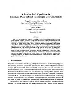
We used well known Internet topologies to verify the suitability of the algorithms, and randomly generated topologies to verify the computational scalability of the algorithms. The known Internet topologies include NSFNET (14 nodes and 21 edges) [4], ARPANET (20 nodes and 32 edges) [1], and Italian National Network (33 nodes and 67 edges) [1]. As in [3], [7], [13], [14], [28], the edge weights were uniformly generated in a range (we used the range [1, 10]). From our analysis, one should expect our algorithms to perform similarly on various edge weights. For each topology, we used the same (s, t) pair for all algorithms. For a fair comparison with the limited granularity heuristic, we used 1/ as the parameter n in [28]. For each topology, we tested three different values of W : a small value of W such that DMCP(G, s, t, K, W ) is infeasible; a large value of W such that DMCP(G, s, t, K, W ) is feasible; and a larger value of W such that DMCP(G, s, t, K, W/2) is feasible. We performed the tests with K = 3. For NSFNET, we first set W to 5 (the small value of W ). FPTAS-SMCP, FPTAS-FMCP and K-Approx were all able to find a path whose three path weights are 20, 20, 14, for each of  ∈ {1.0, 0.5, 0.2, 0.1}. However, RANDOM, LGRANU and L-GRANU2 all failed to find any path. Next, we set W = 20. This time, RANDOM was able to find a path with path weights 20, 20, 14. L-GRANU2 was able to find a path with path weights 19, 21, 23 for  = 0.5, 0.2. For  = 0.1, LGRANU2 was able to find a path with path weights 20, 20, 14. However, L-GRANU still failed to find a path. Finally, we set W = 40. This time, all algorithms were able to find a path. Figure 1(a) illustrates the quality of the paths found (with  = 0.5), where the y-axis measures the maximum ratio of the path weight over the path constraint for the path found by the different algorithms. In case no path was found, we treat this ratio as infinity. Figures 1(b) and 1(c) illustrate the results for ARPANET and Italian National Network respectively. We can see that in all cases, FPTAS-SMCP, FPTAS-FMCP and Approx find a good path. Figure 2(a) illustrates the running times (in seconds) of the different algorithms, as well as their dependency on the value of W , using the case of  = 0.5 for Italian National Network. As expected, K-Approx and RANDOM are always the fastest. Also, we observe that both FPTAS-SMCP and FPTAS-

FMCP are much faster than L-GRANU and L-GRANU2. As expected, the running time of FPTAS-SMCP is independent of W , while the running time of FPTAS-FMCP is either slightly larger than that of FPTAS-SMCP (when W is small), or very small (when W is large). We also observe that the running times of L-GRANU and L-GRANU2 may increase with W slightly, but not significantly. This is due to the fact that more edge relaxations may be performed by LGRANU and L-GRANU2 for larger values of W . Figure 2(b) illustrates the running times (in seconds) of our two FPTASs as functions of , using the case of W = 5, 35 for Italian National Network. As expected, the running times increase with 1 . Again, we note that the running time of FPTAS-SMCP is independent of W , while the running time of FPTAS-FMCP is either slightly larger than that of FPTASSMCP (for small W ) or very small (for large W ). To study the scalability of our FPTASs with the network size, we also tested FPTAS-SMCP and FPTAS-FMCP on large network topologies generated by BRITE, a well known Internet topology generator [2]. The values of W were chosen similarly as in the case of well known topologies. We report results with  = 0.5 for all topology sizes for illustration. BRITE provides several well-known models (including the Waxman model [24]) for generating reasonable network topologies. We adopted the Waxman model (with default parameters provided by BRITE) to generate random networks. We used five different numbers of nodes: 80, 100, 120, 140, 160. Correspondingly, BRITE generated five network topologies with the following sizes: (1) 80 nodes with 314 edges, (2) 100 nodes with 390 edges, (3) 120 nodes with 474 edges, (4) 140 nodes with 560 edges, (5) 160 nodes with 634 edges. For each topology, we ran 10 test cases. For each test case, we randomly generated a source-destination node pair (s, t) and used this pair for all tested algorithms. For this node pair, we used a small value of W and a large value of W to test the algorithms (note that these values of W may change when the node pair changes). The running times of our algorithms are shown in Figure 2(c), where the running time shown for each algorithm is the average over 10 cases, where the largest standard deviation is 1.29. We observe that the running times of all algorithms (expect

GUOLIANG XUE ET AL.: FINDING A PATH SUBJECT TO MANY ADDITIVE QOS CONSTRAINTS

80 SMCP W=5 SMCP W=35 FMCP W=5 FMCP W=35

5

70

2.5 2 1.5

4

3

2

1

5

W

35

70

(a) Running time vs W Fig. 2.

50 40 30 20

1

0.5 0

SMCP(small W) SMCP(large W) FMCP(small W) FMCP(large W)

60 Running Time (sec)

Running Time (sec)

3

6

SMCP FMCP K−Approx Random L−GRANU L−GRANU2

Running Time (sec)

4 3.5

9

0

10

0.1

0.2

0.5

ε

(b) Running time vs 

1

0 80

100

120

140

160

n (c) Running time vs n

Running time vs various factors.

that of FPTAS-FMCP with large W ) increase with the increase of the network size. For the random networks generated, m is approximately 4n. Since we used K = 3 and  = 0.5, the running times of both FPTAS-SMCP and FPTASn 2 ) ) = O(n3 ) for the cases tested. FMCP should be O(m( 0.5 For small values of W , FPTAS-FMCP may have to solve 2UB c = 6 in instances of RMCP with τ set to 7H (note that b LB· blog2 (n−1)c this case) for H = 1, 2, 4, . . . , 2 , n − 1. Note that for the same setting, FPTAS-SMCP only needed to solve one instance of RMCP with τ set to 7(n − 1). Since the running time of PseudoRMCP is proportional to τ K−1 , we can use 1 + [1 + 14 + ( 14 )2 + ...] = 37 as an estimate of the maximum of the ratio of the running time of FPTAS-FMCP over the running time of FPTAS-SMCP. Figure 2(c) conforms to this analysis. In terms of running time, most heuristic algorithms are fast, but do not guarantee quality of solutions. There could be situations where they will produce solutions that deviate from the optimal solutions to a considerable extent. So, RANDOM is quite fast since it requires K +1 shortest path computations. K-Approx is the fastest since it requires only one shortest path computation. We note that K-Approx produces solutions better than or as good as the solutions produced by RANDOM whenever the latter is successful. FPTASs take more time as the value of  chosen becomes smaller. In other words, the more accuracy required for the solution, the more is the time taken. This is not surprising since FPTASs provide guarantees on the accuracy of the solutions produced. This guarantee requirement is the reason for large running times taken by the FPTASs. K-Approx is a constant factor approximation algorithm with the constant equal to the number of edge weights. However, simulation results in comparison with those of our FPTASs which guarantee accuracy of the solutions (specified arbitrarily by the value of ), provide evidence that K-Approx performs quite well in practice. VII. C ONCLUSIONS In this paper, we have studied the MCP problem with K additive QoS constraints, where K ≥ 2 is a fixed constant. We presented a novel O(Km + n log n) time K-approximation algorithm which uses a single auxiliary edge weight to compute a shortest path. Because of this property, the algorithm is

easily implementable in a hop-by-hop environment. We also presented two FPTASs for two slightly different versions of the problem whose time complexities, when reduced to the case of K = 2, compare favorably with existing algorithms. To implement the FPTASs proposed in this paper in the current networking environment, some careful modifications will be necessary. The routing tables will have to store the next hop addresses for every source destination pair for a few discrete values of . These values of  may be used to determine the traffic classes in the network. It may be noted that the results presented in this paper, although derived under the model of an undirected graph, are equally valid for the case of directed graphs. ACKNOWLEDGMENT The authors wish to thank the associate editor and the anonymous reviewers whose valuable comments on earlier versions of this paper helped to improve the quality of the paper significantly. R EFERENCES [1] R. Andersen, F. Chung, A. Sen and G. Xue; On disjoint path pairs with wavelength continuity constraint in WDM networks; IEEE Infocom’04, pp. 524–535. [2] BRITE; http://www.cs.bu.edu/brite/. [3] S. Chen and K. Nahrstedt; On finding multi-constrained paths; IEEE ICC’1998; pp. 874–879. [4] X. Chu and B. Li, Dynamic routing and wavelength assignment in the presence of wavelength conversion for all-optical networks; IEEE/ACM Trans.on Networking,Vol.13(2005),pp.704-715. [5] T.H. Cormen, C.E. Leiserson, R.L. Rivest and C. Stein; Introduction to Algorithms; second edition; McGraw Hill, 2001. [6] F. Ergun, R. Sinha and L. Zhang; An improved FPTAS for restricted shortest path; Information Processing Letters; Vol. 83(2002), pp. 287– 291. [7] A. Goel, K.G. Ramakrishnan, D. Kataria and D. Logothetis; Efficient computation of delay-sensitive routes from one source to all destinations; IEEE Infocom’2001; pp. 854–858. [8] R. Guerin and A. Orda; QoS routing in networks with inaccurate information: theory and algorithms; IEEE/ACM Transactions on Networking; Vol. 7(1999), pp. 350–364. [9] R. Hassin; Approximation schemes for the restricted shortest path problem; Mathematics of Operations Research; vol. 17(1992), pp. 36– 42. [10] C. Huitema, Routing in the Internet, 2nd ed., Prentice Hall PTR, 2000. [11] O.H. Ibarra and C.E. Kim; Fast approximation algorithms for the knapsack and sum of subset problems; Journal of the ACM; Vol. 22(1975), pp. 463–468.

GUOLIANG XUE ET AL.: FINDING A PATH SUBJECT TO MANY ADDITIVE QOS CONSTRAINTS

[12] J.M. Jaffe; Algorithms for finding paths with multiple constraints; Networks; Vol. 14(1984), pp. 95–116. [13] A. Juttner, B. Szviatovszki, I. Mecs and Z. Rajko; Lagrange relaxation based method for the QoS routing problem; IEEE Infocom’2001, pp. 859–868. [14] T. Korkmaz and M. Krunz; Mult-constrained optimal path selection; IEEE Infocom’2001; pp. 834–843. [15] D.H. Lorenz and D. Raz; A simple efficient approximation scheme for the restricted shortest path problem; Operations Research Letters; Vol. 28(2001), pp. 213–219. [16] Q. Ma and P. Steenkiste; Quality-of-service routing for traffic with performance guarantees; IWQoS’97, May 1997. [17] M.A. Marsan, G. Corazza, M. Listanti and A. Roveri (eds); Quality of service in multiservice IP networks; Lecture Notes in Computer Science, Vol. 2601, 2003. [18] A. Orda; Routing with end-to-end QoS guarantees in broadband networks; IEEE/ACM Transactions on Networking; Vol. 7(1999), pp. 365– 374. [19] A. Orda and A. Sprintson; Precomputation schemes for QoS routing; IEEE/ACM Transactions on Networking; Vol. 11(2003), pp. 578–591. [20] A. Orda and A. Sprintson; Efficient algorithms for computing disjoint QoS paths; IEEE Infocom’2004; pp. 727–738. [21] S. Sahni; General techniques for combinatorial approximation; Operations Research, Vol. 25(1977), pp. 920–936. [22] Z. Wang and J. Crowcroft; Quality-of-service routing for supporting multimedia applications; IEEE Journal on Selected Areas in Communications; Vol. 14(1996), pp. 1228–1234. [23] A. Warburton; Approximation of Pareto optima in multiple-objective, shortest path problem; Operations Research; Vol. 35(1987), pp. 70–79. [24] B.M. Waxman; Routing of multipoint connections; IEEE Journal on Selected Areas in Communications; Vol. 6(1988), pp. 1617-1622. [25] G. Xue; Primal-dual algorithms for computing weight-constrained shortest paths and weight-constrained minimum spanning trees; IEEE IPCCC’2000; pp. 271–277. [26] G. Xue; Minimum cost QoS multicast and unicast routing in communication networks; IEEE Transactions on Communications; Vol. 51(2003), pp. 817–824. [27] G. Xue, A. Sen and R. Banka; Routing with many additive QoS constraints; ICC’2003: IEEE International Conference on Communications; pp. 223–227. [28] X. Yuan; Heuristic algorithms for multiconstrained quality-of-service routing; IEEE/ACM Transactions on Networking; Vol. 10(2002), pp. 244–256.

10

Guoliang (Larry) Xue (SM’99/ACM’93) received the BS degree (1981) in mathematics and the MS degree (1984) in operations research from Qufu Teachers University, Qufu, China, and the PhD degree (1991) in computer science from the University of Minnesota, Minneapolis, USA. He is a Full Professor in the Department of Computer Science and Engineering at Arizona State University. He has held previous positions at Qufu Teachers University (Lecturer, 1984-1987), the Army High Performance Computing Research Center (Postdoctoral Research Fellow, 1991-1993), the University of Vermont (Assistant Professor, 19931999; Associate Professor, 1999-2001). His research interests include efficient algorithms for optimization problems in networking, with applications to fault tolerance, robustness, and privacy issues in networks ranging from WDM optical networks to wireless ad hoc and sensor networks. He has published over 130 papers in these areas. His research has been continuously supported by federal agencies including NSF and ARO. He received the Graduate School Doctoral Dissertation Fellowship from the University of Minnesota in 1990, a Third Prize from the Ministry of Education of P.R. China in 1991, an NSF Research Initiation Award in 1994, and an NSF-ITR Award in 2003. He is an Editor of Computer Networks (COMNET), an Editor of IEEE Network, and an Associate Editor of the IEEE Transactions on Circuits and Systems-I: Regular Papers, and the Journal of Global Optimization. He has served on the executive/program committees of many IEEE conferences, including Infocom, Secon, Icc, Globecom and QShine. He served as the General Chair of IEEE International Performance, Computing, and Communications Conference in 2005, and will serve as a TPC co-chair of IEEE Globecom’2006 Symposium on Wireless Ad Hoc and Sensor Networks, as well as a TPC co-chair of IEEE ICC’2007 Symposium on Wireless Ad Hoc and Sensor Networks. He also serves on many NSF grant panels and is a reviewer for NSERC (Canada).

Arunabha (Arun) Sen (M’90) received his bachelors degree in Electronics and Tele-Communication Engineering from Jadavpur University, Kolkata, India and PhD degree in Computer Science from University of South Carolina, Columbia, South Carolina. He is currently an Associate Professor in the department of Computer Science and Engineering at Arizona State University. He also serves as the Associate Chairman of the department responsible for Graduate Programs and Research. His research interest is in the area of resource optimization problems in Wireless and Optical networks. He primarily studies the algorithmic issues related to the problems in these domains and utilize graph theoretic and combinatorial optimization techniques to find solutions. He has published over eighty research papers in peer reviewed journals and conferences on these topics. He has served many IEEE and ACM workshops and conferences either as a Program Committee member or as the Chair of the Program Committee.

Weiyi Zhang (S’02) received the B.E. and M.E. degrees from Southeast University, China, in 1999 and 2002 respectively. Currently he is a Ph.D student in the Department of Computer Science and Engineering at Arizona State University. His research interests include reliable communication in networking, protection and restoration in WDM networks, and QoS provisioning in communication networks.

Jian Tang (S’04) received the B.E. and M.E. degrees from Beijing University of Posts and Telecommunications, China, in 1998 and 2001 respectively. Currently, he is a Ph.D candidate in the Computer Science and Engineering Department of Arizona State University. His research interest is in the area of wireless networking and mobile computing with emphases on routing, scheduling and cross-layer design in wireless networks. He is a student member of IEEE.

GUOLIANG XUE ET AL.: FINDING A PATH SUBJECT TO MANY ADDITIVE QOS CONSTRAINTS

Krishnaiyan Thulasiraman (F’90/ACM’95) received the Bachelor’s degree (1963) and Master’s degree (1965) in electrical engineering from the University of Madras, India, and the Ph.D degree (1968) in electrical engineering from IIT, Madras, India. He holds the Hitachi Chair and is Professor in the School of Computer Science at the University of Oklahoma, Norman, where he has been since 1994. Prior to joining the University of Oklahoma, Thulasiraman was professor (1981-1994) and chair (1993-1994) of the ECE Department in Concordia University, Montreal. He was on the faculty in the EE and CS departments of the IITM during 1965-1981. Dr. Thulasiraman’s research interests have been in graph theory, combinatorial optimization, algorithms and applications in a variety of areas in CS and EE: electrical networks, VLSI physical design, systems level testing, communication protocol testing, parallel/distributed computing, telecommunication network planning, fault tolerance in optical networks, interconnection networks etc. He has published more than 100 papers in archival journals, coauthored with M. N. S. Swamy two text books ”Graphs, Networks, and Algorithms” (1981) and ”Graphs: Theory and Algorithms” (1992), both published by Wiley Inter-Science, and authored two chapters in the Handbook of Circuits and Filters (CRC and IEEE, 1995) and a chapter on ”Graphs and Vector Spaces ” for the handbook of Graph Theory and Applications (CRC Press,2003). Dr. Thulasiraman has received several awards and honors: Endowed Gopalakrishnan Chair Professorship in CS at IIT, Madras (Summer 2005), Elected member of the European Academy of Sciences (2002), IEEE CAS Society Golden Jubilee Medal (1999), Fellow of the IEEE (1990) and Senior Research Fellowship of the Japan Society for Promotion of Science (1988). He has held visiting positions at the Tokyo Institute of Technology, University of Karlsruhe, University of Illinois at Urbana-Champaign and Chuo University, Tokyo. Dr. Thulasiraman has been Vice President (Administration) of the IEEE CAS Society (1998, 1999), Technical Program Chair of ISCAS (1993, 1999), Deputy Editor-in-Chief of the IEEE Transactions on Circuits and Systems I ( 2004-2005), Co-Guest Editor of a special issue on ”Computational Graph Theory: Algorithms and Applications” (IEEE Transactions on CAS , March 1988), , Associate Editor of the IEEE Transactions on CAS (1989-91, 19992001), and Founding Regional Editor of the Journal of Circuits, Systems, and Computers and an editor of the AKCE International Journal of Graphs and Combinatorics. Recently, he founded the Technical Committee on ”Graph theory and Computing” of the IEEE CAS Society.

11