Finding Alternative Expression Quantitative Trait Loci by Exploring ...

JOURNAL OF COMPUTATIONAL BIOLOGY Volume 21, Number 5, 2014 # Mary Ann Liebert, Inc. Pp. 385–393 DOI: 10.1089/cmb.2014.0026

Finding Alternative Expression Quantitative Trait Loci by Exploring Sparse Model Space ZHIYONG WANG,1 JINBO XU,1 and XINGHUA SHI 2

ABSTRACT Sparse modeling, a feature selection method widely used in the machine-learning community, has been recently applied to identify associations in genetic studies including expression quantitative trait locus (eQTL) mapping. These genetic studies usually involve high dimensional data where the number of features is much larger than the number of samples. The high dimensionality of genetic data introduces a problem that there exist multiple solutions for optimizing a sparse model. In such situations, a single optimization result provides only an incomplete view of the data and lacks power to find alternative features associated with the same trait. In this article, we propose a novel method aimed to detecting alternative eQTLs where two genetic variants have alternative relationships regarding their associations with the expression of a particular gene. Our method accomplishes this goal by exploring multiple solutions sampled from the solution space. We proved our method theoretically and demonstrated its usage on simulated data. We then applied our method to a real eQTL data and identified a set of alternative eQTLs with potential biological insights. Additionally, these alternative eQTLs implicate a network view of understanding gene regulation. Key words: expression quantitative trait locus (eQTL) mapping, redundancy, sparse modeling.

1. INTRODUCTION

D

iscovering the relationship between genetic variation and molecular traits, such as gene expression levels, is an essential step for understanding cellular functions at a systems level. Identifying expression quantitative trait loci (eQTLs) through eQTL mapping is one of such endeavors in search of genetic variation that is associated with changes in gene expression levels. An association in eQTL mapping is primarily reflected by a statistical correlation between the genotypes of a genetic variant and the expression levels of the corresponding gene in the samples. These eQTL associations provide a hypothesis that there is some underlying regulatory mechanism for further investigation. (Montgomery et al., 2010; Pickrell et al., 2010; Schlattl et al., 2011; Shabalin, 2012; Stegle et al., 2010; Fusi et al., 2012; Stranger et al., 2007; Stranger et al., 2012). Many methods have been proposed for eQTL mapping, including a recent propagation of machinelearning approaches (Chen et al., 2012; Kim and Xing, 2012; Lee and Xing, 2012; Fusi et al., 2012; Lee et al., 2010; Wang et al., 2011). These methods either separately examine if the correlation of each pair 1

Toyota Technological Institute at Chicago, Chicago, Illinois. Department of Bioinformatics and Genomics, University of North Carolina at Charlotte, Charlotte, North Carolina.

2

385

386

WANG ET AL.

of traits and genetic variants is significant or characterize their associations as parameters in a machinelearning model. Least absolute shrinkage and selection operator (Lasso) (Tibshirani, 1996) methods, as a type of commonly used machine-learning method, add an l1 norm regularization term to the loss function, leading to a sparse model that favors a sparse solution with a small number of nonzero terms. The sparsity of these algorithms is justified with an assumption that there are only a small number of associations between genetic variant and traits, given an overwhelmingly large number of variant and trait pairs for genome-wide eQTL mapping. In a solution of Lasso model fitted on observed data, the parameters represent the effect of each genetic variant on a particular trait, and those nonzero terms correspond to the identified eQTL associations. However, neither the pair-wise correlation method nor the Lasso model captures the relationship among the expression levels of multiple genes. Hence, multitask Lasso models (Chen et al., 2012; Lee and Xing, 2012; Lee et al., 2010) were proposed to impose sparsity over all of the variant and trait pairs to take consideration of related genes. In both Lasso and multitask Lasso models, the weights of genetic variants are computed from an optimization model with its original loss function and l1 norm of the parameters. Solving the optimization problem results in a solution with the sparse property containing only a limited number of nonzero parameters. The sparseness can be controlled by changing the coefficient of the regularization term. These optimization-based methods have the same assumption that the optimization problem has a single global optimal solution. However, the solution from Lasso methods may be inconsistent in either theory (Zou, 2006) or real situation. In eQTL mapping, the data is usually high dimensional, where the number of genetic variants is much larger than the number of samples, and hence there exists multiple solutions with the same optimal value. In such situations, the solutions resulting from different initializations are inconsistent in terms of the nonzero support of the weights. Thus, the result from a single run of these methods is unreliable, although such a simplistic approach has been widely applied in eQTL mapping. The sparse assumption in these models is also problematic in modeling biological data, since biological systems typically contain redundant and backup mechanisms. (Fishman-Lobell et al., 1992; Korn et al., 2007). Nonetheless, biological redundancy is seldom taken into account in eQTL mapping. In this article, we propose a novel method to finding the alternative relationship between genetic variants and traits, which shows the redundancy of two genetic variants to a particular trait. Instead of studying a single optimization result, our method explores the space of the optimization solutions by repeatedly running the Lasso method with random initialization parameters. From this randomly sampled solution set, our method has the capability to extract not only the strength of each pair of genetic variant and trait, but also the relationship of two eQTLs regarding their effects on a given trait. We demonstrate the capability of our method both theoretically by a mathematical proof and practically using simulation data. We further apply our method to a real human eQTL data set and find a set of alternative eQTLs with potential biological insights. The remaining article is organized as follows: We describe our method in Section 2, present the results in Section 3, and conclude the article with discussions in Section 4.

2. METHOD 2.1. Problem definition We denote X as the observed genotypes of the genetic variants, with D columns for D variants and N rows for N samples. We denote Y as the phenotype data, with P columns for P traits and N rows for N samples. For eQTL mapping, Y includes the expression profiles of all the genes in the samples under investigation. The method of sparse modeling is to find the optimal matrix B with D rows and P columns by minimizing the following square loss function plus a regularization term. L(X‚ Y‚ B) = kY - XBk2 + kkBkq

(1)

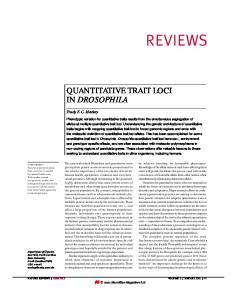
The Lasso method is a special case with q = 1. With l1-norm, a Lasso model favors a sparse result with a small number of nonzero terms (Candes et al., 2008). In practical situations, there are two cases when multiple solutions exist for a Lasso model, as illustrated in Figure 1. As illustrated in Figure 1A, the loss function needs to be symmetric along the line of x = y. In eQTL mapping, the symmetry can be interpreted as two alternative genetic variants with redundant effect on gene expression. Therefore, we utilize this property to find alternative eQTLs, corresponding genes, or even

FINDING ALTERNATIVE EQTLS BY EXPLORING SPARSE MODEL SPACE

387

FIG. 1. Optimal solutions defined by the contour lines of the loss function and the regularization term. The axes of X and Y correspond to two weights of a solution. Dotted and solid ellipses and lines are the contour of the loss function, and gray boxes show the contour of l1 regularization term. (A) A strict convex loss function and l1 regularization term, with optimization error. (B) A nonstrict convex loss function and l1 regularization term.

pathways that perform a backup function for system robustness. In this article, we aim to find such variant pairs that are redundant to each other, by investigating multiple solutions sampled from the solution space.

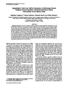
2.2. Our method The existence of multiple optimization solutions in eQTL mapping prevents us from using a single optimized sparse model to explain the importance of features. In order to investigate the model solution space, we therefore propose a sampling method to generate a set of solutions that is expected to be a representative set covering all the multiple solutions. Consequently, we compute the covariance of the solution vectors as an approximation for the alternative relationship between two genetic variants in eQTL mapping. These identified alternative eQTLs represent a redundant relationship regarding their effect on gene expression. Our method shown in Figure 2 can be summarized as follows. First, we search for an optimal l1 regularization coefficient, k, by carrying out a five-fold cross validation. Second, we sample M initialization,

FIG. 2. The flowchart of our method. From a given eQTL data set with genotypes of genetic variants and expression profiles of genes, our method first finds the coefficient of the regularization term, k, by a 5-fold cross validation. Then, our method samples M models through parameter estimation with different initializations. From the M models, our method finally screens for alternative eQTLs. eQTL, expression quantitative trait locus.

388

WANG ET AL.

(M) B0(1) ‚ B(2) 0 ‚ . . . ‚ B0 independently from a uniform distribution. With these initialization values and k, we then run Lasso M times and produce M models: B(1) ‚ B(2) ‚ . . . ‚ B(M) . For each pair of genetic variants, we compute the correlation coefficient of their weights in M solutions. Finally, we extract the pairs whose correlation coefficients are equal to or greater than a cutoff c1 and each of whom has more than c2 nonzero values out of M models. These extracted pairs are considered as alternative eQTLs that influence the expression levels of a particular gene. Our method can be justified in theory by the following claim. Here we describe the claim in a plain way, and the rigorous description and its proof can be found in Supplementary Material (Supplementary Material is available online at www.liebertpub.com/cmb). (2) (M) (2) (M) Claim: Denote b(1) and b(1) as the weights of two features i and j. The i ‚ bi ‚ . . . bi j ‚ bj ‚ . . . bj (1) (2) (M) (1) (2) correlation coefficient of bi ‚ bi ‚ . . . bi and bj ‚ bj ‚ . . . b(M) among all the M sampled models is j negative when the two features have the same effect on the responding variable.

A sketch proof: The claim that two alternative features have the same effect on the responding variable can be viewed the same as the claim that we can exchange the value of the two features, but the responding value is kept the same. From this symmetry, we can derive the conclusion that if b1 ::bi ::bj ::bp is an optimal solution, b1 ::bi ::bj ::bp is also an optimal solution. Therefore, all the solutions of the optimization problem are paired, which implies that the correlation coefficient of bi and bj is negative. We now justify our method by performing an analysis of suboptimal solution. Optimization methods may produce a solution with error caused by either the numerical precision or the convergence tolerance. We denote B* as the optimal solution, and Be as the solution with some small error e, such that jL(X‚ Y‚ B ) - L(X‚ Y‚ Be )j < e. We assume that the loss function L(X,Y,B) has a lower bounded Lipschitz on the difference between a suboptimal solution and an optimal solution. The lower bound is denoted as u1. jL(X‚ Y‚ B ) - L(X‚ Y‚ Be )j qu1> 0 kB - Be k2 Then we have a bound for Be dependent on the error of loss function. kB - Be k2