Jun 28, 2006 - Various approaches for keyword proximity search have been implemented in .... how to do this reduction so that the optimization problem.
Finding and Approximating Top-k Answers in Keyword Proximity Search∗ [Extended Abstract] Benny Kimelfeld and Yehoshua Sagiv The Selim and Rachel Benin School of Engineering and Computer Science, The Hebrew University Edmond J. Safra Campus, Jerusalem 91904, Israel
{bennyk,sagiv}@cs.huji.ac.il ABSTRACT
1.
Various approaches for keyword proximity search have been implemented in relational databases, XML and the Web. Yet, in all of them, an answer is a Q-fragment, namely, a subtree T of the given data graph G, such that T contains all the keywords of the query Q and has no proper subtree with this property. The rank of an answer is inversely proportional to its weight. Three problems are of interest: finding an optimal (i.e., top-ranked) answer, computing the top-k answers and enumerating all the answers in ranked order. It is shown that, under data complexity, an efficient algorithm for solving the first problem is sufficient for solving the other two problems with polynomial delay. Similarly, an efficient algorithm for finding a θ-approximation of the optimal answer suffices for carrying out the following two tasks with polynomial delay, under query-and-data complexity. First, enumerating in a (θ + 1)-approximate order. Second, computing a (θ + 1)-approximation of the top-k answers. As a corollary, this paper gives the first efficient algorithms, under data complexity, for enumerating all the answers in ranked order and for computing the top-k answers. It also gives the first efficient algorithms, under query-and-data complexity, for enumerating in a provably approximate order and for computing an approximation of the top-k answers.
Typically, the aim of keyword search is to find chucks of text that are relevant to the keywords. Sometimes, there is also an underlying structure that can be taken into account when ranking answers, e.g., PageRank [3]. In keyword proximity search, however, not only does the structure influence the ranking process—it is also part of the answer. As an example, when searching for the keywords “Vardi” and “Databases” in DBLP, one answer might be a paper on databases written by Vardi while another could be a journal on databases that includes a paper with Vardi as an author. Only the structure, as opposed to just the occurrences of the keywords and the surrounding text, can indicate the full meaning of the answer. Typically, the structure can be represented as a graph, where keywords constitute some of the nodes, while other nodes as well as the edges indicate the structure. An answer is a subtree that includes the keywords of the query. By assigning weights to edges and possibly to nodes, answers that represent different types of associations between the keywords can be ranked apart. Several systems for keyword proximity search have been implemented in recent years. DBXplorer [1], BANKS [2, 14] and DISCOVER [11] support keyword search in relational databases. These systems represent data as a graph, where nodes correspond to tuples and keywords. Edges connect tuples to each other, according to foreign keys, and also connect tuples with the keywords appearing in those tuples. XKeyword [12] implements a similar approach for XML. In the “information unit” approach of [20] for searching the Web, the aim is somewhat different—representing an answer as a collection of pages that include the given keywords, rather than just a single page. Although these systems use different techniques, it was shown in [16] that they actually solve variants of the same graph problem. The above systems implement algorithms that are based on heuristics, in an attempt to reduce the search space. In some of these systems, the efficiency is further enhanced at the cost of generating the answers in an “almost,” rather than the exact, ranked order. In the worst case, however, the runtime is exponential, even if the size of the query is bounded and there are only a few answers.1 The rationale for using a heuristic approach is the intractability of finding the top-ranked answer (because the Steiner-tree problem is NP-hard). However, two questions naturally arise. First, if
Categories and Subject Descriptors: F.2.2 [Nonnumerical Algorithms and Problems]: Computations on discrete structures; H.3.3 [Information Search and Retrieval]: Search process; H.2.4 [Systems]: Query processing General Terms: Algorithms Keywords: Keyword proximity search, top-k answers, approximations of top-k answers ∗This research was supported by The Israel Science Foundation (Grants 96/01 and 893/05).
Permission to make digital or hard copies of all or part of this work for personal or classroom use is granted without fee provided that copies are not made or distributed for profit or commercial advantage and that copies bear this notice and the full citation on the first page. To copy otherwise, to republish, to post on servers or to redistribute to lists, requires prior specific permission and/or a fee. PODS’06, June 26–28, 2006, Chicago, Illinois, USA. Copyright 2006 ACM 1-59593-318-2/06/0003 ...$5.00.
1
INTRODUCTION
The algorithm used in BANKS is an exception, since it has a polynomial delay, under data complexity, but it neither finds all the answers nor guarantees an approximate order.
the size of the query is bounded, the Steiner-tree problem is tractable [8, 5]. So, can the top-k answers be computed efficiently under data complexity? Second, can the vast amount of approximation algorithms for Steiner-trees (e.g., [4, 10, 9, 18, 25, 21]) be used in order to find an approximation (as defined in [7]) of the top-k answers? In this paper, we show that the answer to both questions is positive. We measure the runtime of an enumeration algorithm in terms of the delay, that is, the length of time between generating two successive answers. An algorithm is efficient if it enumerates answers with polynomial delay (i.e. polynomial in the size of the input). Our results hold within the formal framework defined in Section 2 and are divided into two cases: exact answers and approximations; in the first case, the query is assumed to be of a fixed size. For both cases, we show that an efficient algorithm A for finding just one answer is sufficient for enumerating all the answers with polynomial delay. The enumeration is either in ranked order or in an approximate order, depending on whether A computes the top-ranked answer or only an approximation thereof. It follows that either the top-k answers or their approximations can be computed in time that is linear in k and polynomial in the size of the input. Our first result (i.e., enumerating in ranked order) is based on three reductions. We start by adapting the general procedure of Lawler [19] to our case, thereby reducing the problem of enumerating in ranked order to the problem of finding an optimal answer under constraints. In Section 4, we show how to do this reduction so that the optimization problem is a tractable one. In Section 5, we describe algorithms for computing a supertree that includes some node-disjoint subtrees; these algorithms use a reduction to finding Steiner trees. In Section 6, we reduce the optimization problem of Section 4 to the problem of finding a minimal supertree. For our second result, we show that Lawler’s procedure can be used for enumerating in an approximate order. It is also necessary, however, to modify the sequence of reductions, as described in Section 7. There are actually three variants of each of our two results. The formal framework (Section 2) and the exposition of the results (Section 3) are described for all three variants, but the algorithms themselves are given only for the directed case (i.e., answers are directed subtrees).
2. THE FORMAL SETTING 2.1 Enumerations and Top-k Answers An instance of an enumeration problem consists of an input x and a finite set A(x) of answers. An enumeration algorithm E prints all the answers of A(x) without repetitions. We assume that there is an underlying ranking function that maps answers to positive real numbers. The rank of an answer a is denoted by rank (a). Suppose that the algorithm E enumerates the sequence a1 , . . . , an . If rank (ai ) ≥ rank (aj ) holds for all 1 ≤ i ≤ j ≤ n, then the enumeration is in ranked order. The delay of E is the length of time (i.e., execution cost) between printing two successive answers. There is also a delay at the beginning, i.e., until the first answer is printed, and at the end, i.e., until the algorithm terminates after printing the last answer. Formally, the ith delay (1 ≤ i ≤ n) starts immediately after printing the (i − 1)st answer (or at the beginning of the execution if i = 1) and ends when the ith answer is printed; the (n + 1)st delay is
ESA Oslo
t8
t10
t7 Norway
t4 t2
t3
t9
EU
t1
t5
t6
Antwerp
Monarchy Brussels
Belgium
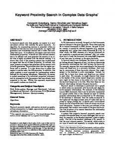
Figure 1: Data graph G1 the delay at the end. We say that E enumerates with polynomial delay [13] if there is a polynomial in the size of the input that bounds the ith delay for all i. There are two related problems. First, finding an optimal (i.e., top-ranked ) answer, that is, printing an answer that has the highest rank (or ⊥ if there is no answer at all). Second, finding the top-k answers (or all the answers if they are fewer than k). An optimal answer is found efficiently if the runtime is polynomial in the size of the input x. Typically, an algorithm for finding the top-k answers is considered efficient if the runtime is polynomial in the size of the input x and the value of k (rather than the size of its binary representation). Note that the runtime is at least linear in k and, in principle, k may be larger than the size of x. Given an algorithm E that enumerates in ranked order with polynomial delay, we can obtain an efficient algorithm for finding the top-k answers by stopping the execution after generating k answers. In particular, we can use E for finding efficiently an optimal answer. There are two important advantages to such an approach. First, the running time is always linear in k (and polynomial in x). Second, k need not be known in advance (hence, the user can decide whether more answers are required, based on the first ones).
2.2
Approximations
Sometimes, for the sake of efficiency, we are interested in approximations. The quality of an approximation is determined by an approximation ratio θ > 1 (θ may be a function of the input x). Given an input x, a θ-approximation of an optimal answer is any answer app ∈ A(x), such that θ·rank (app) ≥ rank (a) for all answers a ∈ A(x); if A(x) = ∅, then ⊥ is a θ-approximation. Following Fagin et al. [7], a θapproximation of the top-k answers is any set AppTop consisting of min(k, |A(x)|) answers, such that θ · rank (a) ≥ rank (a′ ) holds for all a ∈ AppTop and a′ ∈ A(x) \ AppTop. Enumerating all the answers in a θ-approximate order means that if one answer precedes another, then the first one is at most θ times worse than the other one. More formally, the sequence of all answers a1 , . . . , an is in a θ-approximate order if θ · rank (ai ) ≥ rank (aj ) for all 1 ≤ i ≤ j ≤ n. An algorithm that enumerates in a θ-approximate order with polynomial delay can also find efficiently a θ-approximation of the top-k answers, by stopping the execution after printing k answers. In particular, it can find efficiently a θapproximation of an optimal answer.
2.3
The Data Model
A data graph G consists of a set V(G) of nodes and a set E(G) of edges. Nodes are divided into two types: S(G) is the set of structural nodes and K(G) is the set of keyword nodes (or keywords for short). Unless explicitly stated otherwise,
F1 t6
t3
F2 t9
EU
t1
Brussels t1
t3
t6
Belgium
EU Belgium
Brussels
F4 Monarchy
F3 t4 t8
t10
t1
t2
t1
In particular, a top-ranked Q-fragment has the minimum weight. Since we always assume that queries have at least two keywords, the weight of a Q-fragment is not zero.
t2
Norway Belgium
Norway Belgium
Figure 2: Four fragments of G1
edges are directed, i.e., an edge is a pair (n1 , n2 ) of nodes. Keywords have only incoming edges, while structural nodes may have both incoming and outgoing edges. Hence, no edge can connect two keywords. These restrictions imply that E(G) ⊆ S(G) × V(G). For example, consider the data graph G1 depicted in Figure 1. Filled circles represent structural nodes and keywords are written in typewriter font. The weight function wG assigns a positive weight wG (e) to every edge e ∈ E(G). The weight of the data graph G, denoted by w(G), is the sum of the weights of all its edges, P i.e., w(G) = e∈E(G) wG (e). In the examples of this paper, we assume that all edges have an equal weight and, hence, that weight is not shown explicitly. An undirected subtree of a data graph G is a connected subgraph without cycles, assuming that edges are undirected. A directed subtree T of G has a node r, called the root, such that every other node of T is reachable from r through a unique directed path. We use root(T ) to denote the root of T and leaves(T ) to denote the set of all the leaves of T , i.e., the set of all nodes that have no outgoing edges. Consider a subset U of the nodes of a data graph G, where |U | > 1. A directed (respectively, undirected) subtree T of G is reduced w.r.t. U if T contains U , but no proper directed (respectively, undirected) subtree of T also contains U . Note that if U consists of keyword nodes, then a directed subtree T is reduced w.r.t. U if and only if leaves(T ) = U and root(T ) has more than one child. A directed (respectively, undirected) Steiner tree for U is a minimal-weight directed (respectively, undirected) subtree of G that contains U .
3.
A SUMMARY OF THE MAIN RESULTS
Our main results are algorithms for enumerating DQFs, UQFs and SQFs. In this section, we summarize their complexity. First, note that optimal answers correspond to Steiner trees. Specifically, the top-ranked DQF and UQF are directed and undirected Steiner trees, respectively, while the top-ranked SQF corresponds to a group Steiner tree. Finding Steiner trees is intractable under query-and-data complexity, that is, when the size of the query is unbounded. In many cases, however, data complexity [22] is more suitable for measuring the efficiency of algorithms for answering queries. Under this notion, the size of the query Q is assumed to be fixed (note that the number of answers could still be exponential in the size of the data graph). The following theorem shows that, under data complexity, all three types of Q-fragments can be enumerated in ranked order with polynomial delay. The algorithms for DQFs, UQFs and SQFs are reductions to algorithms that solve the corresponding Steiner-tree problems; hence, any algorithm for Steiner trees can be used. In [15], we show how the algorithm of Dreyfus and Wagner [5] for finding undirected Steiner trees can be adapted to the directed and the group variants. Our results for enumerating in ranked order use the running times given in [15]. We assume that the data graph G has n nodes and e edges. The number of keywords in the query Q is denoted by q. We use ni to denote the number of nodes in the ith generated Q-fragment (i.e., the one that is printed at the end of the ith delay). Note that for the last delay (which ends when the algorithm terminates), we assume that ni = 0. Theorem 3.1. Given a data graph G and a query Q, either all DQFs, all UQFs or all SQFs can be enumerated in ranked order with polynomial delay, under data complexity. The ith delay is O (ni (4q n + 3q e log n)). Corollary 3.1. Under data complexity, the top-k answers (DQFs, UQFs or SQFs) can be efficiently computed.
2.4 Fragments A query is simply a set Q of keywords. Given a data graph G, an answer to Q is a Q-fragment, namely, a reduced subtree of G w.r.t. Q. There are three types of Qfragments: directed Q-fragments (DQFs), undirected Qfragments (UQFs) and strong Q-fragments (SQFs). Fragments of the later type (i.e., SQFs) are UQFs that have keywords only in their leaves (in other words, only structural nodes are incident to two or more edges). As an example, consider again the data graph G1 of Figure 1. Figure 2 depicts four subtrees F1 , . . . , F4 of G1 . Let Q1 be the query {Belgium, Brussels, EU} and Q2 be the query {Belgium, Norway}. F1 and F2 are directed Q1 fragments of G1 . The Q2 -fragment F3 is strong but not directed. The Q2 -fragment F4 is undirected but neither directed nor strong. Note that F4 is also an undirected Q3 fragment, where Q3 = {Belgium, Norway, Monarchy}. We take the common approach (e.g., [11, 20, 12, 1]) that the rank of an answer is inversely proportional to its weight. Thus, for a Q-fragment F , we define rank (F ) = w(F )−1 .
The literature has a lot of work on efficient approximation algorithms for the different types of Steiner trees (see [6] for a detailed review). The next theorem shows that these algorithms can be used for enumerating answers (i.e., either DQFs, UQFs or SQFs) in approximately ranked order with polynomial delay, under query-and-data complexity. Specifically, given an approximation algorithm for Steiner trees, f denotes its running time and θ denotes its approximation ratio. We assume that both f and θ are monotonically nondecreasing functions of their arguments; that is, if n1 ≤ n2 , e1 ≤ e2 and q1 ≤ q2 , then f (n1 , e1 , q1 ) ≤ f (n2 , e2 , q2 ) and θ(n1 , e1 , q1 ) ≤ θ(n2 , e2 , q2 ). Hence, n, e and q can indeed be used as the three arguments of f and θ in the following theorem and corollary. Theorem 3.2. If a θ-approximation of the optimal answer can be found in time f , then all answers can be enumerated in a (θ + 1)-approximate ranked order with polynomial delay. The ith delay is O (ni (f + e log n)).
Corollary 3.2. Under query-and-data complexity, if a θ-approximation of the optimal answer can be found efficiently, then a (θ + 1)-approximation of the top-k answers can be efficiently computed.
Algorithm: Input: Output: 1: 2: 3: 4: 5: 6: 7: 8: 9: 10: 11: 12: 13: 14:
In the remainder of this paper, we describe only the algorithms for enumerating DQFs. Accordingly, in the sequel, “subtrees” are always “directed subtrees.” The conclusion discusses briefly the algorithms for UQFs and SQFs.
4. THE BASIC ALGORITHM Lawler [19] generalized an algorithm of Yen [23, 24] to a procedure for computing the top-k solutions of discrete optimization problems. The algorithm DQFSearch of Figure 3 is an adaptation of Lawler’s procedure to enumerating all DQFs, given a query Q and a data graph G. In this algorithm, a constraint is an edge. A DQF F satisfies a set I of inclusion constraints and a set E of exclusion constraints if it has all the edges of I and none of the edges of E. The algorithm employs a subroutine Fragment(G, Q, I, E) that returns a DQF of G that satisfies both I and E. If no such DQF exists, then ⊥ is returned. The following sections describe two options for implementing this subroutine. One returns a minimal (i.e., optimal) DQF satisfying I and E and the other returns an approximation of such a DQF. We now describe how DQFSearch works, assuming that Fragment returns a minimal DQF. The algorithm DQFSearch uses a priority queue Queue. An element in Queue is a triplet hI, E, F i, where I and E are sets of inclusion and exclusion constraints, respectively, and F is the top-ranked DQF that satisfies both I and E. Priority of hI, E, F i in Queue is based on the rank of the DQF F ; that is, the top element of Queue is a triple hI, E, F i, such that rank (F ) is maximal. The operation Queue.removeTop() removes the top element and returns it to the caller. We assume that operations on the priority queue take logarithmic time in the size of Queue, i.e., polynomial time in the size of the input. The algorithm DQFSearch(G, Q) starts by finding, in Line 2, a DQF F that satisfies the empty sets of inclusion and exclusion constraints. Thus, F is the top-ranked DQF. In Line 4, the triplet h∅, ∅, F i is inserted into Queue. In the main loop of Line 5, the top triplet hI, E, F i is removed from Queue in Line 6. In principle, the algorithm should add to Queue the second DQF, in ranked order, among all those satisfying both I and E. But instead of doing that, the algorithm partitions the set comprising all the DQFs satisfying I and E, except for the top-ranked DQF F , and adds the top-ranked DQF of each partition to Queue. The partitioning is done as follows. Let e1 , . . . , ek be the edges of F that are not in I. The ith partition (1 ≤ i ≤ k) is obtained by adding the first i − 1 edges e1 , . . . , ei−1 to I and adding the ith edge ei to E, thereby creating the new sets of constraints Ii and Ei , respectively. In Line 11, these sets are given as arguments to Fragment and the top-ranked DQF Fi that satisfies Ii and Ei is returned. In Line 13, hIi , Ei , Fi i is added to Queue, provided that Fi 6= ⊥. Note that F1 , . . . , Fk are all different from F , since they satisfy constraints that F itself does not satisfy. The DQF F is printed at the end of the iteration, in Line 14. DQFSearch(G, Q) enumerates all DQFs of G. The delay and the order of the enumeration are determined by the implementation of Fragment. Lawler’s procedure [19] was
DQFSearch A data graph G, a query Q All DQFs
Queue ← an empty priority queue F ← Fragment(G, Q, ∅, ∅) if F 6=⊥ then Queue.insert(h∅, ∅, F i) while Queue 6= ∅ do hI, E, F i ← Queue.removeTop() let {e1 , . . . , ek } = E(F ) \ I for i = 1 to k do Ii ← I ∪ {e1 , . . . , ei−1 } Ei ← E ∪ {ei } Fi ← Fragment(G, Q, Ii , Ei ) if Fi 6=⊥ then Queue.insert(hIi , Ei , Fi i) print(F )
Figure 3: Basic algorithm for enumerating DQFs devised for the purpose of finding the top-k answers. The following theorem shows that our adaptation of that procedure indeed enumerates in ranked order provided that Fragment returns optimal answers. Interestingly, DQFSearch(G, Q) can also enumerate in a θ-approximate order if Fragment returns θ-approximations. The theorem also specifies the delay in terms of the running time of Fragment. Recall that n and e are the number of nodes and edges of G, respectively, q is the number of keywords in Q and ni is the number of nodes in the ith generated DQF. Note that there are at most 2e DQFs, i.e., i ≤ 2e . Theorem 4.1. Consider a data graph G and a query Q. • The algorithm DQFSearch(G, Q) enumerates all the DQFs of G in ranked order if Fragment(G, Q, I, E) returns a minimal DQF that satisfies I and E. • If the subroutine Fragment(G, Q, I, E) returns a θapproximation of the minimal DQF that satisfies I and E, then the algorithm DQFSearch(G, Q) enumerates in a θ-approximate ranked order. • If the subroutine Fragment(G, Q, I, E) terminates in T (n, e, q) time, then DQFSearch(G, Q) enumerates with O (ni (T (n, e, q) + log(n · i) + ni )) delay.
4.1
Partial Fragments
The task at hand is to efficiently implement Fragment. Handling exclusion constraints is easy and can be done by deleting the edges of E from the data graph G; hence, we ignore these constraints in the rest of the paper. But handling inclusion constraints is generally intractable. It can be shown that it is NP-complete to decide whether there is any DQF (regardless of its rank) that satisfies a single inclusion constraint, even if the query Q has only two keywords. We circumvent this difficulty by modifying the algorithm DQFSearch so that it only generates inclusion constraints of a special form that is defined as follows. Consider a data graph G and a query Q. A partial fragment (PF) is any directed subtree of G. A set of PFs P is called a set of PF constraints if the PFs in P are pairwise node disjoint. If a subtree T of G includes all the PFs of P, then T is actually
v9 v10 T1 v2
u3
v3
u2
v1
v5 r
B
v6
v7 C
A
B
v8
v7
v8 D
v7 2.ReducedSubtree()
v1
Tˆ v5 T2 3.restore()
Figure 4: Data graph G2
v3
v4
A
a G-supertree of P and we also say that T satisfies P. We use leaves(P) to denote the set of leaves in the PFs of P.
There are two types of PFs. A reduced PF (RPF) has a root with at least two children whereas a nonreduced PF (NPF) has a root with only one child. We emphasize that, as a special case, a single node is considered an RPF. Note that an RPF, but not an NPF, is reduced w.r.t. the set of its leaves. We use P|RPF and P|NPF to denote the set of all the RPFs of P and the set of all the NPFs of P, respectively. By Proposition 4.1, the subroutine Fragment should find a DQF that satisfies a given set P of PF constraints, where leaves(P) is a subset of Q. Without loss of generality, we can add to P every keyword in Q \ leaves(P) as a singlenode RPF. Thus, from now on, when looking for a DQF that satisfies a set P of PF constraints, we assume that leaves(P) = Q, where Q is the given query. Note that by Proposition 4.1, P has at most two NPFs. Suppose that T is a G-supertree of P. Note that T is not necessarily a DQF, even if leaves(T ) = leaves(P) = Q, since the root of T may have a single child. Furthermore, if the root belongs to some NPF of P, then it cannot be deleted in order to obtain a DQF. As an example, Figure 4 shows the data graph G2 and two PFs, T1 and T2 , that are surrounded by dotted polygons. Let Q be the query {A, B, C, D} and P be the set of PF constraints {T1 , T2 }. The minimal G2 -supertree of P comprises the nodes and edges of T1 and T2 as well as the edge (v4 , v5 ). Note, however, that this supertree is not a DQF, since its root v1 has only one child. It can be shown that the only DQF that satisfies P is obtained by choosing r to be the root, connecting r to T1 using the path u1 → · · · → u6 → v1 and connecting r to T2 with the edge (r, v5 ). As another example, suppose that T3 is the subtree of G2 that is obtained by adding the edge (v0 , v1 ) to T1 and let P ′ = {T2 , T3 }. Although there is a G2 -supertree of P ′ , no DQF of G satisfies P ′ . Nevertheless, our algorithms for finding DQFs under PF constraints require finding minimal supertrees and approximations thereof. In the next section, we show how it is done.
C
v2
u1
Proposition 4.1. The algorithm DQFSearch can be executed so that for every generated set of inclusion constraints I, the subgraph of G induced by the edges of I forms a set of PF constraints P, such that leaves(P) ⊆ Q and P has at most two PFs.
v6
v5
Output
T1 D
v1
v5 T2 v4
v3
T2 v4
A
1.collapse()
v2
v1
u5 u4
T1
v11
v0 v9
v9
v0
u6
ˆ G
v0
G
B
v6 C
v8
v1
D
v5
Figure 5: Execution example of Supertree
5.
COMPUTING SUPERTREES
In this section, we consider a graph G and a set T of PF constraints. Recall that T consists of subtrees of G that are pairwise node disjoint. We give algorithms for finding a minimal G-supertree of T and an approximation thereof. Both algorithms are based on an algorithm for finding a reduced G-supertree T of T , namely, T is a subtree of G that includes all the PFs of T and has no proper subtree that also includes these PFs. It should be emphasized that the algorithms of this section are applied even when the set T of PF constraints does not necessarily correspond to a query, that is, the leaves of T need not be keywords. Finding a reduced G-supertree of T is a three-step process. ˆ by collapsing First, G is transformed into a new graph G ˆ each PF of T into a single node. Second, in the new graph G, we find a reduced subtree Tˆ w.r.t. the nodes that correspond to the PFs of T . Third, the PFs of T are restored in Tˆ. We start by describing the operations collapse and restore.
5.1
Collapsing and Restoring Subtrees
Consider a data graph G and a set T of PF constraints. We delete from G all edges e, such that e enters a nonroot node of some PF T ∈ T and e is not an edge of T . The reason for deleting these edges is that they cannot be included in any G-supertree of T . Thus, from now on we assume that if an edge of G enters a non-root node of some T ∈ T , then that edge belongs to T . The graph collapse(G, T ) is the result of collapsing all the subtrees of T in G and it is obtained as follows. • Delete2 from G all the non-root nodes of PFs of T . (The roots of all the PFs of T remain in the collapsed graph, because these PFs are pairwise node disjoint.) • For all deleted edges (u, v), such that u is a non-root node of a PF T ∈ T but (u, v) is not an edge of T , add the edge (root(T ), v) to collapse(G, T ). The weight of the edge (root(T ), v) is the minimum among the weights of all the edges of G from nodes of T to v. In particular, if (root(T ), v) is already an edge of G, then 2
When deleting a node, its incident edges are also removed.
Algorithm: Supertree Input: A data graph G, a set of PF constraints T Output: A reduced G-supertree of T 1: 2: 3: 4: 5: 6: 7:
ˆ ← collapse(G, T ) G R ← {root(T ) | T ∈ T } ˆ s.t. each r ∈ R is reachable from v then if ∃v ∈ V(G) ˆ ˆ R) T ← ReducedSubtree(G, ˆ return restoreG (T , T ) else return ⊥ Figure 6: Finding a reduced G-supertree of T its weight is decreased if there is another edge with a smaller weight from a non-root node of T to v.
As an example, the top part of Figure 5 shows how two nodedisjoint subtrees T1 and T2 are collapsed. These subtrees are surrounded by dotted polygons. In this figure, weights of edges are not specified and we assume that they are equal. (Note that the edges (v3 , B) and (v4 , v6 ) are actually deleted before collapsing T , due to the assumption stated above.) Next, we describe the inverse operation of collapse, namely, ˆ of collapse(G, T ). restoring the subtrees of T in a subgraph H ˆ The data graph restoreG (H, T ) is defined as follows. ˆ • Add all the edges and nodes of T to H. • Consider each PF T of T . For each edge (root(T ), v) ˆ replace this edge with (t, v), where (t, v) has the of H, minimal weight among all edges of G from nodes of T to v. If there are several such nodes t, an arbitrary one is chosen. Note that according to this definition, the edge (root(T ), v) is left unchanged if t = root(T ). As an example, the bottom part of Figure 5 shows how the collapsed subtrees T1 and T2 are restored in Tˆ.
5.2 Approximate and Minimal Supertrees Consider a data graph G and a set T of PF constraints. A reduced G-supertree of T can be obtained as follows. First, collapse all the subtrees of T . Note that only the roots of ˆ Next, find a the PFs of T remain in the resulting graph G. ˆ that is reduced w.r.t. the set R comprising subtree Tˆ of G the roots of the PFs of T . Finally, restore the subtrees of T in Tˆ to obtain a reduced G-supertree of T . The algorithm Supertree of Figure 6 formally describes the above process. Note that in Line 3, a simple test is ˆ has a reduced performed in order to determine whether G ˆ ˆ subtree T w.r.t. R. If the test is positive, T is obtained by ˆ R) in Line 4. executing the procedure ReducedSubtree(G, Figure 5 depicts the graph G and the subtrees T1 and T2 . This figure shows an execution of Supertree for the input ˆ is consisting of G and T = {T1 , T2 }. In the first step, G obtained from G by collapsing the subtrees T1 and T2 . The ˆ that is reduced second step constructs the subtree Tˆ of G w.r.t. the set of roots {v1 , v5 }. Finally, in the third step, T1 and T2 are restored in Tˆ and the result is returned. The proof of correctness of Supertree is omitted, due to a lack of space. Essentially, it is based on the following ˆ w.r.t. R, then observation. If Tˆ is a reduced subtree of G restoring the subtrees of T in Tˆ yields a reduced G-supertree of T . Actually, we can also show the following. If Tˆ is
ˆ a θ-approximation of the directed Steiner tree for R in G, then restoreG (Tˆ, T ) is a θ-approximation of the minimal Gsupertree of T . In particular, if Tˆ is a directed Steiner tree ˆ then restoreG (Tˆ, T ) is a minimal G-supertree of for R in G, T . Thus, we use the algorithm Supertree of Figure 6 as the basis for creating two new algorithms that use existing algorithms from the literature as described below. ˆ R) is an We assume that Approx-DirectedSteiner(G, ˆ existing algorithm that accepts as input a data graph G, ˆ with n ˆ nodes and eˆ edges, and a set R of t nodes of G. It returns a θ(ˆ n, eˆ, t)-approximation of a directed Steiner tree for R in G and its running time is f (ˆ n, eˆ, t).3 As discussed in Section 3, we assume that both θ and f are monotonically non-decreasing functions. The second existing algorithm, ˆ R), returns a directed Steiner tree for DirectedSteiner(G, R in G and its running time is O(3t n ˆ + 2t eˆ log n ˆ ).4 The algorithm Approx-Supertree(G, T ) is obtained by ˆ R), in Line 4 of Figusing Approx-DirectedSteiner(G, ˆ R). The following ure 6, instead of ReducedSubtree(G, theorem shows that Approx-Supertree(G, T ) returns a θ(n, e, t)-approximation of the minimal G-supertree of T . Theorem 5.1. Consider a data graph G and a set T of PF constraints. Suppose that G has n nodes and e edges, and let T have t PFs. Approx-Supertree(G, T ) returns a G-supertree that is reduced w.r.t. T and is a θ(n, e, t)approximation of the minimal G-supertree of T . If no Gsupertree of T exists, then ⊥ is returned. The running time is O(te + f (n, e, t)). The algorithm Min-Supertree(G, T ) is obtained by usˆ R), in Line 4 of Figure 6, instead ing DirectedSteiner(G, ˆ of ReducedSubtree(G, R). The following is a corollary of ˆ R) Theorem 5.1, since the algorithm DirectedSteiner(G, returns a 1-approximation. Corollary 5.1. Consider a data graph G and a set T of PF constraints. Let G have n nodes and e edges, and let T have t PFs. Min-Supertree(G, T ) returns a minimal G-supertree of T if one exists, or ⊥ otherwise. The running time is O(3t n + 2t e log n).
6.
MINIMAL CONSTRAINED ANSWERS
In this section, we show how to find efficiently a minimal DQF that satisfies a set of PF constraints, assuming that the size of the query Q is bounded (otherwise, the problem is intractable). The algorithm Min-Fragment(G, P) of Figure 7 accepts as input a data graph G and a set P of PF constraints, such that leaves(P) = Q. It returns a minimal DQF that satisfies P. If Min-Fragment is used instead of Fragment in Figure 3, then DQFSearch enumerates all the DQFs in ranked order with polynomial delay. (Recall that the arguments of Fragment are converted to those of Min-Fragment as described in Section 4.1.) We use the following notation. For a data graph G and a subset U ⊆ V(G), we denote by G−U the induced subgraph of G that consists of the nodes of V(G) \ U and all the edges 3 We assume that, if necessary, the approximation algorithm is modified so that it returns a reduced subtree w.r.t. R, which can be done in linear time. 4 The specified running time can be obtained by implementing DirectedSteiner as described in [15].
Algorithm: Input: Output: 1: 2: 3: 4: 5: 6: 7: 8: 9: 10: 11: 12: 13: 14:
Min-Fragment A data graph G, a set of PF constraints P, such that leaves(P) = Q A minimal DQF that satisfies P, or ⊥ if none exists
if P consists of a single RPF T then return T if P consists of a single NPF then return ⊥ Fmin ← ⊥ /* — note that the weight of ⊥ is ∞ — */ let T be obtained from P by replacing each N ∈ P|NPF with the PF consisting of root(N ) for all subsets Ttop of T , such that |Ttop | ≥ 2 do /* — Construct the supertree Ttop — */ G1 ← G − ∪N ∈P|NPF (V(N ) \ {root(N )}) − ∪T ∈T \Ttop V(T ) Ttop ← Min-Supertree(G1 , Ttop ) if Ttop 6= ⊥ then /* — Construct the DQF F — */ + let Ttop be the union of Ttop and all N ∈ P|NPF , such that root(N ) ∈ V(Ttop ) + let P ′ be the set of all the PFs of P that are not contained in Ttop + let G2 be obtained from G by removing all the incoming edges of root(Ttop ) + ′ F ← Min-Supertree(G2 , P ∪ {Ttop })
/* — Update Fmin — */ 15: Fmin ← min{Fmin , F } 16: return Fmin Figure 7: Finding a minimal DQF under a set of PF constraints of G between these nodes. If G1 and G2 are subgraphs of G, then G1 ∪ G2 denotes their union, namely, the subgraph G′ that consists of all the nodes and edges that appear in either G1 or G2 ; in other words, G′ satisfies V(G′ ) = V(G1 )∪V(G2 ) and E(G′ ) = E(G1 ) ∪ E(G2 ). Our goal is to find a minimal DQF that satisfies the given set P of PF constraints. Recall that we cannot simply apply the algorithm Min-Supertree of Section 5.2, unless all the PFs of P are actually RPFs. As discussed at the end of Section 4.1, even if we find a minimal G-supertree T of P, a minimal DQF that satisfies P may be very different from T or may not exist at all. Consequently, the algorithm of Figure 7 is more intricate than Min-Supertree. The main idea of the algorithm is to convert P into an + + equivalent set P ′ ∪{Ttop }, such that Ttop is an RPF with the same root as some minimal DQF that satisfies P. We then compute, in Line 14 of Figure 7, a minimal G2 -supertree of + P ′ ∪ {Ttop }, where G2 is obtained from G by deleting the + ) (thereby guaranteeing that edges that enter into root(Ttop + root(Ttop ) is the root of the computed supertree). + In order to understand how we compute Ttop , consider ′ a minimal DQF F that satisfies P. Suppose that for all NPFs N ∈ P, we delete from F ′ all the nodes of N except for root(N ). Next, we delete all the nodes that are not reachable from root(F ′ ). We define the following. ′ • Ttop is the subtree of F ′ that remains after the above deletions. ′+ ′ • Ttop is the subtree of F ′ that is the union of Ttop and ′ all the NPFs N ∈ P, such that root(N ) is in Ttop . ′ • Ttop consists of all PFs T ′ , such that T ′ is either ′+ – an RPF of P that is included in Ttop , or
– root(N ), where N is an NPF of P that is included ′+ in Ttop . • The subgraph G′1 is obtained from G by deleting all nodes n, such that n appears in a PF of P but not in ′ any PF of Ttop . ′+ The following can be shown. First, root(Ttop ) has at least ′ ′ two children. Second, Ttop has at least two PFs. Third, Ttop ′ ′ is a minimal G1 -supertree of Ttop . Fourth, if we replace the ′ ′ subtree Ttop of F ′ with any minimal G′1 -supertree of Ttop , the result remains a minimal DQF that satisfies P. ′ ′ Thus, we can compute Ttop if we know the set Ttop , which is not the case. In the algorithm Min-Fragment of Figure 7, the main loop (Line 7) iterates over all subsets of T ′ that could be the value of Ttop ; in each iteration, the variable Ttop is assigned one possible subset. (The number of these subsets is bounded by a constant assuming that the size of the query is fixed.) Note that T is obtained from P, in Line 6, by replacing each NPF of P with its root. In Line 8, G1 is obtained from G by deleting all the nodes of P that do not appear in Ttop . In Line 9, Min-Supertree finds a minimal G1 -supertree Ttop that satisfies Ttop . It is important to compute the supertree Ttop in the graph G1 , rather than the original graph G, because Ttop cannot use edges and nodes that appear in P but not in Ttop . Note that there could be many minimal G1 -supertrees of Ttop , but Line 9 computes just one such supertree, namely, + Ttop . In Line 11, Ttop is expanded to Ttop by adding the nodes and edges of all NPFs N ∈ P, such that root(N ) is + already in Ttop . Note that Ttop is an RPF. We are now looking for a DQF F that has the same root + + as the RPF Ttop . Note that F must satisfy Ttop as well as all + the PFs of P that are not contained in Ttop . Thus, the set P ′ is constructed in Line 12. To guarantee that F has the same
+ root as Ttop , Line 13 removes from G all the incoming edges of this root and the result is G2 . Line 14 finds a minimal G2 + supertree F that satisfies P ′ ∪ {Ttop }. The algorithm MinFragment returns the minimal F among all those found in the loop of Line 7. The following theorem uses the running time of MinSupertree from Corollary 5.1. Note that Theorem 3.1 follows as a direct corollary, since p ≤ q.
Theorem 6.1. Consider a data graph G with n nodes and e edges. Let Q be a query with q keywords and P be a set of p PF constraints, such that leaves(P) = Q. MinFragment(G, P) returns either a minimal DQF that satisfies P, or ⊥ if there is no such DQF. The running time is O (4p n + 3p e log n). Proof. Suppose that G has a minimal DQF F ′ that satisfies P. We will prove that the algorithm returns a DQF that satisfies P and has a weight that is not larger than that ′ of F ′ . As defined above, F ′ has a subtree Ttop that satis′ fies the PFs of Ttop . Consider the iteration of the loop of ′ Line 7 in which Ttop is assigned the set Ttop . Let Ttop be the minimal G1 -supertree of Ttop that is returned in Line 9 ′ during that iteration. Observe that Ttop and Ttop are not necessarily the same, but the weight of Ttop is not larger ′ than that of Ttop . Since Ttop is a G1 -supertree of Ttop , its root is either a root of some PF of Ttop or a node that does not appear in P. Furthermore, Ttop has none of the edges of the NPFs of P, because G1 has none of these edges. Thus, when Ttop is + expanded to Ttop , the root must have at least two children. It remains to show that Line 14 computes a DQF that satisfies P and has a weight that is not larger than that + by of F ′ . Consider the graph H that is obtained from Ttop ′+ ′ adding all the edges of F that are not in Ttop , i.e., the edges ′+ of the set E(F ′ ) \ E(Ttop ). The graph H has the following properties. First, the weight of H is not larger than that of F ′ . Second, H includes all the PFs of P. Third, the root + of every PF of P is reachable in H from the root of Ttop . Fourth, edges of H that enter non-root nodes of PFs of P must belong to P. Note that these properties continue to hold even if we remove from H all the edges that enter the + root of Ttop (if H indeed has such edges). It thus follows that Line 14 computes a subtree that satisfies all the PFs of P, has a root with at least two children and its weight is not larger than that of F ′ (because H has such a subtree). We have shown that the algorithm returns a minimal DQF that satisfies P if indeed there is such a DQF. The above proof also indicates that if the output is not ⊥, then a DQF that satisfies P is returned. Thus, the algorithm is correct. The running time of Min-Fragment(G, P) is dominated by the two calls to Min-Supertree in Lines 9 and 14. For each subset Ttop ⊆ T of size k, Min-Supertree is called + once with the set Ttop and once with the set P ′ ∪ {Ttop }. + ′ The number of PFs in P ∪ {Ttop } is at most p − k + 1. By Corollary 5.1, an upper bound on the total cost of Lines 9 and 14 is O(g(n, e, p)), where g(n, e, p) = p ` ´` ´ P p k k 3 n + 2 e log n + 3p−k+1 n + 2p−k+1 e log n k
k=2
≤ 4n
p ` ´ P p
k=0
k
3k + 3e log n
p ` ´ P p k 2 = 4n4p + 3e(log n)3p . k
k=0
The specified runtime then follows immediately.
7.
MINIMAL-ANSWER APPROXIMATION
In this section, we show how to find an approximation of a minimal DQF under a set of PF constraints. Note that if, in the algorithm Min-Fragment of Figure 7, we simply replaced Min-Supertree with the algorithm ApproxSupertree of Section 5.2, the running time would still be exponential in the number of PFs of P. Thus, we use the algorithm Approx-Fragment of Figure 8 that accepts as input the data graph G and a set of PF constraints P, such that leaves(P) = Q. This algorithm finds a (θ + 1)approximation of a minimal DQF that satisfies P, given that Approx-DirectedSteiner finds a θ-approximation of a directed Steiner tree. By Proposition 4.1, we can assume that P has at most two NPFs. This fact is important in showing that Approx-Fragment has a polynomial runtime even if the size of the query Q is unbounded. Approx-Fragment starts by checking whether P has no RPFs and, if so, Min-Fragment is applied to the input. Otherwise, a G-supertree Tapp that satisfies P is constructed by the algorithm Approx-Supertree. If Tapp is either a DQF or ⊥, then it is returned by the algorithm. If not, the root of Tapp has only one child (and, hence, root(Tapp ) must also be the root of some NPF of P). We fix this problem by modifying Tapp at the cost of increasing the approximation ratio to θ + 1. This is done as follows. In the loop of Line 7, G′ is obtained from G by deleting all edges e, such that e is not in P and e enters a non-root node of some PF of P (note that the deleted edges cannot be included in any subtree of G that satisfies P). The loop of Line 10 iterates over all RPFs Tr ∈ P and applies MinFragment to G′ and P|NPF ∪ {Tr }. The following can be shown. The minimal subtree Tmin among all those returned by Min-Fragment, during the iterations of the loop, has a root with at least two children and a weight that is not larger than that of the minimal DQF F that satisfies P. Thus, the weight of Tapp ∪ Tmin is at most θ + 1 times the weight of F . Note that Tapp ∪ Tmin is not necessarily a tree (it might even contain directed cycles). However, it can be shown that Tapp ∪ Tmin contains a DQF that satisfies P. The algorithm returns a DQF F that is obtained from Gapp = Tapp ∪ Tmin as follows. Recall that the root of Tapp is reachable from the root of Tmin , since root(Tapp ) is also the root of some NPF of P (or else the algorithm terminates in Line 5). Therefore, root(Tmin ) becomes the root of F unless root(Tmin ) is in some RPF T ∈ P and if so, root(T ) becomes the root of F . Lines 19–22 remove all redundant nodes and edges of Gapp . The loop of Lines 20–21 iterates over all nodes v of Gapp that have more than one incoming edge. Note that such a node v has exactly two incoming edges: one belongs to Tapp and the other is from Tmin . We remove the first and leave the second. Line 22 deletes all structural nodes that have no descendant keywords. Interestingly, the loop of Line 10 can be replaced with a single invocation of Min-Fragment by applying the following transformation to G′ . First, collapse each RPF of P into a single node. Second, add a new keyword v and edges from the collapsed RPFs to v. Min-Fragment is then called with the set P|NPF ∪ {v}. In the next theorem, the runtime analysis assumes that the above optimization is used. As explained in Section 5.2, Approx-Supertree uses Approx-DirectedSteiner and the latter finds a θ-approximation of a directed Steiner tree. The approximation ratio θ and the running time f are mono-
Algorithm: Input: Output:
Approx-Fragment A data graph G, a set of PF constraints P, such that leaves(P) = Q A (θ + 1)-approximation of the minimal DQF that satisfies P, or ⊥ if none exists
1: if P|RPF = ∅ then 2: return Min-Fragment(G, P) /* — Construct Tapp — */ 3: Tapp ← Approx-Supertree(G, P) 4: if Tapp = ⊥ or Tapp is a DQF then 5: return Tapp /* — Construct Tmin — */ 6: G′ ← G 7: for all T ∈ P do 8: remove from G′ all edges (v, u), such that (v, u) ∈ / E(T ) and u ∈ V(T ) \ {root(T )} 9: Tmin ← ⊥ /* — note that the weight of ⊥ is ∞ — */ 10: for all Tr ∈ P|RPF do 11: T ← Min-Fragment(G′ , P|NPF ∪ {Tr }) 12: Tmin ← min{Tmin , T } 13: if Tmin = ⊥ then 14: return ⊥ /* — Remove redundant nodes and edges from Tmin ∪ Tapp — */ 15: r ← root(Tmin ) 16: if r belongs to a subtree T ∈ P|RPF then 17: r ← root(T ) 18: Gapp ← Tmin ∪ Tapp 19: remove from Gapp all incoming edges of r 20: for all nodes v ∈ V(Gapp ) that have two incoming edges e1 ∈ E(Tmin ) and e2 ∈ E(Tapp ) do 21: remove e2 from Gapp 22: delete from Gapp all structural nodes v, such that no keyword is reachable from v 23: return Gapp Figure 8: Finding an approximation of the minimal DQF under a set of PF constraints tonically nondecreasing functions and, hence, n, e and q can be used as their arguments. The constant c denotes the number of NPFs in P; recall that c ≤ 2 whenever ApproxFragment is invoked in Line 11 of DQFSearch (Figure 3). Theorem 7.1. Consider a data graph G with n nodes and e edges. Let Q be a query with q keywords and P be a set of PF constraints, such that leaves(P) = Q and P has at most c NPFs. The algorithm Approx-Fragment(G, P) finds a (θ+1)-approximation of the minimal DQF that satisfies P in O (f + 4c n + 3c e log n) time, where θ and f are the approximation ratio and runtime, respectively, of ApproxDirectedSteiner. Proof. The running time easily follows from that of MinFragment, so we only prove correctness. Suppose that the algorithm is applied to G and P. As discussed above (and using the claim proven below), if the algorithm returns a DQF, then its weight is a (θ + 1)-approximation of a minimal DQF that satisfies P. So, we prove that the algorithm returns a DQF that satisfies P (if one exists) assuming that Line 6 is reached, since the other cases are easy. Consider a minimal DQF F of G that satisfies P. We claim that there is an RPF Tr ∈ P and a subtree T of F , such that T is a reduced supertree of P|NPF ∪ {Tr } and its root has at least two children. Assuming that F exists, this claim implies that Line 15 is reached and the weight of Tmin is not larger than that of F . To prove the claim, consider a minimal subtree T ′ of F that has the same root as F and includes all the NPFs of P. We choose the RPF Tr as follows.
If root(F ) has more than one child in T ′ , then Tr can be any RPF of P. Otherwise, Tr is an RPF that is reachable from root(F ) through an edge that is not in T ′ (note that Tr must exist or else F is not a DQF). Now, we choose T to be the minimal subtree of F that satisfies P|NPF ∪ {Tr }. It remains to show that after executing Line 19–22, Gapp is a DQF that satisfies P. Let G0app be the initial value that is assigned to Gapp in Line 18 and consider the root r that is computed in Lines 15–17. Two properties hold. First, r has two children in G0app , because r is either the root of an RPF (which is included in G0app ) or the root of Tmin (which has two children). Second, all the PFs of P are reachable from r in G0app ; in proof, the root r′ of Tapp is also the root of some NPF of P and, hence, r′ is included in Tmin , which is reachable from r. The first property above clearly continues to hold after deleting (in Line 19) all the incoming edges of r. The same is true for the second property, because of the following case analysis. The root of Tmin is either a node of an RPF R ∈ P, the root of an NPF of P or not in any PF of P. In the first case, r is the root of R, whereas in the other two cases, r is the root of Tmin . Thus, if an edge of P enters r, then r is the root of one PF and also a node of another PF, contradicting the fact that the PFs of P are node disjoint. In Gapp , each non-root node v of a PF T ∈ P has only one incoming edge, namely, the edge of T that enters v. This follows from the facts that Tapp is a subtree that satisfies P and Tmin is a subtree of G′ . Thus, edges of P are not removed in the loop of Line 20. Structural nodes of P are
not deleted in Line 22, because G0app satisfies P, the edges of P are not deleted and all the leaves of P are keywords. If an edge e is removed, then it enters a node n of Tmin but the edge itself does not belong to Tmin .5 Hence, n is still reachable from r after the removal of e. We conclude that the two properties above continue to hold when performing the deletions of edges and nodes in Lines 20–22. At the end of the algorithm, Gapp satisfies the following. First, r is the root of Gapp , because it has no incoming edges and all the nodes of Gapp are reachable from r. Second, each non-root node has just one incoming edge. Third, r has at least two children (because if r is the root of Tmin , then none of the edges of Tmin is removed; and if r is the root an RPF T , then its outgoing edges in T are not deleted). Fourth, the leaves of Gapp are exactly the keywords of Q, since keywords are never deleted from Gapp and, after Line 22, every structural node has a descendant keyword. Fifth, all the PFs of P are included in Gapp . Thus, upon termination, Gapp is a DQF that satisfies P.
8. CONCLUSION The main contribution of this paper is in showing that the answers (i.e., DQFs, UQFs and SQFs) of keyword proximity search can be enumerated in ranked order with polynomial delay, under data complexity. Furthermore, when a faster algorithm is more important than the exact ranked order, it is possible to enumerate in an approximate order with polynomial delay (under query-and-data complexity). It thus follows that the top-k answers as well as approximations thereof (as defined in [7]) can be computed efficiently. In comparison, existing systems [11, 1, 12, 20] use algorithms that have an exponential runtime, in the worst case, even if the size of the query is fixed. Some systems [2, 14, 20] enumerate in an “almost” ranked order, but without proving the existence of any nontrivial approximation ratio (and the delay could still be exponential). It might be argued that our algorithms cannot be effectively implemented in practical systems, because the Steinertree computation must be applied to large graphs. However, our algorithms are efficient reductions in the sense that the Steiner-tree computation dominates the runtime and is applied to graphs that are only slightly different from the original data graph. Any algorithm for enumerating answers, in either the exact or an approximate order, must also solve the corresponding Steiner-tree problem and, so, can be incorporated in our approach. In fact, our reductions show that it is not only necessary but also sufficient to concentrate on developing practically efficient algorithms for finding Steiner trees in large data graphs. To avoid the “Steiner-tree bottleneck,” one might try to develop efficient heuristics for enumerating in an “almost” ranked order, without any provable, nontrivial approximation ratio. The algorithms of [17] could be a good basis for developing such heuristics, since they are more efficient than those presented here (but they enumerate in an arbitrary order). In [17], there is also an algorithm for enumerating in ranked order, but it applies only to DQFs and data graphs without cycles. We have presented detailed algorithms only for DQFs. 5
Note that the only case where an edge of Tmin might be deleted occurs in Line 19 if r is the root of an RPF and a non-root node of Tmin .
In principle, one can reduce the enumeration of UQFs and SQFs to that of DQFs by adding back edges. This approach, however, has two drawbacks. First, it increases the delay (which is still polynomial). Second, it does not use the lower approximation ratios that are realizable for the undirected and group Steiner-tree problems. A better approach is a direct adaptation of the algorithms for DQFs to UQFs and SQFs. In [15], we describe algorithms for undirected and group Steiner trees that are needed for this approach. We note that our algorithms can handle more general ranking functions than the one defined in this paper. In particular, nodes (and not just edges) can have weights; moreover, the rank of a graph can be defined by any function that has certain properties of monotonicity.
9.
REFERENCES
[1] S. Agrawal, S. Chaudhuri, and G. Das. DBXplorer: enabling keyword search over relational databases. In SIGMOD, 2002. [2] G. Bhalotia, A. Hulgeri, C. Nakhe, S. Chakrabarti, and S. Sudarshan. Keyword searching and browsing in databases using BANKS. In ICDE, 2002. [3] S. Brin and L. Page. The anatomy of a large-scale hypertextual web search engine. Computer Networks, 30(1-7), 1998. [4] M. Charikar, C. Chekuri, T. Y. Cheung, Z. Dai, A. Goel, S. Guha, and M. Li. Approximation algorithms for directed steiner problems. In SODA, 1998. [5] S. Dreyfus and R. Wagner. The Steiner problem in graphs. Networks, 1, 1972. [6] D.-Z. Du, J. Smith, and J. Rubinstein. Advances in Steiner Trees. Springer, 2000. [7] R. Fagin, A. Lotem, and M. Naor. Optimal aggregation algorithms for middleware. In PODS, 2001. [8] J. Feldman and M. Ruhl. The directed steiner network problem is tractable for a constant number of terminals. In FOCS, 1999. [9] N. Garg, G. Konjevod, and R. Ravi. A polylogarithmic approximation algorithm for the group steiner tree problem. J. Algorithms, 37(1), 2000. [10] C. S. Helvig, G. Robins, and A. Zelikovsky. An improved approximation scheme for the group Steiner problem. Networks, 37(1), 2001. [11] V. Hristidis and Y. Papakonstantinou. DISCOVER: Keyword search in relational databases. In VLDB, 2002. [12] V. Hristidis, Y. Papakonstantinou, and A. Balmin. Keyword proximity search on XML graphs. In ICDE, 2003. [13] D. Johnson, M. Yannakakis, and C. Papadimitriou. On generating all maximal independent sets. Information Processing Letters, 27, 1988. [14] V. Kacholia, S. Pandit, S. Chakrabarti, S. Sudarshan, R. Desai, and H. Karambelkar. Bidirectional expansion for keyword search on graph databases. In VLDB, 2005. [15] B. Kimelfeld and Y. Sagiv. New algorithms for computing Steiner trees for a fixed number of terminals. To be found in the first author’s home page (http://www.cs.huji.ac.il/∼bennyk). [16] B. Kimelfeld and Y. Sagiv. Efficient engines for keyword proximity search. In WebDB, 2005. [17] B. Kimelfeld and Y. Sagiv. Efficiently enumerating results of keyword search. In DBPL, 2005. [18] L. Kou, G. Markowsky, and L. Berman. A fast algorithm for Steiner trees. Acta Inf., 15, 1981. [19] E. L. Lawler. A procedure for computing the k best solutions to discrete optimization problems and its application to the shortest path problem. Management Science, 18, 1972. [20] W.-S. Li, K. S. Candan, Q. Vu, and D. Agrawal. Retrieving and organizing web pages by “information unit”. In WWW, 2001. [21] G. Robins and A. Zelikovsky. Improved Steiner tree approximation in graphs. In SODA, 2000. [22] M. Y. Vardi. The complexity of relational query languages (extended abstract). In STOC, 1982. [23] J. Y. Yen. Finding the k shortest loopless paths in a network. Management Science, 17, 1971. [24] J. Y. Yen. Another algorithm for finding the k shortest loopless network paths. In ”Proc. 41st Mtg. Operations Research Society of America”, volume 20, 1972. [25] A. Zelikovsky. An 11/6-approximation algorithm for the network steiner problem. Algorithmica, 9(5), 1993.