Finding Bugs Efficiently with a SAT Solver Julian Dolby
IBM T.J. Watson Research Center P. O. Box 704 Yorktown Heights, NY 10598
[email protected]
Mandana Vaziri
IBM T.J. Watson Research Center P. O. Box 704 Yorktown Heights, NY 10598
[email protected]
ABSTRACT We present an approach for checking code against rich specifications, based on existing work that consists of encoding the program in a relational logic and using a constraint solver to find specification violations. We improve the efficiency of this approach with a new encoding of the program that effectively slices it at the logical level with respect to the specification. We also present new encodings for integer values and arrays, enabling the verification of realistic fragments of code that manipulate both. Our technique can handle integers of much larger ranges than previously possible, and permits large sparse arrays to be handled efficiently. We present a soundness proof for our slicing algorithm and a general condition under which relational formulae may be sliced. We implemented our technique and evaluated it by checking data structure invariants of several classes taken from the Java Collections Framework. We also checked for violations of Java’s equality contract in a variety of opensource programs, and found several bugs.
Categories and Subject Descriptors D.2.4 [Software/Program Verification]: Model Checking; F.3.1 [Logics And Meanings of Programs]: Specifying and Verifying and Reasoning about Programs
General Terms Theory, Verification
Keywords Model Checking, SAT Solving, Specification, Slicing
1.
INTRODUCTION
Researchers have developed a wide range of automated techniques to find bugs in code, including testing and static analysis. Testing approaches exercise a subset of all possible program behaviors, and have the advantage of generating
Permission to make digital or hard copies of all or part of this work for personal or classroom use is granted without fee provided that copies are not made or distributed for profit or commercial advantage and that copies bear this notice and the full citation on the first page. To copy otherwise, to republish, to post on servers or to redistribute to lists, requires prior specific permission and/or a fee. ESEC/FSE’07, September 3–7, 2007, Cavtat near Dubrovnik, Croatia. Copyright 2007 ACM 978-1-59593-811-4/07/0009 ...$5.00.
Frank Tip
IBM T.J. Watson Research Center P. O. Box 704 Yorktown Heights, NY 10598
[email protected]
concrete witnesses for bugs. However, testing approaches may miss problems due to incomplete coverage. Static analysis techniques over-approximate all program behaviors, and is capable of proving the absence of an error. However, static analyses may generate spurious error reports due to imprecision. A compromise between testing and static analysis is systematic under-approximation, which analyzes a finite space of program behaviors exhaustively with respect to a target property. It uses a formal model of a methodically-chosen finite space of program behaviors. There are many approaches to systematic under-approximation [8, 4, 23, 21, 35, 20, 31, 9]. These include software model checking, as well verification techniques based on relational logic [18] and constraint solving. In this paper, we focus on checking expressive properties of heap-manipulating object-oriented code, using relational logic and constraint solving. We build on work applying the small scope hypothesis [18] to heap structures as a basis for systematic under-approximation. The small scope hypothesis holds that a small heap—just a few objects per type—provides effective coverage for testing heapmanipulating code. For instance, for a procedure that sorts a linked list, it likely suffices to test lists of small sizes and further tests become redundant. Existing relational approaches [20, 31, 26, 9] encode the program in a first-order relational formula [18] representing all executions restricted to small finite loop counts. This is turned into propositional logic, imposing a bound on the number of objects per type. A user further provides a specification in first-order logic. A satisfying assignment for the free variables in the conjunction of the translated code and the negation of the specification indicates a violation of the specification. Modern SAT solvers can search for such counterexamples effectively in large formulae. These approaches benefit from modularity over traditional software model checkers, i.e., they allow components to be analyzed in isolation. Traditional model checkers must enumerate initial contexts from which code is exhaustively tested, but relational techniques can search all possible contexts, and thus can uncover subtle unexpected bugs. Previous relational approaches have two shortcomings. First, the code and specification are translated separately, so the encoding cannot benefit if the specification concerns only small portions of the code. Second, integers are treated as objects, representing every integer explicitly. Thus, the range of integers for analysis is severely limited and large numbers—constants or array indices—are prohibitively ex-
pensive to analyze. Such numbers are needed for many properties of heap-manipulating code, such as e.g., those involving hashtable implementations that need large hash codes and arrays of buckets. We address these shortcomings as follows. First, our translation from code to first-order relational logic performs a type of slicing at the logical level, based on the variables and instance fields present in the specification, and only relevant portions of the program are encoded. Second, we encode integers implicitly but precisely, as sums of powers of two. This allows us to represent integers in much larger ranges than previously possible. Our tool can handle 16-24 bit integers, a considerable improvement over previous approaches which handled 4 bits. Third, we encode arrays so that they can be sparsely indexed over a large size. We built Miniatur, an implementation of our technique, and used it on two sets of benchmarks. The first consists of checking invariants of the Java collections classes, including HashMap and TreeSet, which demonstrates our ability to handle larger integers and arrays. Our tool handles the library code with very little change. The second involves checking the Java equality contracts for a variety of opensource Java programs, confirming many violations, which we had identified in previous work [32]. The contributions of this paper are the following: • A translation of code into first-order relational logic that performs slicing with respect to the specification to be checked. • A proof of soundness for our slicing algorithm, and a general condition under which a relational formula may be sliced. • An encoding for integers based on sums of powers of two, enabling checking realistic numerical fragments of code; and an encoding of arrays with efficient support for sparse arrays. • An implementation based on the WALA open-source framework [34] and the KodKod model finder [28], and experiments on a variety of benchmarks, including open-source programs, that demonstrate much improved scalability and uncover several bugs.
2.
MOTIVATION
In this section, we will discuss some concrete examples to illustrate the capabilities of our technique. Miniatur takes as input a procedure and parameters used to finitize code including: number of loop unwindings, integer bit-width, and number of objects in the initial heap. The user may indicate specifications via Java assertions, or special assertions containing relational formulae. If there exists an assertion violation, Miniatur’s output is an initial heap and parameters. An execution starting from these is a counterexample for that assertion. Java gives each object a unique identity, but also allows the programmer to customize identity by overriding the equals() and hashCode() methods following a contract [10] that requires, among other things, that the equality relation be reflexive, transitive, and symmetric and that equal objects have identical hash-codes. However, the contract is unenforced and also error-prone [32]. The Java Collections API require that the types of objects stored in collections
public class Tester { public static void equalsTester(Object a, Object b) { if (a.equals(b)) assert a.hashCode()==b.hashCode(); } } public class Point2D { public Point2D(int x, int y){ this.x = x; this.y = y; } public boolean equals(Object o){ if (o instanceof Point2D){ Point2D other = (Point2D)o; return (this.x == other.x && this.y == other.y); } return false; } public int hashCode(){ return 64*x + y; } private int x; private int y; } class Point3D extends Point2D { public Point3D(int x, int y, int z){ super(x, y); this.z = z; } public boolean equals(Object o){ if (o instanceof Point3D){ Point3D other = (Point3D)o; return (this.z == other.z && super.equals(other)); } return false; } public int hashCode(){ return 256*z + super.hashCode(); } private int z; }
(a) Contract Example Program
// takes a bag and makes it into a set Point2D[] bagToSet(Point2D[] values) { Collection result = new HashSet(16); for (int i = 0; i < values.length; i++) if (!result.contains(values[i])) result.add(values[i]); return (Point2D[]) result.toArray(new Point2D[result.size()]); } protected void testHarness(Point2D[] valuesBag) { Point2D[] valuesSet = bagToSet(valuesBag); for (int i = 0; i < valuesSet.length; i++) for (int j = 0; j < valuesSet.length; j++) if (i != j) assert !valuesSet[i].equals(valuesSet[j]); }
(b) Collection Example Program
Counterexample for (a) Parameter a [[Point2D_3]] field x = 11264 field y = 12 Parameter b [[Point3D_3]] field x = 11264 field y = 12 field z = 16
Counterexample for (b) Parameter values [[ArrayOfPoint2D_3]] index 0: [[Point2D_2]] field x = 2 field y = 6 index 1: [[Point3D_1]] field x = 2 field y = 6 field z = 61695
(c) Counterexamples Figure 1: Examples
obey the equality contract and exhibit surprising behavior otherwise. Our techniques can be used to check contracts, including Java’s equality contract, and produce concrete counterexamples. Figure 1(a) shows a small hierarchy of classes: Point2D and its subclass Point3D. Though the equals() and hashCode() methods look reasonable, they do not satisfy the part of the contract which requires that equal objects have the same hash-code. We use Miniatur on the harness equalsTester() with 16 integer bits, and 4 objects, to obtain the counterexample shown in the left of Figure 1(c), in 23 seconds. The output shows the values of each parameter, where [[Point2D_3]] indicates an object of type Point2D. One may verify that new Point2D(11264, 12) and new Point3D(11264, 12, 16) produce two objects that are equal but have different hash codes. Large integer values are crucial for finding this violation which can only be exposed by having at least 8 bits for integers. Generating large numbers is vital to any good hash function. Miniatur’s support for large integers is a key contribution of our technique. As another example, consider Figure 1(b), in which BagToSetExample.bagToSet() takes an array values of Point2D objects and returns an array that is a set containing distinct elements of values, that is no two elements are equal (via equals()). The contains(), add() and toArray() methods of a HashSet are used to create an array containing a set of elements with no duplicates. A method testHarness() is used to check the desired output. Analyzing this code with Miniatur produces the counterexample shown on the right of Figure 1(c). ArrayOfPoint2D_3 is an array object containing two Point2D objects at indices 0 and 1. One may verify that invoking bagToSet() on an array containing these elements will return an array containing the exact same elements. It is unexpected that this execution is a counterexample to the assertion, since at first glance the output contains different elements. However, the assertion is indeed violated since: [[Point2D_2]].equals([[Point3D_1]]) is true. This example touches on another problem in this code: the equals() method in the Point2D class hierarchy is not symmetric, leading to subtle unexpected behavior. This example illustrates that we can precisely analyze the manipulation of heap data structures in the Java Collections Framework. In particular, it highlights our ability to reason about arithmetic and bitwise operations performed in java.util.HashSet to distribute its elements over an array of hash buckets. Furthermore, the HashSet constructor call specifies the initial size of the array to be 16; even though only a few objects need be inserted into it, the analysis must be able to represent the fact that the array is that large. Our mechanism for encoding arrays enables this. This example was performed with 16 bits for integers, 4 atoms for initial heap objects, and took 2 minutes.
3.
APPROACH
Our approach is similar to the previous approaches based on relational logic and constraint solving [20, 31, 9] We encode the behavior of a procedure in a logical formula that is satisfiable if there exists an execution that violates the specification. We then use a model finder [28] (based on a SAT solver) to find a solution.
Form ::= Expr {=,6=,⊂,6⊂} Expr | Form {∧,∨,⇒} Form | ¬ Form | {∀,∃} x : Expr . Form | {no,one} Expr | Bitset {=,!=,, ≤, ≥} Bitset Expr ::= r | Expr {.,->,++,+,-} Expr | {x:Expr|Form} | if Expr then Expr else Expr | Expr* | |Expr| Bitset ::= v | Bitset {+,-,∗,/,∧b ,∨b } Bitset | sum Expr
Figure 2: Relational logic
if (x.next == z) x.next = null; if (y.next != z) y = y.next; assert x.next != z;
1: 2: 3: 4: 5: 6: 7:
(a) Original Code
if (x0 .next0 == z) U(next1 ,next0 ,x0 ,null); next2 = φ(next0 ,next1 ); if (y0 .next2 != z) y1 = y0 .next2 ; y2 = φ(y0 , y1 ); assert x0 .next2 != z; (b) SSA Converted
Figure 3: Translation Example
3.1 3.1.1
Background Relational Logic
We use a subset of Alloy [18, 19], a relational first-order logic. Its grammar is given in Figure 2. The basic concept in this logic is a relation: a set of tuples of equal size, composed of atoms from a given universe. The arity of a relation is the number of elements in each of its tuples, and its bound is the domain from which its tuples take value. For the purposes of analysis we will consider limited bounds later on. The relational logic allows operations on relations, such as join ., product ->, update ++, set union +, set difference -, and transitive reflexive closure *, which form expressions. Union, difference, and closure have normal meanings. A join of two tuples (a0 , · · · , an ).(an , · · · , am ) is (a0 , · · · , an−1 , an+1 , · · · , am ), and join of two relations is a pairwise join of their elements. A product of two tuples (a0 , · · · , an ) -> (am , · · · , al ) is (a0 , · · · , an , am , · · · , al ), and the product of two relations is the pairwise product of their elements. The update operator allows changing a relation at a particular value. The expression r ++ {(a, b1 , · · · , bn )} results in a relation where all tuples of the form (a, · · · ) have been removed and replaced with (a, b1 , · · · , bn ). The formula e1 ⊂ e2 means that all tuples of expression e1 are included in e2 . The formulae no Expr and one Expr are true for empty and singleton relations respectively. The relational logic also manipulates bitsets. These may be compared in a formula. The usual arithmetic and bitwise operations (∧b ,∨b ) are available on them. Atoms may denote integer values, and sum Expr returns the sum of the integers in Expr as a bitset. The expression |Expr| gives the cardinality of an expression as a bitset, i.e. the number of tuples in it.
3.1.2
SSA Form and the CDG
Our encoding exploits Static Single Assignment (SSA) Form [7] and Control Dependence Graph (CDG) [7] to efficiently encode data- and control-dependence information.
SSA form gives every value one definition and expresses merges with φ-nodes. We apply SSA form to fields as well as variables. The CDG has statements as nodes and edges from conditional statements to the statements that are directly control-dependent [7] on them. Each edge is labeled with the condition that causes the execution of its target statement. The CDG also has a root node. Consider the example of Figure 3. Note that the SSA form has new names for every new definition of every variable and every field. A field update e1 .f = e2 is rewritten as U(f2 , f1 , e1 , e2 ) to capture the pre (f1 ) and post (f2 ) names of f . The CDG for this example is shown in Figure 4, where each box is a node containing the statement numbers from Figure 3, and edges are labeled with the conditions that cause the execution of their target nodes. We define a function guard(s) that takes a statement s and returns an expression, which is the conjunction of all the control conditions associated with the edges of the reverse path from s to the root of the CDG. We also define a funcFigure 4: CDG tion guardφ (x, xi ) that takes two variable (or field) names and returns the condition under which the φ statement x = φ(· · · , xi , · · · ) assigns xi to x.
3.2
Translation
We consider a simple core Java-like language with no method calls, to illustrate our translation scheme. It has the syntax shown in Figure 5. The return statement indicates termination. The statement assert Form introduces a specification at a particular point in the code, where Form is given in the relational logic presented in Section 3.1.1. JStmt ::= JStmt;JStmt | if C then JStmt else JStmt | v = JExpr | JExpr.f = JExpr | a[JExpr] = JExpr | return | assert Form JExpr ::= v | JExpr.f | a[JExpr] | JExpr {+, −, ∗, / } JExpr C ::= JExpr == JExpr | !C | C {&&,k} C | JExpr {, ≤, ≥} JExpr Figure 5: Syntax
3.2.1
Basic Encoding
Each type in Java is represented by a universe of atoms. A field f of type B in class A is represented by a relation taking value in A -> B, similar to a points-to relationship. This relation is a total function: each atom of A maps to exactly one atom in B (modeling the fact that the field points to a specific B-object), or the special Null atom (which represents the null value). A variable v of type A is represented by a unary relation taking value in A. This relation is a singleton set: it represents either an atom of A or the Null atom. The basic encoding works as follows. First, we translate the code to SSA form and build a control dependence graph (CDG). We rely on a translation function T (defined below)
that takes an expression and returns a relational expression in terms of initial state. Thus for any variable or field at any point in the code (in SSA form), T gives its value in terms of the initial state. To simplify the exposition, assume that there is a single assert f statement in the code. We produce the logical formula: initial ∧ T (guard(assert f )) ∧ ¬ f ∧ x1 = T (x1 ) ··· (1) ∧ xn = T (xn ) where x1 , · · · , xn are the free variables in f , denoted by Vars(f ). Formula initial constrains the initial state of the heap to be such that fields are functions of the appropriate types. Informally, formula (1) is true if the execution of the code reaches the assert statement, i.e. its guard is satisfied, and the assertion is not true. The guard is computed from the CDG as described in Section 3.1.2. Each of the xi = T (xi ) formulae constrains variable xi to be equal to its value in terms of the initial state. Formula (1) considers only a slice of the code in the sense that only the definitions of the variables needed for (dis)proving the assertion are included.
Translation function T . The translation function T is defined in Figure 6. The partial function def takes a variable or field (in SSA form) and returns the statement in the code that defines its value. Function def is undefined for initial variables and fields. For a variable or field x (in SSA form), T (x) results in a relational expression giving the value of x in terms of initial state. T (x) takes into account the nature of the statement defining x. There may be none, in which case x is part of the initial state and def(x) is undefined. Otherwise the defining statement may be of the form of a variable assignment x = e, a field update U(x,x0 ,e1 ,e2 ), or a φ statement x = φ(x1 , · · · , xn ). If def(x) is undefined then T (x) is just x. Otherwise, if def(x) is a variable assignment x = e then, T (x) returns T (e). If def(x) is a field update U (x,x0 ,e1 ,e2 ), then T (x) returns T (x0 ) updated at T (e1 ) with T (e2 ). Finally, if def(x) is a φ statement x = φ(x1 , · · · , xn ), then T (x) results in the union of set comprehensions. The set comprehension { T (xi ) | T (guardφ (x,xi )) } is equivalent to T (xi ) if T (guardφ (x,xi )) is true, i.e. the φ statement assigns xi to x, and to the empty set otherwise. T translates a field dereference using the relational join operator. The rest of the cases are straightforward. Notice that T ensures that a variable or field is translated to an expression in terms of initial state.
3.2.2
Soundness Proof
In this section, we show that our basic encoding scheme is sound, meaning that the sliced formula that we generate is equivalent to one that represents the set of all executions of the code conjoined with the negation of the specification. We can rewrite formula (1), our slice, as initial conjoined with the following formula, which we call f1 : T (guard(assert f ))
∧
¬f ∧
(T (guard(def (x1 )))
⇒
x1 = T (x1 )) ∧
(T (guard(def (xn )))
··· ⇒
xn = T (xn ))
T : JExpr →Expr e
T (e)
x
if def(x) is: x
undefined
T (e)
x=e
T (x0 ) ++ T (e1 )->T (e2 )
U(x, x0 , e1 , e2 )
{T (x1 ) | T (guardφ (x,x1 ))} + ··· + {T (xn ) | T (guardφ (x,xn ))}
x=φ(x1 ,· · · ,xn )
e.f
T (e) . T (f )
e1 && e2
if (T (e1 )=True ∧ T (e2 )=True) then True else False
e1 k e2
if (T (e1 )=True ∨ T (e2 )=True) then True else False
!e
if (T (e)=False) then True else False
e1 == e2
if (T (e1 )=T (e2 )) then True else False
null
Null
true
True
false
False
We call MV ∪MV 0 an extension of MV . We write MV |= f , where Vars(f ) ⊆ V , to denote that MV satisfies formula f . Definition. Let f and f 0 be two formulae and V a set of variables such that V = Vars(f ). We say that f 0 is valid with respect to f if and only if ∀MV ∃MV ars(f 0 )−V | MV |= f ⇒ MV ∪MV ars(f 0 )−V |= f 0 Informally, formula f 0 is valid with respect to f if and only if all models that assign to the variables of f and satisfy f can be extended to satisfy f 0 as well. Lemma. Let f and f 0 be two formulae such that f 0 is valid with respect to f . Then f ∧ f 0 is satisfiable if and only if f is satisfiable. Proof. ⇒ Trivial. ⇐ Assume that f is satisfiable. Then there exists a partial model MV ars(f ) such that MV ars(f ) |= f . Since f 0 is valid with respect to f , there exists a model MV ars(f 0 )−V ars(f ) such that MV ars(f ) ∪ MV ars(f 0 )−V ars(f ) |= f 0 . Therefore MV ars(f ) ∪ MV ars(f 0 )−V ars(f ) |= f ∧ f 0 , and f ∧ f 0 is satisfiable. Theorem. Let I, f1 , and f2 be formulae such that f2 is valid with respect to I, and Vars(f1 ) ∩ Vars(f2 ) ⊆ Vars(I). Then f2 is also valid with respect to I ∧ f1 .
Figure 6: Translation function T since T (guard(assert f )) ⇒ T (guard(def(xi ))), for 1 ≤ i ≤ n. Let f2 be the following formula: (T (guard(def (xn+1 ))) ∧
⇒ ···
xn+1 = T (xn+1 )) ∧
(T (guard(def (xm )))
⇒
xm = T (xm ))
where xn+1 , · · · , xm are all the variables not appearing in specification f . The set of all executions of the code conjoined with the negation of the specification is initial ∧ f1 ∧ f2 . We want to show that initial ∧ f1 (our slice) is satisfiable if and only if initial ∧ f1 ∧ f2 is satisfiable. The intuition behind the proof is that f1 and f2 have no variables in common besides initial variables. Moreover, f2 represents fragments of code that consist of: (i) statements involving irrelevant data, and (ii) any conditionals that cannot control whether or not the assertion is violated. So for a sufficiently large number of atoms, and an assignment to initial variables satisfying initial, the assignment can be extended to satisfy f2 . We capture this property with the definition below where we say that f2 is valid with respect to initial. If we find a model for our slice, initial ∧ f1 , we can extend this model to satisfy f2 , the key being once again that f1 and f2 have no other variables in common besides those in initial. Recall that in the relational logic, a variable denotes a set of tuples of atoms drawn from some universe. Given a set of variables V , let MV denote an assignment of tuples of atoms to the variables in V , where the atoms are drawn from bounded domains. We call MV a partial instance or model. For two disjoint sets of variables V and V 0 , the partial model MV ∪ MV 0 assigns tuples to variables in V according to MV , and to variables in V 0 according to MV 0 .
Proof. Assume that f2 is valid with respect to I, and Vars(f1 ) ∩ Vars(f2 ) ⊆ Vars(I). Consider an arbitrary partial model MV ars(I∧f1 ) such that MV ars(I∧f1 ) |= I ∧ f1 . Let MV ars(I) and MV ars(f1 )−V ars(I) be two partial models such that MV ars(I) ∪ MV ars(f1 )−V ars(I) = MV ars(I∧f1 ) . Since f2 is valid with respect to I, there exists a model MV ars(f2 )−V ars(I) such that MV ars(I) ∪ MV ars(f2 )−V ars(I) |= f2 . Since Vars(f1 ) ∩ Vars(f2 ) ⊆ Vars(I), we can form a partial model MV ars(I) ∪ MV ars(f2 )−V ars(I) ∪ MV ars(f1 )−V ars(I) which satisfies f2 . Therefore, MV ars(I∧f1 ) ∪ MV ars(f2 )−V ars(I) |= f2 . We have that Vars(f2 )−Vars(I) = Vars(f2 )−Vars(I∧f1 ). So let MV ars(f2 )−V ars(I∧f1 ) be equal to MV ars(f2 )−V ars(I) . Therefore MV ars(I∧f1 ) ∪MV ars(f2 )−V ars(I∧f1 ) |= f2 , and f2 is valid with respect to I ∧ f1 . Recall that the set of all executions of the code conjoined with the negation of the specification is initial ∧ f1 ∧ f2 . We want to show that initial ∧ f1 (our slice) is satisfiable if and only if initial ∧ f1 ∧ f2 is satisfiable. We know that the variables in common for f1 and f2 are in initial, and that f2 is valid with respect to initial. So f2 is also valid with respect to initial ∧ f1 by the Theorem. Therefore by the Lemma, initial ∧ f1 (our slice) is satisfiable if and only if initial ∧ f1 ∧ f2 is satisfiable.
3.2.3
Encoding Integers
Two encodings of integers co-exist in our approach. First, we take advantage of bitsets in the relational logic, which allow a representation with efficient operations. This encoding is good for manipulating integers in isolation but cannot be used for placing them in relations (because relations are between atoms). So we also provide a representation as sums of powers of two. Instead of having an atom to represent each integer, we have one atom for each power of two within some user-given range. We represent an integer as a set of such atoms, where its value is their sum. We define two functions toAtoms() and toBits() to go back and forth between
toAtoms : (BitSet + Integer) → Integer toBits : (BitSet ( + Integer) → BitSet {B: Integer | (e ∧b (sum B)) != 0} toAtoms(e) = e ( e if e is a BitSet toBits(e) = sum e otherwise e
x e1 op e2
if e is a BitSet otherwise
T (e)
if def(x) =
··· T (f )++T (e )->toAtoms(T (e )) 1 1 2
U (f1 ,f2 ,e1 ,e2 )
toBits(T (e1 )) op toBits(T (e2 )) op ∈ {+, −, ∗, /, >,