Finding Good Decompositions for Dynamic Programming on Dense ...

Finding Good Decompositions for Dynamic Programming on Dense Graphs Eivind Magnus Hvidevold, Sadia Sharmin, Jan Arne Telle, and Martin Vatshelle Department of Informatics, University of Bergen, Norway ⋆

Abstract. It is well-known that for graphs with high edge density the tree-width is always high while the clique-width can be low. Boolean-width is a new parameter that is never higher than tree-width or clique-width and can in fact be as small as logarithmic in clique-width. Boolean-width is defined using a decomposition tree by evaluating the number of neighborhoods across the resulting cuts of the graph. Several NP-hard problems can be solved efficiently by dynamic programming when given a decomposition of boolean-width k, e.g. Max Weight Independent Set in time O(n2 k22k ) and Min Weight Dominating Set in time O(n2 + nk23k ). Finding decompositions of low boolean-width is therefore of practical interest. There is evidence that computing boolean-width is hard, while the existence of a useful approximation algorithm is still open. In this paper we introduce and study a heuristic algorithm that finds a reasonably good decomposition to be used for dynamic programming based on boolean-width. On a set of graphs of practical relevance, specifically graphs in TreewidthLIB, the best known upper bound on their tree-width is compared to the upper bound on their boolean-width given by our heuristic. For the large majority of the graphs on which we made the tests, the tree-width bound is at least twice as big as the boolean-width bound, and boolean-width compares better the higher the edge density. This means that, for problems like Dominating Set, using boolean-width should outperform dynamic programming by tree-width, at least for graphs of edge density above a certain bound. In view of the amount of previous work on heuristics for tree-width these results indicate that boolean-width could in the future outperform tree-width in practice for a large class of graphs and problems.

1

Introduction

Many NP-hard graph problems become polynomial-time solvable when restricted to graphs of bounded tree-width or bounded clique-width. These algorithms usually have two stages, a first stage finding a decomposition of width k of the input graph, and a second stage of dynamic programming along the decomposition. The dynamic programming is typically exponential in k, e.g. given a decomposition of tree-width k it solves Maximum Weight Independent set in time O(n2k ) and Minimum Weight Dominating set in time O(n3k k 2 ) [20]. It is therefore important to have fast algorithms for the first stage, i.e. to find decompositions of small width. For clique-width such algorithms are not known, apart from the 2OP T approximation achieved through rank3 width [13]. For tree-width there is an O(f (n)2O(k ) ) algorithm for finding a decomposition of tree-width k, if it exists [3]. This algorithm is not practical [17], but much ⋆

Supported by the Norwegian Research Council, project PARALGO.

work has been done on finding decompositions of low tree-width in practical settings, see the overviews [5,4]. The web site TreewidthLIB [19] has been established to provide a benchmark and to join the efforts of people working in experimental settings to solve graph problems using tree-width and branch-width [12,16]. This includes problems from computational biology [18,21,22], constraint satisfaction [9,11], and probabilistic networks [15]. However, tree-width and branch-width are unsuitable for nonsparse graphs, as a decomposition of tree-width or branch-width k means the graph has O(k 2 n) edges. Clique-width, on the other hand, can be low for dense graphs, but so far no experimental study has been done for clique-width or similar notions. To our knowledge this paper is the first case of an experimental study on computing a notion of width that works also for non-sparse graphs. Boolean-width is a recently introduced graph parameter motivated by algorithms [8]. It is defined by a decomposition tree that minimizes the number of different unions of neighbourhoods across resulting cuts of the graph. This decomposition is natural to solve problems where vertex sets having the same neighborhoods across the cuts can be treated as equivalent. This includes problems related to Independent Set, Dominating Set, Perfect Code, Induced k-Bounded Degree Subgraph, H-Homomorphism, H-Covering, H-Role Assignment etc [1]. Similarly to treewidth, dynamic programming algorithms to solve these problems using boolean-width employ a table at each node of the decomposition tree, to store solutions to partial problems. In contrast to treewidth, the dynamic programming for boolean-width involves a non-negligible pre-processing phase computing indices of the tables, the so-called ’representatives’. Regardless, the total runtimes are in many cases close to those for treewidth, e.g. given a decomposition of boolean-width k Max Weight Independent Set is solved in time O(n2 k22k ) and Min Weight Dominating Set in time O(n2 + nk23k ) [8]. These boolean-width-based algorithms are straightforward and have been implemented in Java, without much effort, using only the description in [8]. Let us compare dynamic programming based on tree-width versus boolean-width, to solve Independent Set and Dominating Set, with focus on exponential factors. For Independent Set the exponential factor in the runtimes are 2tw versus 22boolw , given decompositions of treewidth tw or boolean-width boolw, and boolean-width becomes preferable when tw > 2boolw. For Dominating Set the exponential factor in the runtime is 3tw versus 23boolw and the cutoff is a bit lower, i.e. when tw ≥ 1.9boolw. It is known that boolean-width is never higher than tree-width or clique-width and it can be as low as logarithmic in clique-width [8]. For example, any interval graph or permutation graph √ has boolean-width O(logn) [2] while there exist such graphs of clique-width Ω( n) and tree-width Ω(n). Also, a random graph with constant edge probability will almost surely have boolean-width Θ(log2 n) [1] but linear clique-width and tree-width. While these theoretical results favor boolean-width over tree-width, the cutoff tw ≥ 2boolw that we arrived at above applies when we are given a decomposition of treewidth tw or boolean-width boolw, as the output of a first stage algorithm. It is unknown if computing boolean-width is FPT or W-hard. In this paper we give a heuristic for the first stage, taking as input a graph G and finding a decomposition of G having reasonably low boolean-width. We tried various heuristics and present the one with best performance, which is a local search algorithm where the search for new solu-

tions is based on interweaving between greedy choices and random choices. Theoretical evidence that random choices are useful for boolean-width, at least for random graphs, comes from the analysis of [1] showing that any decomposition of a random graph is expected to be a decomposition of relatively low boolean-width. On a set of graphs of practical relevance, specifically graphs in TreewidthLIB, the best known upper bound on their tree-width is compared to the upper bound on their boolean-width given by our heuristic. For 78% of those graphs in TreewidthLIB where both tree-width and boolean-width upper bounds were encountered, the tree-width bound is at least twice the boolean-width bound, thus meeting the tw ≥ 2boolw bound mentioned above. A drawback of tree-width is that it is always high when edge density is high. In contrast, boolean-width is typically low for dense graphs and our experiments show that within reasonable time we can find decompositions witnessing this. Our results indicate that, for problems like Dominating Set, using boolean-width will outperform dynamic programming by tree-width, at least for graphs of edge density above a certain bound. In view of the amount of previous work on heuristics for tree-width we expect that further work on boolean-width heuristics will substantially increase the class of graphs for which boolean-width outperforms tree-width, also for other problems besides Independent Set and Dominating Set. The rest of the paper is organized as follows. In Section 2 we define partial and full decomposition trees and boolean-width. In Section 3 we describe the heuristic finding a decomposition of low boolean-width. In Section 4 we describe the experimental results on graphs in TreewidthLIB, and also on small grid graphs. In Section 5 we draw some conclusions.

2

Boolean-width

We consider undirected graphs G = (V, E) without loops. We denote the neighborhood of a vertex v by N (v) and the union of neighborhoods of a vertex subset A by N (A) = ¯ a ∪v∈A N (v). The complement of A ⊆ V is denoted by A¯ = V \ A and we call (A, A) cut of G. A partition of a set S consists of non-empty and disjoint subsets of S whose union is S. We follow custom by referring to vertices of a graph and nodes of a tree. Definition 1 (Full and partial decomposition trees). A partial decomposition tree of a graph G = (V, E) is a pair (T, δ), where T is a full binary tree and δ is a mapping from the nodes of T to non-empty subsets of V , satisfying the following: if x is the root of T then δ(x) = V and if nodes y and z of T are children of a node x then (δ(y), δ(z)) is a partition of δ(x). If a subtree of T rooted at x has |δ(x)| leaves then it is called a full decomposition subtree. If T has |V | leaves then (T, δ) is called a full decomposition tree. Note that in a partial decomposition tree (T, δ) of a graph G, if L is the set of leaves of T then {δ(x) : x ∈ L} is a partition of V . Hence in a full decomposition tree there will for each vertex v of G be a unique leaf x of T with δ(x) = {v}. Likewise for each vertex of δ(x) in a full decomposition subtree rooted at x. Definition 2 (Unions of neighborhoods and boolean-width). Let (T, δ) be a partial decomposition tree of a graph G. Let V (T ) be the nodes of T . Every node x ∈ V (T )

defines a cut (δ(x), δ(x)) of G. The set of unions of neighborhoods of subsets of A across the cut (A, A) is U N (A) = {N (X) ∩ A : X ⊆ A}. The boolean-width of (T, δ) is boolw(T, δ) = max {log2 |U N (δ(x))|} x∈V (T )

The boolean-width of a graph G is the minimum boolean-width over all its full decomposition trees boolw(G) = min {boolw(T, δ)}. full (T,δ) of G Note that U N (A) are the subsets of A for which there exists an X ⊆ A with N (X) ∩ A being that subset, so we always have ∅ ∈ U N (A). It is known from boolean matrix theory [14] that |U N (A)| = |U N (A)| and this is sometimes used by our code. Let us consider some examples. If |U N (A)| = 2 then the set of edges crossing the cut (A, A) induce a complete bipartite graph. If the set of edges crossing the cut (A, A) induce a perfect matching of G then |U N (A)| = 2|V /2| . In the definition of boolean-width we take the logarithm base 2 of |U N (A)| which ensures that 0 ≤ boolw(G) ≤ |V |. If a graph has boolean-width one then it has a full decomposition tree such that, for every cut defined by a node of the tree, the edges crossing the cut, if any, induce a complete bipartite graph. From this it follows that the graphs of boolean-width one are exactly the distance-hereditary graphs [7]. Definition 3 (Split). A split of a set P is a partition into two subsets A and B, with the constraint that min{|A|, |B|} ≥ 13 |P |.

3

Heuristic Algorithm

We present a local search heuristic that given a graph G computes a full decomposition tree of G. The search for new solutions in the space of candidate solutions is based on a fine balance between greedy choices and random choices. The heuristic, given in Algorithm 1, runs for a pre-defined length of time and then returns the best full decomposition found. Each heuristic pass iterates over all decomposition nodes of the current partial decomposition tree, including the children created by this heuristic pass. A newly created tree node always starts out as a leaf node, which δ maps to a set of vertices of G that may be larger than one. We keep track of the best full decomposition subtrees found for each P ⊆ V encountered so far and call it Best(P ). 3.1

Greedy Initialization

Step 1 of Algorithm 1 greedily generates a full decomposition tree, to serve as the starting tree for the local search in Step 2. The greedy initialization starts with T containing a single node x (as both root and leaf) with δ(x) = V and repeatedly calls the Split subroutine until we get a full decomposition tree. The Split(P ) subroutine returns a split (A, B) of P and is given in Algorithm 2. Starting with A being a random half of the vertices of P (unless P =V ), it adds new vertices to A one by one in a greedy fashion while minimizing |U N (A)| and |U N (P \ A)|, and returns the best split found along the way complying with the split constraint. The call of Split(V ) at the root sets the

Algorithm 1 : Generate a full decomposition of a given graph Input: a graph G Output: a full decomposition tree (T, δ) of G Step 1: /∗Greedily generate initial full decomposition tree∗/ Initialize T with V (T ) = {root}, δ(root) = V while ∃ leaf x of T with |δ(x)| > 1 (A, B) = Split(δ(x)); Add leaves y and z as children of x with δ(y) = A and δ(z) = B for all x ∈ V (T ) store Best(δ(x)), the subtree rooted at x Step 2: /∗Local Search for better trees∗/ for fixed amount of time do TryToImproveSubtree(root) if (T, δ) is a full decomposition tree then Best(V ) = (T, δ) return Best(V )

initial conditions for the later splits and for this root-case we start with A = ∅, rather than a random half of the vertices, to allow the full benefit of the greedy choices. The local search in TryToImproveSubtree will for leaves of the current tree make calls to Split(P ) but not for P = V , since the root of T will never again become a leaf and instead the RandomSwap subroutine described in the next subsection will be applied to the root.

Algorithm 2 : Split(P ) Input: Set of vertices P ⊆ V . Output: a partition (A,B) of P s.t. min{|A|, |B|} ≥ 13 |P |. if P = V then A1 ← ∅ else A1 ← random half of the vertices in P i=1 while |P \ Ai | ≥ 13 |P | do find x ∈ P \ Ai s.t. max{UN(Ai ∪ {x}), UN((P \ Ai ) \ {x})} is minimized. Ai+1 = Ai ∪ {x}. i = i + 1. end while find i such that max{UN(Ai ), UN(P \ Ai )} is minimized and |Ai | ≥ 31 |P |. return (Ai ,P \ Ai ).

The objective function optimized locally in Split is |U N (A)|, the number of unions of neighborhoods of A, which directly relates to boolean-width, see Definition 2. The computation of |U N (A)| is done in a separate subroutine called UN(A) given in Algorithm 3. This subroutine starts by restricting from the cut (A, A) to the subsets of vertices (S1 , S2 ) having an edge going across the cut (A, A). The list LN is used to accumulate the set U N (A) in a straightforward way. Correctness is easy to show by induction on |S1 |. Early termination of the UN(A) subroutine is not shown in Algo-

rithm 3 but is done if it is determined that |LN | is too large for the cut (A, A) to be interesting.

Algorithm 3 : UN(A) Input: Set of vertices A ⊆ V . Output: |U N (A)|, the number of unions of neighborhoods of the cut (A, A) if |U N (A)| has already been computed return the stored value S1 = {v ∈ A : ∃u ∈ A ∧ (u, v) ∈ E} S2 = {v ∈ A : ∃u ∈ A ∧ (u, v) ∈ E} LN ← {∅} /∗neighborhood set accumulator∗/ for all u ∈ S1 do for all Y ∈ LN do X ← (N (u) ∩ S2 ) ∪ Y if X ∈ / LN then add X to LN return The number of elements in LN

3.2 Local Search The local search used to improve the current decomposition tree is initiated at the root of the tree T , in Step 2 of Algorithm 1. In the subroutine TryToImproveSubtree(x), given in Algorithm 4, x is a node of the current partial decomposition tree (T, δ) and the goal is to improve the subtree of T rooted at x. That subroutine has four main parts. (1) (2) (3) (4)

if x leaf then find candidate for split of its subset if x non-leaf then find candidate for swap of its two children subsets conditionally update (T, δ) for each child of x either use stored subtree or recurse

For (1) we use the Split subroutine described earlier. For (2) we use the RandomSwap(A,B) subroutine given in Algorithm 5 that randomly swaps vertices between A and B while complying with the split constraint. At the very onset of the local search, the current (T, δ) is the full decomposition tree found by the greedy initialization. However, the current decomposition tree ceases to be full as soon as the split given by RandomSwap(δ(y), δ(z)) in (2) is a good one and (3) updates (T, δ) so that y and z become leaves. If the new δ(y) is a subset of vertices for which a full decomposition subtree has never been stored, or the stored one is not good enough, then in (4) a recursive call is made to TryToImproveSubtree(y), with y a leaf of the current tree. If in that recursive call the split found in (1) is not good then in (3) we will return with y a leaf of the current (T, δ) having |δ(y)| > 1, which explains the if-statement at the very end of Algorithm 1. Note that the local improvements made in the local search are based on randomly swapping vertices between δ(y) and δ(z) for two nodes y and z with the same parent. As usual in local search, there is a fine balance to trying new splits versus sticking with old splits. The goal is to neither get stuck in local minima nor to swap so many nodes that we re-randomize completely and don’t get a hill-climbing effect. Note in (4) that we

Algorithm 4 : TryToImproveSubtree(x) Input: a node x of T with |δ(x)| > 1 (1) if x is a leaf then (A,B) = Split(δ(x)) (2) else Let y and z be the children of the node x. (A, B)=RandomSwap(δ(y), δ(z)) (3) if max{UN(A), UN(B)} < boolw(Best(V )) then Set y and z as new leaf children of x with δ(y) = A and δ(z) = B else if x is still a leaf then return /* in case we came from (1) */ (4) if max{UN(δ(y)), UN(δ(z))} < boolw(Best(V )) then for w ∈ {y, z} if subtree for δ(w) is stored and boolw(Best(V )) > boolw(Best(δ(w))) then use root of Best(δ(w)) as w. else if |δ(w) > 1| call TryToImproveSubtree(w) if the subtree Tx rooted at x is a full subtree of δ(x) then update Best(δ(x)) to Tx

store for each subset P of vertices encountered so far the best found full decomposition subtree Best(P ). The decision of when to try new splits and when to use the old splits is tied to the boolean-width of the best subtrees, and to the upper bound on boolean-width of G given by Best(V ).

Algorithm 5 : RandomSwap(δ(y), δ(z)) Input: δ(y), δ(z) ⊆ V for sibling nodes y and z of T . Output: split (A, B) of δ(y) ∪ δ(z). Let x be the parent of y and z. choose randomly i in 0..(|δ(y)| − |δ(x)| ) and j in 0..(|δ(z)| − |δ(x)| ). 3 3 choose randomly Mi ⊂ δ(y) and Mj ⊂ δ(z) with |Mi | = i and |Mj | = j. A = (δ(y) \ Mi ) ∪ Mj B = (δ(z) \ Mj ) ∪ Mi return (A, B).

3.3 Discussion and Implementation Details We made our implementations in Java. Subsets of vertices are stored as bitvectors of length n, i.e. the number of vertices in the graph. We expect most of the subsets we store to be of size at least n2 so this is an efficient way to store subsets. We also limited the boolean-width to 31, i.e. |U N (A)| ≤ 231 , but none of the graphs tested reached this limit. The bottleneck is rather the memory available on our machines. Let us explain. Our implementation of subroutine UN(A) uses memory proportional to n ∗ |U N (A)| bits. Since |U N (A)| ≤ 2min(|A|,|A|) the ’boolean-width ≤ 31’ becomes a bottleneck

only if the graph has at least 64 vertices. In that case the implementation is handling a list of neighborhoods of size 64 ∗ 231 bits which is 16 GB of memory and that is more memory than our desktop had. It is part of future research to find memory efficient methods to compute |U N (A)|. As described, we are currently storing the best full decompositions of subtrees. Since bitvectors are easy to compare they are stored in a binary search tree for quick look-up. Storing all these solutions eats up memory, and for some big graphs this is the limiting factor. In the future we will consider more advanced schemes for storing the partial solutions encountered. In particular one should throw out elements that are no longer below the upper bound. The search for new solutions in the space of candidate solutions is based on a fine balance between greedy choices and random choices, a balance that was arrived at mainly through experimentation. This appears e.g. in the choice of letting the Split subroutine start with a random half of the nodes on one side before trying vertices one-by-one in the more costly greedy stage. Similarly for the fully random choice of swapping in subroutine RandomSwap, and in the conditional tests in (3) and (4) of TryToImproveSubtree. Although not specified in the pseudocode, for small subtrees we just return an arbitrary one, since if |δ(x)| ≤ boolw(Best(V )) then any full subtree at x will have boolean-width at most boolw(Best(V )). The Split(P ) subroutine given in Algorithm 2 could be stopped as soon as a subset Ai with low |U N (Ai )| and |U N (P \ Ai )| values has been found. It is not clear that this is always better and currently it is not done. There are many calls of UN(A) for many subsets A that only differ in a few vertices. A possible improvement is to store the sets of unions of neighborhoods U N (A) and use these e.g. when computing U N (A ∪ {v}) for a single added vertex v, allthough it is not clear how to do this efficiently. The UN(A) subroutine given in Algorithm 3 does not recompute known values, but otherwise it may seem naive. It forms the inner loop of the heuristic and it is the bottleneck for running on graphs with many vertices. We tried different approaches such as randomly sampling subsets to approximate |U N (A)| and exploiting a correlation between the degree of a vertex and its contribution to |U N (A)|. These tests led to only insignificant improvements so for the moment we kept the naive algorithm. There are other, similar, improvements to UN(A) that can be attempted, and although they may not asymptotically improve the running-time of the heuristic they could potentially be of big help. The balance between trying new splits and sticking to old splits is guided by the conditional test in (3) of Algorithm 4. We did try imposing stronger conditions in order to arrive at better splits sooner, but only minor improvements were seen, and only in some cases. The heuristic ran for a predefined amount of time for each graph but there are several ways of experimenting with the stopping criteria, for example based on the size of the input graph, or on the fraction of time since an improved tree was last found.

4

Experimental Results

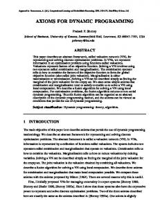
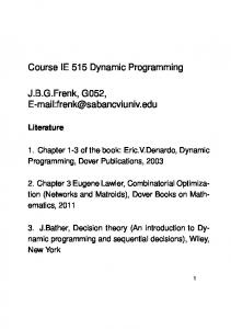
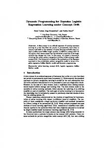
All presented results have been carried out on a Linux machine with 2.33 GHz Intel Core 2Duo CPU E6550 and 2 GB RAM. Our aim was not fast benchmark results, but to explore heuristics for finding decompositions of low boolean-width. TreewidthLIB is an online depository containing a collection of 710 graphs, to be used as a benchmark for the comparison of algorithms computing treewidth. TreewidthLIB provides selected instance graphs, for which computing the treewidth is relevant, originating from applications like probabilistic networks, vertex coloring, frequency assignment and protein structures [5]. We ran our heuristic on the graphs in TreewidthLIB. TreewidthLIB contains 710 graphs. For 482 graphs a tree-width bound is given in TreewidthLIB, and for 426 graphs we give a boolean-width bound using our heuristic. For the comparison we concentrate on the 300 graphs for which we have a bound on both tree-width and boolean-width, but let us first discuss the remaining 410 graphs. Among these 410 graphs, there are 126 having only a boolean-width bound, 182 having only a tree-width bound, and 102 having neither. Among the 182 graphs having only a tree-width bound there are some in a graph format not supported by our implementation, but for the majority of these graphs our heuristic simply timed out already at the greedy initialization stage. Note that for these 182 graphs, if we were given the decomposition of low tree-width k, we could easily have produced a decomposition of boolean-width at most k, using the O(nk 2 ) algorithm which can be deduced from [1]. We now summarize our findings for the 300 graphs having both a tree-width bound and a boolean-width bound. Firstly, the boolean-width bound is always better than the tree-width bound, with the ratio of the tree-width bound divided by the boolean-width bound ranging from 1.15 to 29, with an average of 3.13. Not surprisingly, the ratio increased with higher edge density. In Fig.1 we have plotted this ratio against the edge density of the graphs for a total of 300 graphs. The trend line shows the growth of ratio with edge density. Our heuristic algorithm starts with greedily finding a full decomposition tree giving an Initial Bound on boolean-width and then improves this bound iteratively. In the experiments we kept track of the decrease in the boolean-width over time. In Fig. 2 and Fig. 3 the upper bounds on boolean-width, i.e. the values of boolw(BEST (V )), are shown as they decrease over time, for the two graphs called eil51.tsp (V =51 and E=140) and miles1500 (V=128,E=5198). For the graph eil51.tsp the Initial Bound was 9.1 after less than a second, then at the ’knee’ of the curve before the improvement decays we found a Fast Bound of 6.2 after 4 seconds, and finally the Best Bound of 5.8 was found after 124 seconds. For each graph, we can likewise speak of three bounds: i) the Initial Bound given by the greedy initialization, ii) a Fast Bound found at the ’knee’ of the curve, and iii) the Best Bound found possibly after a long runtime. In Table 1 we summarize results for 8 selected graphs having a good variety of number of vertices V , edge density density, Time in seconds to find Initial Bound, Fast Bound, and Best Bound on boolean-width, its best known treewidth upper bound TWUB, and Ratio=TWUB/BWUB(Best Bound). The graphs are sorted by this Ratio. The miles1500 graph is translated from the Stanford GraphBase. The zeroin.i.1 and mulsol.i.5 graphs originate from the 2nd DIMACS implementation challenge [10] and are generated from a register allocation problem based on real code. The queen8 12 also

35 Graph instances y=143x4−164x3+48x2+1.9x+1.6 30

Ratio=TWUB/BWUB

25

20

15

10

5

0

0

0.1

0.2

0.3

0.4 0.5 0.6 Edge density

0.7

0.8

0.9

1

Fig. 1. Ratio (treewidth divided by boolean-width) versus edge density in all the 300 graphs for which heuristically computed upper bounds are known.

9.5

5.6

9

5.5

8.5

5.4

8

5.3

Boolean−width

Boolean−width

Initial Bound

7.5

7

6.5

Initial Bound

5.2

5.1

5 Fast Bound

Fast Bound

6

4.9

Best Bound

Best Bound 5.5

0

20

40

60 80 Time(sec)

100

120

140

Fig. 2. Improvement of boolean-width upper bound as the local search progresses over time, for the graph eil51.tsp (V=51,E=140)

0

100

200

300 400 Time(sec)

500

600

700

Fig. 3. Improvement of boolean-width upper bound as the local search progresses over time, for the graph miles1500 (V=128,E=5198)

comes from the DIMACS[10] graph coloring problems and is an example of n-queens puzzle. The graph 1awd is from the field of computational biology with each vertex representing a single side chain and each edge representing the existence of a pairwise interaction between the two side chains. The graph celar06-wpp is a frequency assignment instance. The graph BN 28 originates from Bayesian Network from evaluation of probabilistic inference systems at UAI 2006. The graph eil51.tsp is a Delauney triangulation of a traveling salesman problem. Table 1. Results for selected graphs

Graph name miles1500 zeroin.i.1 mulsol.i.5 queen8 12 1awd celar06-wpp BN 28 eil51.tsp

Edge Initial Bound Fast Bound Best Bound V density BWUB Time(s) BWUB Time(s) BWUB Time(s) TWUB Ratio 128 0.64 5.5 32.6 4.9 345.7 4.8 609.6 77 15.85 211 0.19 4.0 74.1 3.8 116.2 3.7 168.0 50 13.51 186 0.23 6.4 55.3 5.4 130.0 4.9 365.2 31 6.25 96 0.30 16.7 3055 16.7 3055 16.7 3055 65 3.91 89 0.27 13.3 67.5 11.1 521.1 10.8 702.9 38 3.52 34 0.28 4.5 0.1 3.2 0.8 3.0 4.8 11 3.37 24 0.18 3.3 0.02 2.3 0.05 2.0 0.3 5 2.50 51 0.11 9.1 0.9 6.2 4.1 5.8 124.6 9 1.55

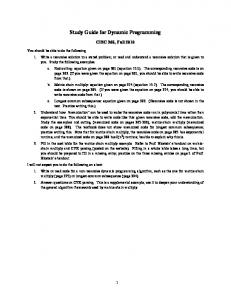
4.1 Small grid graphs We also ran our heuristic on graphs corresponding to the n×n grid. However, for square grids the current implementation of UN(A) is too memory-intensive and we had to limit the size to n ≤ 9. These are sparse graphs having tree-width n and the upper bound we find on boolean-width is below this. See Figure 4. The boolean-width of square n × n grids is a topic we are investigating and our current guess is that the optimal upper bound, holding for all n, is about 0.8 ∗ n. If this is correct, the value computed by the heuristic is close to optimal, which is somewhat interesting as it is our understanding that the heuristics for finding decompositions of low tree-width do not perform well on grid graphs.

5

Conclusion

We presented the first experimental study on computing a notion of width that works also for non-sparse graphs, based on the boolean-width parameter. Experiments with the graphs in TreewidthLIB show the strength of boolean-width versus tree-width, in a practical setting, in particular for graphs of edge density above a certain value. For more examples of real-world graphs of high edge density and high tree-width we could also look beyond the TreewidthLIB library. There are a number of open problems related to boolean-width heuristics and some have already been discussed in subsection 3.3. Firstly, we need a fast heuristic that directly constructs a reasonable upper bound on

9 8

Boolean−width of Grid nxn

7 6 5 4 3 2 1 0

0

1

2

3

4

5

6

7

8

9

n

Fig. 4. Upper-bound on boolean-width, as computed by our heuristic, for the n × n grid, with n ranging from 2 to 9. Tree-width is given by the dotted line x = y.

the boolean-width for any graph, regardless of how big the graph is or what its edge density is. The main issue will be to give a fast heuristic for the computation of a good upper bound on |U N (A)|. Secondly, we need to consider heuristics for computing lower bounds on boolean-width, just as it has been done for tree-width [6]. Thirdly, we should explore pre-processing to simplify the graph instances, again this has been done extensively for tree-width [4]. These problems are of interest since our results indicate that using boolean-width could in the future outperform the use of tree-width in practice for a large class of graphs and problems.

References 1. I. Adler, B. M. Bui-Xuan, Y. Rabinovich, G. Renault, J. A. Telle, and M. Vatshelle. On the boolean-width of a graph: Structure and applications. Proceedings of the 36th International Workshop on Graph-Theoretic Concepts in Computer Science, WG 2010, pages 159–170, 2010. 2. R. Belmonte and M. Vatshelle. Graph classes with structured neighborhoods and algorithmic applications. Proceedings of the 37th International Workshop on Graph-Theoretic Concepts in Computer Science, WG 2011, 2011. see full version www.ii.uib.no/ martinv/Papers/LogBoolw.pdf. 3. Hans L. Bodlaender. A linear time algorithm for finding tree-decompositions of small treewidth. SIAM Journal on Computing, 25:1305–1317, 1996. 4. Hans L. Bodlaender. Treewidth: Characterizations, applications, and computations. In Fedor V. Fomin, editor, Proceedings of the 32nd International Workshop on Graph-Theoretic Concepts in Computer Science, WG 2006, pages 1 – 14. Springer Verlag, LNCS, vol. 4271, 2006. 5. Hans L. Bodlaender and Arie M. C. A. Koster. Treewidth computations I. Upper bounds. Information and Computation, 208:259–275, 2010. 6. Hans L. Bodlaender and Arie M. C. A. Koster. Treewidth computations II. lower bounds. Technical Report UU-CS-2010-022, Department of Information and Computing Sciences, Utrecht University, Utrecht, the Netherlands, 2010. Accepted for publication in Information and Computation.

7. A. Brandstadt. personal communication. 8. B. M. Bui-Xuan, J. A. Telle, and M. Vatshelle. Boolean-width of graphs (to appear). Theoretical Computer Science, 2011. see full version www.ii.uib.no/ telle/bib/listofpub/BTV11.pdf. 9. Hubie Chen. Quantified constraint satisfaction and bounded treewidth. In Ramon L´opez de M´antaras and Lorenza Saitta, editors, Proceedings of the 17th European Conference on Artificial Intelligence, ECAI 2004, pages 161–165, 2004. 10. The second DIMACS implementation challenge: NP-Hard Problems: Maximum Clique, Graph Coloring, and Satisfiability. See http://dimacs.rutgers.edu/Challenges/, 1992–1993. 11. Georg Gottlob, Nicola Leone, and Francesco Scarcello. A comparison of structural CSP decomposition methods. Acta Informatica, 124:243–282, 2000. 12. Illya V. Hicks, Arie M. C. A. Koster, and Elif Koloto˘glu. Branch and tree decomposition techniques for discrete optimization. In J. Cole Smith, editor, TutORials 2005, INFORMS Tutorials in Operations Research Series, chapter 1, pages 1–29. INFORMS Annual Meeting, 2005. 13. P. Hlinˇen´y and S. Oum. Finding branch-decomposition and rank-decomposition. SIAM Journal on Computing, 38:1012–1032, 2008. 14. K. H. Kim. Boolean matrix theory and its applications. 1982. Marcel Dekker. 15. S. J. Lauritzen and D. J. Spiegelhalter. Local computations with probabilities on graphical structures and their application to expert systems. The Journal of the Royal Statistical Society. Series B (Methodological), 50:157–224, 1988. 16. Arnold Overwijk, Eelko Penninkx, and Hans L. Bodlaender. A local search algorithm for branchwidth. Proceedings of the 37th Conference on Current Trends in Theory and Practive of Computer Science, SOFSEM 2011, pages 444–454, 2011. 17. Hein R¨ohrig. Tree decomposition: A feasibility study. Master’s thesis, Max-Planck-Institut f¨ur Informatik, Saarbr¨ucken, Germany, 1998. 18. Y. Song, C. Liu, R. Malmberg, F. Pan, and L. Cai. Tree decomposition based fast search of RNA structures including pseudoknots in genomes. In Proceedings of the 2005 IEEE Computational Systems Bioinformatics Conference, CSB’05, pages 223–234, 2005. 19. Treewidthlib. http://www.cs.uu.nl/people/hansb/treewidthlib, 2004– . . . . 20. Johan M. M. van Rooij, Hans L. Bodlaender, and Peter Rossmanith. Dynamic programming on tree decompositions using generalised fast subset convolution. In Amos Fiat and Peter Sanders, editors, Proceedings of the 17th Annual European Symposium on Algorithms, ESA 2009, pages 566–577. Springer Verlag, Lecture Notes in Computer Science, vol. 5757, 2009. 21. Jizhen Zhao, Dongsheng Che, and Liming Cai. Comparative pathway annotation with protein-DNA interaction and operon information via graph tree decomposition. In Proceedings of Pacific Symposium on Biocomputing, PSB 2007, volume 12, pages 496–507, 2007. 22. Jizhen Zhao, Russell L. Malmberg, and Liming Cai. Rapid ab initio prediction of RNA pseudoknots via graph tree decomposition. Journal of Mathematical Biology, 56(1–2):145– 159, 2008.