ABSTRACT. Modern embedded system execute a single application or a class of applications repeatedly. A new emerging methodology of designing.
Finding Optimal L1 Cache Configuration for Embedded Systems Andhi Janapsatya†, Aleksandar Ignjatovic´ †‡, Sri Parameswaran†‡ †School of Computer Science and Engineering, The University of New South Wales
Sydney, NSW 2052, Australia
‡NICTA, The University of New South Wales
Sydney, NSW 2052, Australia {andhij,sridevan,ignjat}@cse.unsw.edu.au
g721enc
1000
00
0 00
00
00 00 10
10
00
00
0 00 10
00 10
0
Total Cache Miss (hundreds)
10
Today, cache memory is an integral component of mid to high end processor based embedded systems. The inclusion of cache significantly improves system performance and reduces energy consumption. Current processor design methodologies rely on reserving large enough chip area for caches while conforming with area, performance, and energy cost constraints. Recent application specific processor design platforms (such as the Tensilica’s Xtensa platform [1]) allows a cache to be customized for the processor. This allows a design which can meet tighter energy consumption, performance, and cost constraints. In existing low power processors, cache memory is known to consume a large portion of the on-chip energy. For example, in [2] Montanaro et al. report that cache consumes up to 43% of the total energy of a processor. In embedded systems where a single application or a class of applications are repeatedly executed on a processor, the memory hierarchy could be customized such that an optimal configuration is achieved. The right choice of cache configuration for a given application could have a significant impact on overall performance and energy consumption. Choosing the correct cache configuration for an embedded system is crucial in reducing energy consumption and improving performance. To find the correct configuration the hit and miss rates must be evaluated, and the resulting energy consumption and execution times must be accurately estimated. Estimating the hit and miss rates (for a particular application with sample input data) is fairly easy using tools such as Dinero IV [7], but enormously time consuming to do so for various cache sizes, associativities and line sizes. The resulting energy consumption and execution times are difficult to examine due to the non uniform nature of memory, where the first memory access takes far greater time compared to subsequent accesses (which are sequential to the first access). Energy and access times are further complicated by differing cache configurations consuming energy at different rates and taking differing amounts of time to access. Our research results demonstrate that low miss rates do not necessarily mean a faster execution time. Figure 1 shows the effect of different cache configurations have on the number of total cache misses and the total execution time for the G721 encode application. The graph in Figure 1 shows that higher total cache miss rates can possibly provide the fastest execution time. This is due to large or more
10
1. Introduction
10
100 1
Modern embedded system execute a single application or a class of applications repeatedly. A new emerging methodology of designing embedded system utilizes configurable processors where the cache size, associativity, and line size can be chosen by the designer. In this paper, a method is given to rapidly find the L1 cache miss rate of an application. An energy model and an execution time model are developed to find the best cache configuration for the given embedded application. Using benchmarks from Mediabench, we find that our method is on average 45 times faster to explore the design space, compared to Dinero IV while still having 100% accuracy.
10000
Total Execution Time (ms)
ABSTRACT
Figure 1: Total Cache miss vs. Total Execution Time complex (higher associativity) caches having significantly longer access times. Existing methodologies for cache miss rate estimation, use heuristics to search through the cache parameter design space [3, 4, 5, 6]. Other existing cache miss rates estimation tools, such as Dinero IV [7] can accurately determine the cache miss rate for a single cache configuration. To use Dinero IV to estimate cache miss rate for a number of cache configurations means that a large program trace needs to be repeatedly read and evaluated which is time consuming. In this paper, we present a methodology to rapidly and accurately explore the cache design space by: estimating cache miss rates for many different cache configurations simultaneously; and investigate the effect of different cache configurations on the energy and performance of a system. The method performs simultaneous evaluation of multiple cache configurations by reading a program trace just once. Simultaneous evaluation can be rapidly performed by taking advantage of the high correlation between cache behavior of different cache configurations. The idea of utilizing correlation in cache behavior comes from the following observations: one, given two caches with the same associativity using the Least Recently Used (LRU) replacement policy, whenever a cache hit occurs, all caches that have larger set sizes will also guarantee a cache hit; two, a hit on a setassociative cache means a cache hit is guarantee on all caches with larger associativity (Explained in greater detail in Section 3). These observations were also described [8] and [9]. Gecsei et al. in [8] introduce the “stack algorithm” for finding the exact frequency of accesses to each level in a memory hierarchy system. In [9], Hill and Smith analyze the effect of different cache associativity on cache miss rates. The benefit of our method is a quick exploration of different cache parameters from a single read of a large program trace. This will then allow an embedded system to be tested with multiple input sets and with multiple architectures, where it may not be possible to store the large program traces. The rest of this paper is structured as follow, Section 2 presents existing cache exploration methodologies; Section 3 presents our cache parameters exploration space methodology; Section 4 describes the performance and energy model for the system architecture consid-
1010
ered in this work; Section 5 describes the experimental setup and discusses the results; and Section 6 concludes the paper. Cache simulation is required for tuning cache parameters to ensure maximal performance and minimal energy consumption. In the past, various methodologies have been researched for cache simulation. These cache simulation methodologies can be divided into two classes: one, estimation techniques, and the other, exact simulation. Cache estimation techniques use heuristics to predict the cache misses for multiple cache configurations. Pieper et al. in [3] developed a metric to represent cache behavior independently of the cache structure. Their metric based result is within 20% accuracy of a uniprocessor trace-based simulation and can be applied for estimating multiprocessor architectures. In [4], Fornaciari proposed a heuristic method for configuration of cache architecture without exhaustive analysis of the space of parameters. Their analysis looked at the sensitivity of individual cache parameters on the energy delay product. Maximum error is less than 10%. Ghosh et al. described a method to generate and solve a cache miss equations (CME) to represent the cache behavior [5]. In [6], Vera et al. proposed a fast and accurate method to solve the cache miss equation (CME). For exact cache simulation techniques, there exists a tool called Dinero IV [7]. Dinero IV is a single processor cache simulation tool developed by Jan Edler and Mark Hill. Its purpose is to estimate the number of cache misses given a cache configuration; its features include simulating separate or combined instruction and data caches, and simulating multiple levels of cache. For simulating multiple cache configurations, exact cache simulation techniques rely on exploiting the inclusion property of caches. Inclusion means that given two cache configuration, Cache C2 ⊂ Cache C1 if all the content of Cache C2 is a subset of the content of Cache C1 . In 1970, Gecsei et al. [8] introduced the ‘Stack’ algorithm for performing simulation of multiple levels of storage systems. In 1989, Hill in [9] investigated the effects of associativity of caches. They briefly described the methodology of forest simulation for quick simulation of alternate direct-mapped caches. They also introduced the all-associative methodology for simulating alternate direct-mapped, set-associative, and fully-associative caches based on the ‘Stack’ algorithm. The space complexity of the all-associativity simulation is O(Nunique ), where Nunique is the number of unique blocks referenced in an address trace. In their experiment, they showed that to simulate alternate direct-mapped caches, the forest simulation method is faster than the all-associative simulation. Sugumar et al., introduced a cache simulation methodology by using a binomial trees [10] to improve the method described in [9]. The time complexity of their algorithm for searching procedure is O((log2 (N) + 1) × A) and the time complexity for maintaining the binomial tree is O((log2 (N) + 1) × A), where N is the size of the cache and A is the associativity of the cache. Li in [11] then extends the work in [10] by introducing a method to compress the program trace for reducing the cache simulation time. Other existing exact cache simulation methodologies uses parallel processing units and/or multiprocessor systems. Nicol in [12] presented a parallel methodology to simulate cache using SIMD and MIMD hardware units. Heidelberger in [13] presented a method of to analyze a cache trace using a parallel processor system. They split long traces into several shorter traces, and the shorter traces are then executed on parallel independent processors. The sum of the individual results are not accurate, but by executing a re-simulation phase, it is possible to accurately count the exact number of cache misses. Our simulation methodology was created as a forest simulation data structure. Our methodology extends the idea of forest simulation described in [9]. The space complexity of our methodology is fixed depending on the number of cache configurations to be evaluated. The required space of our cache simulation method is larger than the
101(1)
101(0)
2. Related Work 10(00)
1(000)
10(01)
10(10)
1(100) 1(010)
1(110)
1(001)
Cache Size = 2
10(11)
1(101) 1(011)
Cache Size = 4
1(111) Cache Size = 8
Figure 2: The cache tree data structure. space needed for the all-associativity simulation described in [9] and the binomial tree simulation described in [10]. The time complexity for searching our data structure is O((log2 (N)+1)×A), and the time complexity for updating the data structure is O(log2 (N) + 1). This is faster compared to the method described in [10]. Other research looked at the use of heuristics for predicting cache behavior. Ghosh et al, in [14] presented an algorithm for simulating cache parameters and finding cache configurations that guaranteed cache miss rates lower than a desired cache miss rate. Their space complexity is in the order of the size of the trace file.
2.1 Our Contribution • For the first time a methodology is proposed which allows an L1 cache to be chosen for an Application Specific Instruction Set Processor (ASIP) based upon the energy consumption and execution time. • We also propose a modified forest algorithm based on a simplified data structure, for fast and accurate simulation of the cache. The time taken by the algorithm for both simulation and updating of the data structure is considerably quicker than previous methods. In addition, this method allows parallelization.
3. Cache Parameters Exploration Methodology A cache configuration is dependent on the cache parameters: cache size N, cache associativity A, and cache line size L. The cache size refers to the total number of bits that can be stored in the cache. The cache associativity refers to the number of ways a data can be stored within the same address of the cache. For a direct-mapped cache (A = 1), each datum has a single location where it can be stored within the cache. The total cache size divided by associativity of the cache is called the cache set size, M = N/A. In our simulations we will consider cache configurations with the cache set in the range from 2mmin to 2mmax , where mmin and mmax refer to the number of address bits needed to address 2mmin and 2mmax locations. We perform design space exploration on the cache parameters by accurately and efficiently simulating the number of cache misses that would occur for a given collection of cache configurations. We optimize the run time of our cache simulation by replacing multiple readings of large program traces with a single reading and simulating multiple cache configurations simultaneously. This is possible due to the following observations. First, assume that two cache configurations have the same associativity and the same cache line size but that one cache is twice the size of the other cache. In this case if a cache hit occurs on the smaller size cache, a cache hit will also occur on the larger cache size. This is illustrated in Figure 2. For a memory address request of ‘1010’, cache location pointed to by the address ‘1010’ can be found on the cache locations shown with the dotted line branches in Figure 2. The numbers inside the parentheses shown in Figure 2 indicate the cache address for that location. From the figure, it can be seen that the entries within cache size = 2 are a subset of the entries within cache size = 4, and the entries within cache size = 4 are a subset of the entries within cache size = 8. The second observation is that if a cache miss occurs for a cache of size N, associativity A, and of cache set size M, then for all other cache configurations with the same cache set size M and associativity larger than A, a cache hit will also occur. Hence, evaluation for all values larger than A is not required to determine the number of cache
Array
Forest
Linked List
Figure 3: The cache simulation data structure. Cache Assoc. = 1
Cache Assoc. = 2
Cache Assoc. = 4
Most recently used element in the cache.
Least Recently Used element in the cache.
Figure 4: The linked list data structure. misses for such configurations. This observation is also known as ‘inclusion’ [8].
3.1 Cache Simulation Methodology Based on the two observations described above, we designed and implemented the following procedure for simultaneous simulation of multiple cache configurations using a single read of the program trace. We created an array of cache miss counters to record the cumulative cache misses that occur with different cache configurations. The size of this array is dependent on the number of cache configurations to be simulated and the array is indexed using cache configuration parameters. To simulate the cache, we created a collection of forest data structures as follows. Each forest corresponds to a collection of cache configurations that have the same cache line size. Each tree in such a forest is used as a convenient data structure to store pointers to locations in cache sets for caches of different sizes. An array of size equal to minimum cache set size 2mmin is created to store addresses of such trees; note that mmin bits are required to address 2mmin such locations of the array. The kth level of the tree corresponds to the cache configuration with the cache set size 2k+mmin . Each node in the tree corresponds to a cache location and points to a linked list. Elements in this list correspond to cache ways, and will be used to store the tag address, the valid bit, and the pointer to the next element. The total number of elements in each linked list corresponds to the largest associativity of the family of cache configurations considered. The head element of the linked list corresponds to the most recently used data in the cache; the tail corresponds to the least recently used data. The linked list is illustrated in Figure 4, and the whole data structure is illustrated in Figure 3. Searches of each linked list on different nodes of the tree are independent of each other; this property allows parallelization to optimize the simulation procedure. To simulate different cache line sizes, we replicate the forest for each cache line size parameter that need to be simulated. For the sake of explanation, we first assume that the cache line size is fixed to one byte; as this assumption does not change the nature of the algorithm. The cache simulation methodology is shown in Figure 5 and illustrated in Figure 6. The methodology takes its input from the program trace. For each address x read from the program trace, we use the least significant mmin bits of the address x to locate in the array the pointer to the appropriate tree. For each cache set size of the form 2k+mmin , thus ranging in powers of two from 2mmin to 2mmax we take the next k bits of the memory address and use these bits to find the node in the tree that corresponds to the cache set location in the cache of this size (i.e., 2k+mmin ). This is done by traversing down the
For each address x from the trace { Use the least significant mmin bits of the address x to locate in the array, the pointer to the corresponding tree, and go to the root of the tree. For k = 0 to (mmax − mmin ) { // k corresponds to the level of the tree; // the total cache set size is 2k+mmin Go to the head of the linked list pointed by this node of the tree Search linked list to find the tag entry that is equal to the tag of the address x. If a cache hit occurs in an element s of the linked list{ Increment cache miss counters for all cache configuration with cache set size equal to 2k+mmin and lower associativity than s. Move element s to be the head element of the linked list. } else { Increment cache miss counter for all cache configuration with cache set equal to 2k+mmin Replace entry in the tail element of the linked list with the current tag address. Move this tail element to become the head element of the linked list. } Increment the value of k. Step down the tree according to the value of the bit k + mmin taking the left child if this bit is 0 else take the right child. } Scan the next address x + 1 from the trace. }
Figure 5: Cache Simulation Procedure m tag address
max
min
m
cache addr.
Figure 6: Cache Simulation Procedure. tree depending on the mmin to mmin + k bits of the address to choose whether to traverse the left branch or the right branch. The node has a pointer to the head element in the linked list that corresponds to the multiple way associativity of this cache set location. The remaining bits of the address x form the tag address that is to be searched for in the linked list. If the tag is found at position s, this indicates that a cache hit would occur in all s-way or higher-way associative caches. If this happens, the sth element of the list is moved to the head of the list. In this case, all cache miss counters for caches with the same cache set size and associativity less than s are incremented. If the tag is not found, the tag in the tail element is replaced by the new tag, and this tail element is moved to the head of the list. In such a case, cache miss counters for caches with the same cache set size and any values of associativity are incremented. This is illustrated for a 4-way set-associative cache in Figure 4. If the tag comparison results in a hit with the second element in the linked list, then this indicates that a cache hit would occur in the 4-way set-associative cache and the 2-way set-associative cache. A cache miss would occur in the direct mapped cache, hence it is not necessary to continue the search until the tail element. The second element is then moved to be the head element to conform with the Least Recently Used (LRU) replacement policy. The procedure continues by traversing down the trees to find the linked list corresponding to the larger cache set size. The procedure for tag comparison and updating the associativity replacement policy is then repeated. An example is shown in Figure 2, once the cache estimation for the level cache size = 2 is completed, the algorithm will look at the least significant bit of the current tag part of the address which will make up the most significant bit of the cache address for the cache size = 4 tree level to determine whether to traverse the left or right branch. In Figure 2, the dotted line indicates the traversing path given the address ‘1010’. The algorithm then continues by using the replicated forest data
CPU
I-Cache
Application cjpeg djpeg pegwitenc pegwitdec epic unepic g721enc g721dec mpeg2enc mpeg2dec
D-Cache
DRAM (main memory)
Figure 7: System Architecture structures for simulating the different cache line sizes. Different parts of the current address are used for locating the appropriate tree data structure.
3.2 Efficiency of The Methodology With the implementation described above, we can limit the search space for all the different cache configurations and reduce the time taken to estimate cache misses by increasing the space requirements. Each linked list entry is used to store the tag address (32 bits), a valid bit (1 bit), and a pointer to the next element in the linked list (32 bits). In total, each linked list entry needs to keep 65 bits of data. Each node in the tree needs to store pointers to the head element of the linked list (32 bits), a pointer to the left branch (32 bits), and a pointer to the right branch (32 bits); giving a total of 96 bits per node. For each cache way, a linked list entry needs to be kept, this gives a total size of listsize = A × 65bits. The number of nodes created is dependent on the number of cache sets, cache line size, and cache size range. The number of nodes is calculated by nodesize = (2mmax − 2mmin ) × (log2 (L) + 1) × 96 bits. Space complexity is calculated by summing all the space needed for each node and each linked list entry. In terms of space, our data structure is optimal for storing all the necessary parameters with exception of the redundancy of the content of the linked lists. However, the space requirement is fully manageable by standard desktop computers. For the work described in this paper, we simulated cache sizes ranging from 512 bytes up to 2M bytes, cache associativity of 1 up to 32, and cache line size of 8 bytes up to 256 bytes. In total, we have simulated 268 cache configurations requiring 9.3 megabytes. This reasonable redundancy simplifies the maintenance of the data structure and the associated algorithms.
4. System Energy and Performance Model To facilitate the design space exploration steps, we created crude performance and energy models for the system. The model of the embedded system architecture consisted of a processor with an instruction cache, a data cache, and embedded DRAM as main memory. The data cache uses a write-through strategy. The system architecture is illustrated in Figure. 7. The equation for calculating the system’s total execution time is given by: Exectime =Icacheaccess × Icacheaccess time + Icachemiss × DRAMaccess time + 1 + DRAMbandwidth Dcacheaccess × Dcacheaccess time + Dcachemiss × DRAMaccess time + 1 Dcachemiss × Dcachelinesize × DRAMbandwidth
Icachemiss × Icachelinesize ×
(1)
where, • Icacheaccess and Dcacheaccess is the total number of memory accesses to the instruction and data cache, respectively. • Icacheaccess time and Dcacheaccess time is the access time of the instruction and data cache, respectively.
Total Execution Time (sec) Trace size Dinero IV Our methodology ratio 15531057 1592 41 38.83 4616784 363 20 18.15 33070433 2831 136 20.82 18903066 1642 70 23.46 52801084 4017 30 133.90 6746679 512 6 85.33 3.15E+08 (7.5 hr) 26990 (26.5 min) 1595 16.92 3.03E+08 (7 hr) 25132 (25 min) 1503 16.72 1.13E+09 (25.2 hr) 90431 (53 min) 3186 28.38 35398584 3377 49 68.92 Average 45.14
Table 1: Total execution time comparison of our methodology with Dinero IV. • Icachemiss and Dcachemiss is the total number of cache misses for the instruction and data cache, respectively. • Icachelinesize and Dcachelinesize is the cache line size of the instruction and data cache, respectively. • DRAMaccess time is the DRAM latency time. • DRAMbandwidth is the bandwidth of the DRAM. There exists six components in the system’s execution time shown in equation 1. The first and fourth terms Icacheaccess ×Icacheaccess time and Dcacheaccess × Dcacheaccess time are for calculating the amount of time taken for the processor to access the instruction cache or the data cache. The second and fifth terms Icachemiss × DRAMaccess time and Dcachemiss × DRAMaccess time calculate the amount of time required for the DRAM to respond to each cache miss. The third and sixth terms Icachemiss ×Icachelinesize × DRAM1bandwidth and Dcachemiss × Dcachelinesize × DRAM1bandwidth calculates the amount of time taken to fill a cache line on each cache miss. In our execution time model, we assume that all data cache misses will cause a pipeline stall, and we ignore the bus communication time cost. As the bus communication time is expected to be similar to other systems, ignoring this will not adversely affect the final results. Energy equation of the system is given by the following equation: Energytotal =Exectime ×CPU power + Icacheaccess × Icacheaccess energy + Dcacheaccess × Dcacheaccess energy + Icachemiss × Icacheaccess energy × Icachelinesize + Dcachemiss × Dcacheaccess energy × Dcachelinesize + Icachemiss × DRAMaccess power × 1 )+ (DRAMaccess time + Icachelinesize × DRAMbandwidth Dcachemiss × DRAMaccess power × 1 ) (DRAMaccess time + Dcachelinesize × DRAMbandwidth (2) where, • CPU power is the total processor power excluding the instruction and data cache power. • Icacheaccess energy and Dcacheaccess energy is the instruction cache and data cache access energy, respectively. • Dcacheaccess
power
is the active power consumed by the DRAM.
There exist seven components in the energy equation 2. The first term Exectime ×CPU power calculates the processor energy given that execution time takes Exectime amount of time. The second and third
Processor Energy Embedded DRAM energy Latency Bandwidth
168mW @ 100MHz @100MHZ 19.5mW 19.5 ns 50MB/sec
5.1 Result Analysis
Table 2: System Specification 1600 Total ExecutionTime (min)
1400
DineroIV Our Estimation Tool
1200 1000 800 600 400 200 0 1
10
100 Trace size (millions)
1000
10000
Figure 8: Total execution time compared to increasing program trace size terms, Icacheaccess × Icacheaccess energy and Dcacheaccess × Dcacheaccess energy calculate the amount of energy consumed by the instruction and data cache, respectively. The fourth and fifth terms, Icachemiss × Icacheaccess energy × Icachelinesize and Dcachemiss × Dcacheaccess energy × Dcachelinesize calculate the energy cost of writing to cache for each cache miss. The sixth and seventh terms, Icachemiss × DRAMaccess energy × (DRAMaccess time + Icachelinesize × DRAMbandwidth ) and Dcachemiss × DRAMaccess energy × (DRAMaccess time +Dcachelinesize ×DRAMbandwidth ) calculate the energy cost of the DRAM to service all the cache misses. The fourth, fifth, sixth, and seventh terms vary depending on the cache line size, as larger line size means more data need to be read from the main memory and written into the respective caches. Units for time variables in the equations are in seconds, bandwidth is in bytes/sec., cache line size is in bytes, power variable is in Watts, and energy unit is in Joules.
5. Experimental Procedure and Results We compiled and simulated programs from Mediabench [15] with SimpleScalar/PISA 3.0d [16]. Program traces were generated by SimpleScalar and fed into both Dinero IV[7] and our estimation tool. Our results were completely consistent with the ones produced by Dinero IV. Our estimation tool is written in C and compiled with GNU/GCC version 3.4.3 build 20050227 with -O1 optimization. Simulations were performed on a dual Opteron64 2GHz machine with 2GBytes of memory. We simulated 268 different cache configurations, with cache sizes ranging from 512 Bytes up to 2M bytes, cache associativity ranging from 1 up to 32, and cache block sizes ranging from 8 bytes per cache line up to 256 bytes per cache line. Table 1 shows the execution time comparison of executing Dinero IV multiple times with different cache configurations and execution of our estimation tool once. Column 1 in Table 1 shows the application name, column 2 shows the trace size of the benchmark, column 3 shows the total time taken for executing Dinero IV multiple times, column 4 shows the execution time of our estimation tool, and column 5 shows the ratio of time savings of our tool when compared to executing Dinero IV multiple times. The trace size shown in Column 2 in Table 1 only shows the size of the instruction memory access trace. From column 5 in Table 1, it can be observed that, on average, our tool is approximately 45 times faster than Dinero IV. Plotting the total execution time versus the size of the trace in Figure 8 shows that as the trace size grows exponentially, our methodology shows a linear increase in total execution time required while Dinero IV shows an exponential increase in the time required.
To analyze the effect of cache miss rates on system’s performance and energy consumption, we utilized cache models from CACTI [17] for the cache access time and cache access energy. Processor energy is taken from [2]. The main memory model is taken from the embedded DRAM described in [18]. The processor and memory specification is described in Table 2. System total execution time and its energy consumption is calculated using equation 1 and equation 2, respectively. In Figure 9, We plot the number of cache misses versus the total energy consumption for different cache configurations. The plot for cache misses versus execution time for g721enc application was shown in Figure 1. The three plots in Figure 9 show the same plot with different coloring to pick out the effect of differing cache line sizes, cache associativity, and cache sizes on the energy consumption. Figure 9(b) highlights the effect of different cache line size on the total energy consumption. Figure 9(a) highlights the effect of changing associativity on the total energy consumption. Figure 9(c) highlights the effect of varying cache sizes on the total energy consumption. Due to space constraints, we are unable to show the cache miss versus total execution time graphs with different coloring to highlight the effect of cache associativity, cache line size, and cache size on the total execution time.
5.2 Model Validation We validate the energy model of the processor by comparing with output results of Wattch [19]. The mediabench applications were executed in Wattch and the total energy results is plotted against the total cache miss number. Figure 10 shows the total energy versus the total cache miss number for g721enc application with energy figures obtained from Wattch output. Comparing the energy versus cache miss number graphs in Figure 10 and in Figure 9(c) show that energy results from Wattch and from equation 2 display similar patterns. As cache size gets larger, the cache miss number decreases and the energy consumption decreases; but when the cache size reaches a certain size, the energy consumption starts to increase due to compulsory misses. It should be noted that simulation time for the 268 cache configurations with Wattch took 2.5 days. The energy values obtained from Wattch simulation has a unit of Watts.cycle and the energy values should not be compared directly against the energy values obtained from Equation 2. The energy graphs obtained using the Equation 2 and from Wattch is not an exact copy of each other. This error is due to several reasons, such as, the different processor parameters of the two processors and the inaccuracy of the simplescalar model (Wattch is built on top of Simplescalar) for reporting cache misses. In addition, it is also known that processor energy calculation using processor model derived from simplescalar is inaccurate; for example, simplescalar modeled the issue queue, reorder buffer, and the physical register file as a unified structure called Register Update Unit (RUU), unlike in real implementations where the number of entries and the number of ports in all these components are quite disparate [20]. We also performed simulation with Wattch for the remaining Mediabench benchmarks and obtained similar energy graph results in comparison to energy graph obtain from using Equation 2. Due to space constraints, we are unable to include the energy graphs obtained with Wattch for all other benchmarks.
5.3 Design Space Exploration Looking at the Pareto optimal points in the three plots (Figure 9), it can be concluded that for g721enc application a 16K bytes directmapped cache with line size of 16 bytes would be the best cache configuration in terms of lowest energy consumption. For design space exploration purposes, the best cache configuration based on performance or energy consumption can then be chosen from the performance plots and the energy plots. Best choices of cache configurations for the Mediabench benchmark is shown in Table 3. For g721enc application, it can be seen in Table 3 that for best performance a 16K bytes direct-mapped cache with line size of 256
cjpeg djpeg pegwitenc pegwitdec epic unepic g721enc g721dec mpeg2dec
10000 asso 1 asso 2 asso 4 asso 8 asso 16 asso 32
Total Energy (mJ)
Application
Cache configuration corresponding to Best Performance Lowest energy consumption Cache Cache Cache Cache Cache Cache size Assoc. line size size Assoc. line size 16384 1 256 16384 1 16 8192 1 128 8192 1 16 16384 1 128 16384 1 16 8192 1 128 8192 1 8 8192 1 128 8192 1 32 8192 1 128 4096 1 32 16384 1 256 16384 1 32 16384 1 16 8192 1 64 4096 1 64 4096 1 16
1000
100 1.E+02
Table 3: Best cache configuration choice in terms of performance or energy consumption.
6. Conclusions In this paper, we presented a cache selection method for configurable processors. This method uses a cache simulation procedure to perform fast and accurate simulation of multiple cache configurations simultaneously using a single reading of a program trace. Our method is 45 times faster compared to existing methods of cache simulation. Fast and accurate cache miss calculations allow rapid design space exploration of optimal cache parameters for desired performance and/or energy consumption.
1.E+05
1.E+06
1.E+07
1.E+08
1.E+09
(a) Energy comparison for different cache associativity 10000
block 1 block2 block4 block8 block16 block32
1000
100 1.E+02 1.E+03 1.E+04 1.E+05 1.E+06 1.E+07 1.E+08 1.E+09 Cache Misses
7. References
(b) Energy comparison for different cache line size
Total Energy (mJ)
10000
512 1024 2048 4096 8192 16384 32768 65536 131072 > 131072
1000
100 1.E+02 1.E+03 1.E+04 1.E+05 1.E+06 1.E+07 1.E+08 1.E+09 Cache Misses
(c) Energy comparison for different cache size Figure 9: Total energy consumption compared to cache miss number
1.E+13 size=512 1024 2048 4096 8192 16384 32768 65536 131072 >131072
Total Energy (Watts. cycle)
[1] Xtensa Processor, http://www.tensilica.com. [2] J. Montanaro et al., “A 160MHz, 32b, 0.5W CMOS RISC microprocessor,” JSSC, vol.31(11), pp. 1703-1712, 1996. [3] J. J. Pieper et.al., “High level Cache Simulation for Heterogeneous Multiprocessors,” DAC, 2004. [4] W. Fornaciari et.al., “A Design Framework to Efficiently Explore Energy-Delay Tradeoffs,” CODES, 2001. [5] S. Ghosh et.al., “Cache Miss Equations: A Compiler Framework for Analyzing and Tuning Memory Behavior,” TOPLAS, 1999. [6] X. Vera et.al., “A Fast and Accurate Framework to Analyze and Optimize Cache Memory Behavior,” TOPLAS, 2004. [7] J. Edler and M. D. Hill, “Dinero IV Trace-Driven Uniprocessor Cache Simulator,” http://www.cs.wisc.edu/˜markhill/DineroIV/. [8] R. L. Mattson et.al., “Evaluation Techniques for Storage Hierarchies,” IBM System Journal, vol.9, no.2, pp. 78-117, 1970. [9] M. D. Hill and A. J. Smith, “Evaluating Associativity in CPU Caches,” IEEE Transactions on Computer, 1989. [10] R. A. Sugumar et.al., “Set-Associative Cache Simulation Using generalized Binomial Trees,” ACM Transactions on computer Systems, vol. 13, No. 1, 1995. [11] X. Li et.al., “Design Space Exploration of Caches Using Compressed Traces,” ICS, 2004. [12] D. Nicol and E. Carr, “Empirical Study of Parallel Trace-Driven LRU Cache Simulator, ACM SIGSIM Simulation Digest, Proceedings of the ninth workshop on Parallel and distributed simulation, 1995. [13] P. Heidelberger and H. S. Stone, “Parallel Trace-Driven Cache Simulation by Time Partitioning,” Winter Simulation Conference, 1990. [14] A. Ghosh and T. Givargis, “Analytical Design Space Exploration of Caches for Embedded Systems,” DATE, 2003. [15] C. Lee et.al., “MediaBench: A Tool for Evaluating Multimedia and Communications Systems,” IEEE MICRO 30, 1997. [16] D. C. Burger and T. M. Austin, “The SimpleScalar tool-set, Version 2.0,” Technical Report 1342, Department of Computer Science, UW, June, 1997. [17] P. Shivakumar and N. P. Jouppi, “Cacti 3.0: An Integrated Cache Timing, Power, and Area Model,” Technical Report 2001/2, Compaq Computer Corporation, August, 2001. 2001. [18] K. Hardee et.al., “A 0.6V 205MHz 19.5ns tRC 16Mb Embedded DRAM,” ISSCC, 2004. [19] D. Brooks et.al., “Wattch: A Framework for Architectural-Level Power Analysis and Optimizations,” ISCA, 2000. [20] D. Ponomarev, G. Kucuk, and K. Ghose, “AccuPower: An Accurate Power Estimation Tools for Superscalar Microprocessors,” DATE, 2002.
1.E+04
Cache Misses
Total Energy (mJ)
bytes should be used. This indicates that the lowest energy consuming cache configurations does not translate to the fastest execution time.
1.E+03
1.E+12
1.E+11
1.E+10 1
10
100
1000
10000
100000
Total Cache Misses (Thousands)
Figure 10: Total energy consumption of g721enc application measured using Wattch.