1
FINDING OPTIMAL PORTFOLIOS WITH CONSTRAINTS ON VALUE AT RISK Alexei A. Gaivoronski∗ and Georg Pflug∗∗ ∗
Department of Industrial Economics and Technology Management NTNU - Norwegian University of Science and Technology Alfred Getz vei 1, N-7049 Trondheim, Norway
[email protected] ∗∗ Department of Statistics University of Vienna Universitaetsstrasse 5 A-1010 Vienna, Austria
[email protected]
Abstract Value at risk is an important measure of extent to which a given portfolio is subject to different kinds of risk present in financial markets. Considerable amount of research was dedicated during recent years to development of acceptable methods for evaluation of this risk measure. In this paper we go beyond estimation of value at risk and address the following questions. - Suppose that a boundary for acceptable value at risk is fixed. How to find a portfolio among given set of securities which would provide the maximal yield and at the same time satisfy the constraints on value at risk; - Suppose that the market conditions are changing. How to obtain a portfolio rebalancing strategy which would keep portfolio within given boundary on value at risk and maximize in some sense the yield of resulting sequence of portfolios. In order to solve these problems we adapt and further develop algorithmic tools which have their origin in stochastic optimization and were considered recently in machine learning.
1 Introduction Value at Risk (VAR) is an important measure of exposure of a given portfolio of securities to different kinds of risk inherent in financial environment. By now, it became a tool for risk management in financial industry [1] and part of industrial regulatory mechanisms [2]. Considerable amount of research was dedicated recently to development of methods of risk management based on Value at Risk [3, 11, 12, 13, 18]. This literature is dedicated mainly to efficient techniques for computing VAR of a given portfolio. In this paper we combine the notion of VAR with portfolio optimality. More precisely, we seek to define portfolio which produces maximal yield and at the same time satisfies constraints on Value at Risk. Our aim is to develop a theory similar to Markovitz theory for optimal meanvariance portfolios and provide algorithmic tools for computing such portfolios. Our emphasis
2 here is on algorithms because, unlike optimal mean-variance porfolios, optimal mean-VAR portfolios generally defy analysis with simple analytical tools. Let us start by introducing some notations. We consider a finite set of assets i = 1, ..., n which can be any kind of financial assets, stocks, bonds and options being the most common examples. Portfolio x is characterized by positions in these assets: x = (x1 , ..., xn ) Risk factors v describe any kind of risk and uncertainty present in the financial markets such as interest rates, stock prices, etc. v = (v1 , ..., vm ) We denote by p(x, v) the value of portfolio x for given values of risk factors v. Generally, it can be quite complex nonlinear and even discontinuous function of both x and v. Quite often it is separable with respect to portfolio positions: p(x, v) =
n X
pi (xi , v)
(1)
i=1
or even linear with respect to portfolio positions p(x, v) =
n X
xi pi (v)
(2)
i=1
and sometimes it can be linear with respect to both portfolio positions and risk factors, like in the case when portfolio consists from equity positions and risk factors are stock prices: p(x, v) =
n X
xi vi
(3)
i=1
We are interested in evaluating the change of the value of our portfolio over time. Let us denote by v 0 the known values of risk factors at time t = 0. We want to characterise the change of value of our portfolio at the next time period t = 1 where the length of this time period may be measured in days or weeks depending on the setting. It is assumed that behavior of risk factors at time t = 1 is described by probability distribution with density f(v). This assumption that distribution of risk factors has density is not essential and can be relaxed. In principle, behavior of portfolio value at time t = 1 can be described by probability distribution with density ϕ(x, y): P {p(x, v) ≥ p} =
Z∞
ϕ(x, y)dy
p
which can be recovered from portfolio value function p(x, v) and distribution of risk factors f(v) as follows:
3
ϕ(x, y) =
Z
f (v)dv
(4)
p(x,v)=y
In practice, however, finding this distribution can be a daunting task, especially when portfolio contains hundreds of positions and portfolio value function p(x, v) is nonlinear. Financial literature contains discussion of various parametric and simulation approaches to this problem [3, 11, 12, 13, 18]. We can define now the value at risk (VAR) of portfolio x as follows. Let us denote by p(x) the expected value of portfolio x at time t = 1: Z p(x) = Ev p(x, v) = p(x, v)f(v)dv (5)
and select the value c < 1 of confidence level. Usually c assumes the values 0.95 or 0.99. Let us solve the following equation with respect to p∗ : Z∞
ϕ(x, y)dy = c
(6)
p∗
In other words, the value of portfolio x at time t = 1 exceeds or equals p∗ = p∗ (x) with probability c. In these notations VAR is just the difference between p(x) and p∗ (x): VAR(x) = p(x) − p∗ (x) (7) That is, VAR is the largest amount by which the value of portfolio x can fall short of its expected value with probability c. Quite often the current value of portfolio is taken instead of its expected value in the definition of VAR and in this case VAR(x) = p(x, v0 ) − p∗ (x)
(8)
The following problems can be considered in connection with VAR: 1. Estimate VAR from available data for given portfolio x. This problem is extensively treated in the financial literature. Note that once distribution ϕ(x, y) is known, it is relatively easy to compute VAR. Therefore the problem of VAR estimation is usually substituted by the problem of estimation of the distribution of the future portfolio value. Two main approaches emerged: the so-called parametric VAR and historical VAR. Parametric VAR approach consists in selection of the family of parametric distributions for risk factors v and estimation of parameters of these distributions from historic data. The VAR value is then obtained either by explicit integration or by Monte-Carlo simulation and its variants. Historical VAR consists in direct estimation of VAR from historical data on risk factors. Both approaches have their weak and strong point which are extensively discussed, for example, in [3, 11, 12, 13, 18]. 2. Estimate sensitivities of VAR for given portfolio x with respect to different positions of this portfolio. Such sensitivities will identify positions which need rebalancing in case when VAR approaches inacceptable levels. Sensitivities can be used also in order to decrease VAR of portfolio maintaining at the same time the portfolio yield. 3. Define portfolio with maximal expected yield which at the same time satisfies constraints on Value at Risk.
4 In the subsequent sections of this paper we study the last two problems, namely we present techniques for defining optimal portfolios with constraints on VAR and for estimation of VAR sensitivity of a given portfolio. The next section is dedicated to parametric case when risk factors have distribution with density. After this we develop techniques for finding optimal mean-VAR portfolios directly from historical data.
2 VAR constrained optimal portfolios Starting from this point we shall assume that positions of portfolio x are relative positions, i.e. xi is a fraction of wealth invested in asset i. In this case n X
xi = 1,
i=1
xi ≥ 0
Suppose that the bound V is given on admissible level of Value at Risk. Presumably, there will be a whole set of portfolios which satisfy this bound. Which portfolio should be chosen among this set? If we place VAR at the center of risk management policy, it is reasonable to select portfolio with the highest expected yield which at the same time satisfies constraints on VAR. Taking into account (4)-(7) we can formulate the problem of selection of such portfolio as follows Problem 1 Find portfolio x which maximizes expected yield Z p(x, v)f(v)dv
subject to constraints on Value at Risk Z p(x, v)f (v)dv − p∗ (x) ≤ V m X
xi = 1,
i=1
where p∗ (x) is solution of equation Z∞ Z p∗
with respect to p∗ .
p(x,v)=y
xi ≥ 0
f (v)dv dy = c
(9)
(10) (11)
(12)
Unfortunately, unlike Markovitz mean-variance portfolio selection problem [14], the Problem 1 is quite difficult. The principal difficulty here lies in the structure of the feasible set (10)-(11). We shall see later that even in the simplest cases this set may be nonconvex and even disjoint. Therefore along with Problem 1 it is useful to consider related problem of finding portfolio with the smallest possible Value at Risk and given expected yield W . This problem has also a merit of its own because it aims at finding the less risky portfolio among portfolios with the same expected yield.
5 Problem 2 Find portfolio x which minimizes Value at Risk Z p(x, v)f (v)dv − p∗ (x)
(13)
subject to constraints on expected yield Z p(x, v)f (v)dv ≥ W m X
xi = 1,
i=1
(14)
xi ≥ 0
(15)
where p∗ (x) is solution of equation (12) with respect to p∗ . Note that this problem is less difficult than Problem 1 because quite often its feasible set is convex. This will be the case when portfolio value function p(x, v) is concave with respect to x. The structure of the feasible set of Problem 2 becomes particularly simple when p(x, v) is linear with respect to x as in (2). In this case the feasible set (14)-(15) is defined by linear constraints and the Problem 2 takes the following simplified form: min x
n X i=1
where
n X i=1
di xi ≥ W,
di =
di xi − p∗ (x) m X
xi = 1,
i=1
Z
pi (v)f (v)dv
(16) xi ≥ 0
(17)
(18)
Although this problem is simpler than original one, it still can be quite difficult because p (x) is generally multiextremal function defined implicitly by solution of equation (12). On the other hand, obtaining a local minimum of (16)-(18) represents itself a valuable result since it yields guaranteed conservative estimate on attainable Value at Risk, although there may exist portfolios with the same expected yield with lesser VAR. Problems 1, 2 belong to a general class of stochastic optimization problems, for properties of such problems and further references see [4, 7, 5, 9, 10, 17, 16]. Solution of Problem 1 can be obtained by solving a succession of Problems 2 as follows. Let us denote by V ∗ (W ) the optimal value of Problem 2 for fixed W from (14), it equals to VAR of portfolio which is solution of Problem 2. Note that it is nondecreasing function of W because if W 1 > W 2 then the feasible set of Problem 2 for W = W 1 is included in the feasible set for W = W 2 . Now, in order to solve Problem 1 it is enough to solve equation V ∗ (W ) = V where V is taken from (10). This equation has unique solution which can be found by an appropriate line search method. Now let us turn to analysis of Problem 2. We start by computing sensitivity of VAR for fixed x with respect to portfolio composition. In other words, we are going to derive expression for the gradient of VAR with respect to x. The value of gradient provides an information which ∗
6 portfolio positions have large influence on VAR and which are less inportant from this point of view. The gradient of VAR is also useful for building numerical methods for solving Problem 2. The following proposition provides useful formula for VAR gradient. Proposition 1 Suppose that the following conditions are satisfied: 1. Portfolio value function p(x, v) is differentiable with respect to (x, v) and gradients px(x, v) and pv (x, v) satisfy Lipshitz condition. 2. ||px(x, v)|| ≤ K||pv (x, v)||. Then Z Z d pTv (x, v)fv (v) 1 R VAR(x) = px (x, v)f (v)dv + px (x, v)dv = dx ||pv (x, v)||2 f (v)dv p(x,v)=p∗
where
p(x,v)≥p∗
¶ ·µ ¸ pTv (x, v)fv (v) Ev 1 + C(x) T χ(x, v) px (x, v) ||pv (x, v)||2 f (v)
χ(x, v) =
½
1 if p(x, v) ≥ p∗ (x) , 0 otherwise
C(x) =
R
(19)
1 f (v)dv
p(x,v)=p∗ (x)
Note that computation of gradient adds relatively modest overhead to computation of VAR. Indeed, there are three computationally intensive quantities which are necessary to obtain in order to get VAR gradient. The first one is p∗ (x) which is nothing else but the value of VAR itself and for this reason does not incur overhead at all. The second one is an integral Z pTv (x, v)fv (v) px (x, v)dv ||pTv (x, v)||2 p(x,v)≥p∗ (x)
which is similar to VAR integral (6) and can be computed alongside with it. The third one is coefficient C(x) which can be expressed as follows: C(x) =
1 ϕ(x, p∗ (x))
where ϕ(x, p∗ (x)) is density of distribution of portfolio value computed at y = p∗ (x) (see (4)) and it is obtained automatically during computation of VAR. The next step is to construct an algorithm which allows to compute portfolio with minimal VAR under yield constraints, i.e. solve Problem 2. Let us consider for simplicity the case when portfolio value function p(x, v) is linear with respect to portfolio positions, in this case Problem 2 reduces to (16)-(17). In case if it is possible to obtain precise values for VAR gradient one can readily employ gradient type iterative algorithm. Such an algorithm starts from some initial portfolio x0 and constructs a sequence of portfolios xs which converges to the solution of Problem 2 according to the following rule: ¶ µ d s+1 s s = ΠX x − ρs VAR(x ) (20) x dx
7 Here ρs is a step size defined according to one of the rules developed in the theory of gradient methods and we denoted by ΠX (•) projection operator on feasible set X of Problem 2 defined by constraints (17). In our case finding ΠX (z) for an arbitrary point z ∈ Rn reduces to the following quadratic programming problem with two linear constraints: min (z − x)T (z − x) x
n X i=1
di xi ≥ W,
m X
xi = 1,
i=1
xi ≥ 0
which can be easily solved for the problems of realistic dimensions. Unfortunately, it will be computationally difficult to implement this algorithm for the probd VAR(x) which lems of realistic dimensions because it requires multiple exact computation of dx is usually out of question. Therefore our methods have to be based on estimates of VAR sensitivities, and some times these estimates can be very imprecise. One class of methods which can utilize imprecise gradient estimates is stochastic gradient methods which have the form: xs+1 = ΠX (xs − ρs ξ s ) (21) where ξ s is an arbitrary estimate of the gradient of VAR(x) from (19). More precisely, ξ s should satisfy the following condition: ¡ ¢ d (22) E ξ s | x0 , ..., xs = VAR(xs ) + as dx where as is some diminishing bias. Step size ρs from (21) usually satisfies the following condition: ρs ≥ 0,
∞ X s=0
ρs = ∞
Algorithmic scheme (21) was a subject of intensive research, see [6, 8, 15] for further references. In order to transform general computational scheme (21) into efficient computational tool for computing minimal VAR portfolios it is necessary to come up with computationally inexpensive d way of computing estimates ξ s of dx VAR(xs ) which satisfy (22). We have found a method for doing this which is based on gradient formula presented in Proposition 1, details will be reported elsewhere.
3 Optimal VAR constrained portfolios based on historical data In the previous section we have adopted a parametric approach towards computation of VAR. Namely, historical data about risk factors v were first utilized in order to get their probabilistic distribution. After this the density f (v) of this distribution was used in order to compute VAR optimal portfolios. In this section we compute VAR optimal portfolios directly from historic data. This is equivalent to taking sample empirical distribution for the distribution of risk factors.
8 Let us again consider the case when portfolio value function is linear with respect to portfolio positions as in (2). Historical data about risk factors is represented by N possible values of k these factors v 1 , ..., v N , v k = (v1k , ..., vm ) or scenarios. For the purposes of subsequent exposition it does not matter whether these scenarios are actual historical data or they are generated from some probabilistic distribution. We shall consider the case when all scenarios have equal weights 1/N. The case when earlier scenarios have progressively diminishing weights can be important in nonstationary situations and can be treated similarly. Let us introduce the following notations: k
k
k
u = (p1 (v ), ..., pn (v )),
N 1 X ui = pi (v k ), N k=1
u = (u1 , ..., un )
Under these assumptions expected yield of portfolio x can be expressed as follows: T
p(x) = u x =
n X
ui xi
(23)
i=1
T
For given scenario v k portfolio yield for time period t = 1 equals uk x. Value at Risk for a fixed scenario is nothing else but the difference between expected yield and yield for this scenario. Therefore if VAR does not exceed some value V for specific scenario v k this can be expressed as follows: T
(24) wk x ≤ V, wk = u − uk Constraint (24) should be satisfied for fraction c of all scenarios. In these notations the problem of finding portfolio with maximal yield which satisfies VAR constraint can be formulated as follows: Problem 3 (Historic VAR constrained optimal yield portfolio). Find portfolio x which maximizes expected yield uT x
(25)
wk x ≤ V, k = 1, ..., N m X xi = 1, xi ≥ 0
(26)
subject to constraints on Value at Risk T
(27)
i=1
where arbitrary N (c) of N constraints (26) are satisfied and N(c) =min {k | k ≥ N c} k
If constraint (26) would be satisfied for all k = 1, ..., N then this will be quite simple linear programming problem. Unfortunately, the fact that only an arbitrary fraction c of constraints (26) is satisfied makes the problem much more difficult because the feasible set defined by (26)-(27) becomes nonconvex and may be even disjoint.
9
Figure 1. Example of disjoint feasible set On Figure 1 we have a simple example of such situation. Here we have n = 2, N = 4, c = 0.75. Thus, VAR constraint is defined by four linear inequalities and arbitrary three of them should be satisfied. The boundary of the feasible set defined by VAR constraints (26) is shown by dashed semi-fat line. Note the star-like nonconvex shape of this set. Feasible set obtained by intersection of this set with line x1 + x2 = 1 is composed from two disjoint pieces shown by fat solid line. Let us denote by A the collection of all distinct sets defined by arbitrary N (c) of N constraints from (26) and by A an arbitrary set from A. In these notations Problem 3 can be reformulated as follows: max uT x
(28)
x
x∈ ∪ A, A∈A
m X
xi = 1,
i=1
xi ≥ 0
(29a)
Therefore there exists a set A∗ ∈ A for which solution of (28)-(29a) coincides with solution of the following problem: max uT x
(30)
x
∗
x∈A ,
m X i=1
xi = 1,
xi ≥ 0
(31a)
The problem (30)-(31a) is quite simple linear programming problem for which reliable commercial software exists. Threfore if we knew the set A∗ solution of Problem 3 would present no
10 difficulty. The trouble is that the set A∗ is unknown. However, these considerations can be used to approximate solution of Problem 3 iteratively by sequence of linear programming problems (30)-(31a) where instead of A∗ some other sets from A are used. This leads us to the following general algorihmic scheme. 1. Initialization. Take b0 = 0, this is initial lower bound on the yield of optimal VARconstrained portfolio. 2. General step s. At the beginning of this step we have current lower bound bs on the yield of optimal VAR-constrained portfolio which corresponds to portfolio xs which is the surrent approximation to the optimal solution of Problem 3. We also keep track of the sets Ak ∈ A, k < s which were generated on the previous steps. 2a. Select N (c) constraints from N constraints (26), these constraints define a set As ∈ A. Check whether this set was already selected on one of the previous steps. If yes, select another set which has not been generated yet. This will always be possible in any problem of realistic dimension. If this is not possible it means that all sets from A have been tested already and portfolio xs is the optimal solution of Problem 3. 2b. Solve problem (30)-(31a) with set As taken instead of set A∗ . This will produce portfolio s s x with yield b . Take ½ s ½ s s s x if b > bs b if b > bs s+1 s+1 x = = s , b xs otherwise b otherwise 2c. Check stopping criterion and if it is not satisfied go to step 2a and repeat the whole process for step number s + 1. Success of this procedure depends on judicious selection of a rule for generation of set As . The simplest way is to select a random subset of constraints (26) which contains N (c) constraints. Many heuristics and different approaches can be applied here, among them genetic algorithms, Markov chain Monte Carlo and other techniques developed recently in computer science. In our numerical experiments we use several such approaches which allow to compute successfully different optimal equity portfolios with constraints on VAR.
4 Summary We developed here a framework for defining optimal portfolios similar to Markovitz meanvariance approach where instead of variance we use Value at Risk. Although optimal meanVAR portfolios are considerably more difficult to compute, we proposed several algorothmic approaches which allow to obtain such portfolios for realistic cases.
References [1] RiskMetricsTM. third edition, J.P. Morgan, 1995. [2] Amendment to the capital accord to incorporate market risks. Bank for International Settlements, 1996. [3] C.O Alexander and C.T. Leigh. On the covariance matrices used in value at risk models. The Journal of Derivatives, pages 50–62, Spring 1997.
11 [4] J.R. Birge and R.J.-B. Wets. Designing approximation schemes for stochastic optimization problems, in particular for stochastic problems with recourse. Mathematical Programming Study, 27:54–102, 1986. [5] M. Dempster, editor. Stochastic Programming. Academic Press, London, 1980. [6] Yu. Ermoliev and A. A. Gaivoronski. Stochastic quasigradient methods for optimization of discrete event systems. Annals of Operations Research, 39:1–39, 1992. [7] Yu. Ermoliev and R. J.-B. Wets, editors. Numerical Techniques for Stochastic Optimization. Springer Verlag, Berlin, 1988. [8] A. A. Gaivoronski. Implementation of stochastic quasigradient methods. In Yu. Ermoliev and R. J.-B. Wets, editors, Numerical Techniques for Stochastic Optimization. Springer Verlag, Berlin, 1988. [9] A. A. Gaivoronski, E. Messina, and A. Sciomachen. A statistical generalized programming algorithm for stochastic optimization problems. Annals of Operations Research, 1994. [10] J. L. Higle and S. Sen. Stochastic decomposition: An algorithm for stage linear programs with recourse. Mathematics of Operations Research, 16:650–669, 1991. [11] Thomas S.Y. Ho, Michael Z.H. Chen, and Fred H.T. Eng. VAR analytics: Portfolio structure, key rate convexities, and VAR betas. The Journal of Portfolio Management, pages 89–98, Fall 1996. [12] Glyn Holton. Simulating value-at-risk. Risk, pages 60–63, May 1998. [13] Philippe Jorion. Risk2: Measuring the risk in value at risk. Financial Analysts Journal, pages 47–56, November/December 1996. [14] H. Markowitz. Portfolio selection. Journal of Finance, 8:77–91, 1952. [15] G. Pflug. On-line optimization of simulated markov processes. Mathematics of Operations Research, 15:381–395, 1990. [16] G. Pflug. Gradient estimates for the performance of Markov chains and discrete event processes. Annals of Operations Research, 39:173–194, 1992. [17] A. Prekopa. Contributions to the theory of stochastic programming. Mathematical Programming, 4:202–221, 1973. [18] Manoj K. Singh. Value at risk using principal components analysis. The Journal of Portfolio Management, pages 101–112, Fall 1997.