Finding optimal region for bichromatic reverse nearest neighbor in two- and threedimensional spaces Huaizhong Lin, Fangshu Chen, Yunjun Gao & Dongming Lu
GeoInformatica An International Journal on Advances of Computer Science for Geographic Information Systems ISSN 1384-6175 Geoinformatica DOI 10.1007/s10707-015-0239-5
1 23
Your article is protected by copyright and all rights are held exclusively by Springer Science +Business Media New York. This e-offprint is for personal use only and shall not be selfarchived in electronic repositories. If you wish to self-archive your article, please use the accepted manuscript version for posting on your own website. You may further deposit the accepted manuscript version in any repository, provided it is only made publicly available 12 months after official publication or later and provided acknowledgement is given to the original source of publication and a link is inserted to the published article on Springer's website. The link must be accompanied by the following text: "The final publication is available at link.springer.com”.
1 23
Author's personal copy Geoinformatica DOI 10.1007/s10707-015-0239-5
Finding optimal region for bichromatic reverse nearest neighbor in two- and three-dimensional spaces Huaizhong Lin 1 & Fangshu Chen 1 Dongming Lu 1
1
& Yunjun Gao &
Received: 17 April 2015 / Revised: 27 September 2015 Accepted: 5 October 2015 # Springer Science+Business Media New York 2015
Abstract The MaxBRNN problem is to find an optimal region such that setting up a new service within this region might attract the maximum number of customers by proximity. The MaxBRNN problem has many practical applications such as service location planning and emergency schedule. In typical real-life applications the data volume of the problem is huge, thus an efficient solution is highly desired. In this paper, we propose two efficient algorithms, namely, OptRegion, and 3D-OptRegion to tackle the MaxBRNN problem and MaxBRkNN in two- and three-dimensional spaces, especially for the 3D-OptRegion, we propose a powerful pruning strategy Fine-grained Pruning Strategy to reduce the searching space. Our method employs three optimization techniques, i.e., sweep line (sweep plane in a three-dimensional space), pruning strategy (based on upper bound estimation), and influence value computation (of candidate points), to improve the search performance. In a three-dimensional space, we additionally use a fine-grained pruning strategy to further improve the pruning effect. Extensive experimental evaluation using both real and synthetic datasets confirms that both OptRegion and 3D-OptRegion outperform the existing algorithms significantly under all problem instances. Keywords Spatial databases . Reverse nearest neighbor query . Three dimensional space
* Fangshu Chen
[email protected] Huaizhong Lin
[email protected] Yunjun Gao
[email protected] Dongming Lu
[email protected] 1
College of Computer Science and Technology, Zhejiang University, Hangzhou, People’s Republic of China
Author's personal copy Geoinformatica
1 Introduction Given a database, an RNN (Reverse Nearest Neighbor) query returns the data points that have a given query point as their nearest neighbor (The RNN query was first introduced in [15]). A BRNN (Bichromatic Reverse Nearest Neighbor) is the bichromatic version of RNN, in which all data points consist of the service point set P and the customer point set O. For a service point p∈P, a BRNN query finds all the points o∈O whose nearest neighbor in P is p. Those customer points o in O constitute the influence set of p and the influence value of p equals to the cardinality of the influence set. For example, in Fig. 1a, for a service point p2, its BRNN, i.e., the influence set, is {o2, o3}. The MaxBRNN problem [4, 5] aims to find the region S in which all the points have the maximum influence value, namely the cardinality of BRNN set of all points p in S is maximized in a space. The MaxBRNN can be regarded as an optimal region search problem and has attracted much research efforts. The MaxBRNN problem has many interesting real life applications, such as service location planning and emergency schedule. For example, in Fig. 1a, there are five customer points o1 to o5 and four stores p1 to p4 in a city. Now a company wants to set up a new store and the objective is to find a location that can attract as many customers as possible under the assumption that the customers are more interested in visiting a convenient store based on the distances. We draw a circle for each customer point oi (1≤i≤5), centered at oi and the distance between oi and its nearest store as radius. The MaxBRNN problem is translated to find the region with maximum overlapped circles, which is the intersection of three circles of o2, o3, and o5, to set up a new store. There have been several algorithms [5, 17, 26, 29] proposed to deal with the MaxBRNN problem in the literature. However, all these algorithms degrade significantly as the dataset becomes very large, hence an efficient solution is highly desired. The MaxBRNN problem assumes that each customer only access his nearest service. However, in reality, a customer may choose to access his k-nearest services. To handle this situation, MaxBRNN can be generalized to the MaxBRkNN problem which finds an optimal region such that setting up a service in this region guarantees the maximum number of customers who would have this service as one of their k-nearest services. MaxBR2NN Region
BRNN of p2
p1
p2
o1
p1
o3 MaxBRNN Region
o2
o1
p2
o3
p3
o5
o2
o4 p4
(a) An example of BRNN and MaxBRNN problem Fig. 1 Examples of MaxBRNN in two-dimensional space
(b) An example of MaxBR2NN problem
p3
Author's personal copy Geoinformatica
In this paper, we propose two efficient algorithms called OptRegion and 3D-OptRegion to solve the MaxBRNN an-d MaxBRkNN problem in two- and three-dimensional spaces. Our methods employ three optimization techniques, i.e., sweep line (sweep plane in a threedimensional space), pruning strategy (based on upper bound estimation), and influence value computation (of candidate points), to improve the search performance. Our major contributions (excluding the contributions in conference version [16]) can be summarized as follows: 1. We extend the algorithm OptRegion to solve the MaxBRkNN problem in Euclidean Space. 2. We propose an efficient algorithm, namely, 3D-OptRegion, to solve the Max-3D-BRNN problem in three-dimensional space, which can be applied for arbitrary Lp-norm spaces. The sweep (plane) technique is adopted in the algorithm to find overlapping spheres quickly. 3. We propose an effective fine-grained pruning strategy in three-dimensional space, by which the majority of candidate points can be pruned without evaluation. 4. We give out the correctness analysis of algorithm OptRegion and 3D-OptRegion, and we analyze the accuracy of upper bound estimation technique used in OptRegion. 5. We conduct extensive experiments with both real and synthetic data sets to demonstrate the performance of our proposed algorithms. This paper is a significant extension to its preliminary conference version [16]. Compared to the preliminary version, we extend the query to the three-dimensional space and BRkNN query (k≥1), propose an effective pruning strategy for the three-dimensional space, and present the theoretical analysis and experimental confirmation of the accuracy of our upper bound estimation. The MaxBRkNN problem is necessary in real life applications, for example, when planning a new convenience store, considering that the customers can not only be attracted to its nearest store, but also the sub-nearest and the k-nearest ones, then the MaxBRkNN query becomes very necessary. The Max-3D-BRNN problem also has many real life applications, we give three typical examples here: 1) In some emergency applications such as in the earthquake in China, we often need fast response for the MaxBRNN search to quickly place the supply/service centers for rescue or relief jobs, the location of the customer points o∈O may be changing dynamically, thus we have to consider time as another dimension since at different moments the locations are different. 2) Another example is sensor network distribution. Suppose that we plan to add a new cluster node for the sensors to communicate with each other and the sensors locate in different locations and altitude in a mountain, naturally the locations have to be described in three-dimensional space. 3) In the location planning example, a customer considers not only the distance to the store, but also the time driving there, and we can also consider customer preferences as other dimensions. Thus, it’s significant to extend the MaxBRNN problem to three-dimensional space or even higher spaces. In this paper, we propose an effective pruning strategy for the three-dimensional space MaxBRNN problem and it is easy to extend to high dimensional space (we leave the MaxBRNN problem in high dimensional space as one of our future works). The rest of the paper is organized as follows. A survey of related work is given in Section 2. Section 3 formulates the MaxBRNN, MaxBRkNN, and Max-3D-BRNN problems. Section 4
Author's personal copy Geoinformatica
and Section 5 describe the algorithms for MaxBRNN in two- and three-dimensional spaces respectively. Section 6 analyzes the time complexity and correctness of the algorithms. Section 7 evaluates the proposed algorithm and the pruning strategy through extensive experiments with real and synthetic datasets, and we conclude the paper in Section 8.
2 Related work There are two types of RNN queries, namely, monochromatic and bichromatic RNN [16]. In the monochromatic case, all points are of the same category. In the bichromatic case, the points are of two different categories, such as services and customers. The original RNN problem has been studied in the literature [21–23] and the proposed algorithms are mainly based on some space-partition and pruning strategies. In recent years, the Bichromatic RNN (BRNN) problems have been studied extensively in the road network the ad-hoc network and the continuous environment [3, 6, 10, 12, 14, 18, 20, 25]. In [28] they also generalize the BRNN problem to the land surfaces scenario. The MaxBRNN problem, which maximizes the number of potential customers for the new service, was first introduced by Cabello et al. in [4, 5], where they call it MAXCOV problem and present a solution for the two-dimensional Euclidean space. They also study other optimization criteria in BRNN queries: MINMAX, which minimize the maximum distance to the associated customers, and MAXMIN, which maximize the minimum distance to the associated customers. MaxBRNN query is challenging in that there exists an infinite number of candidate locations where the new service may be built. Wong et al. [26] define that the MaxBRNN is to find a maximal consistent region containing the optimal locations and present an algorithm called MaxOverlap to solve it. The Algorithm MaxOverlap in [26] utilizes a technique called region-to-point transformation, which is also adopted in our OptRegion algorithm. It transforms the optimal region search problem to an optimal intersection point search problem in order to avoid searching an exponential number of regions. Nevertheless, the MaxOverlap does not scale well because the computation of optimal intersection points is expensive. Wong et al. in [27] extend the MaxOverlap algorithm [26] for Lp-norm in the two and threedimensional space. They also extend MaxOverlap to solve the MaxBRkNN problem by considering k-nearest neighbors instead of only one nearest neighbor. This increases the number of intersection points to be computed, hence leading to much more performance deterioration when k is large. In [27], they also compared their algorithms with the BufferAdapt algorithm [10] which is originally designed to solve problem MaxBRNN in the L1-norm (Manhattan Distance space). Algorithm MaxSegment in [17] tries to speed up finding the optimal intersection point by checking intersection arcs of circles in two and three-dimensional space. Experimental result in [17] shows that MaxSegment algorithm is faster than the MaxOverlap algorithm [27] in all cases. However, since they don’t use any pruning strategy, there may be a lot of intersection arcs that need to be checked, which is very time-consuming. Zhou et al in [29] generalize the MaxBRNN problem to reflect the real world scenario where customers may have different preferences for different service sites, and present an efficient algorithm called MaxFirst to solve the genera-lized MaxBRkNN problem. The MaxFirst utilizes the branch-and-bound principle, and partitions the space into qua-drants recursively and computes the upper and lower bounds of the size of a quadrant’s BRNN. The algorithm then retrieves only in those quadrants that potentially contain an optimal region.
Author's personal copy Geoinformatica
Experimental results show that MaxFirstis much more efficient than the MaxOverlap. Nonetheless, in some situations, there may also be a lot of quadrants need to be processed, and it has poor scalability. Z. Chen et al in [7] extend the MaxBRNN problem to the Road Network space. P. Ghaemi et al [13] solve the MaxBRNN problem in the Spatial Network instead of Lp-norm space, they propose two efficient algorithm-EONL and BONL to solve the problem. F. Chen et al in [8] focus on the MaxBRNN problem in the capacity constraint scenario in the Euclidean space. [18, 25] extend the BRNN query to the ad-hoc network and mobile system, they adopt the communication techniques in ad-hoc network to solve the BRNN query. The maximizing range sum (MaxRS) problem studied in [9, 24] also aims to maximize a region’s influence value. However, the problem has significant differences with our MaxBRNN problem. First, the region’s shape and size is fixed in the MaxRS problem, but in the MaxBRNN problem we know nothing about the result region (or regions). Second, in the MaxRS problem the extend of the covered region is already known, however, in our problem, we have to calculate the region’s radius by computing the RNNs which makes our problem much more complicated.
3 Preliminaries In this Section, we formalize our problem studied in this paper, and then discuss the region-topoint transformation that is employed to tackle our problem.
3.1 Problem definitions Suppose we have a set P of service points and a set O of customer points in a space D. Each point o∈O has a weight w(o), which is used to represent the number of customers or importance. For a point o∈O, kNN(o,P) represents the set of the top-k points in P that are nearest to o. For a point s in D (s∈P or not), BRkNN(s,O,P∪{s}) represents the set of points in O that take s as one of their k-nearest neighbors in P∪{s}. For simplicity, we take k=1 in the following discussion, which can be easily extended to the case k>1. Definition 1. (Influence Set/Value) Given a point s, we define the influence set of s to be BRNN(s,O,P∪{s}). The influence value of s is equal to ∑o∈BRNN(s, O, P∪{s})w(o). Definition 2. (Nearest Location Region, NLR) Given a customer point o, the nearest location region R of o is defined to be the region centered at o and containing all the point s with d(o,s)≤d(o,NN(o,P)). NN(o,P) is the nearest neighbor of o in P and d(x,y) is the distance between points x and y. The weight of NLR R w(R) equals to the weight of o. In the Definition 2, we adopt the notation NLR to capture the general case when considering Lp-norm space and three-dimensional space. Minkowski distance can be adopted in computing d(x,y). When considering Euclidean distance, i.e., the L2-norm space, in twodimensional space, the NLR is a circle around o with radius d(o,NN(o,P)). Definition 3 (Consistent Region, [26]) A region R is said to be consistent if the following condition holds: ∀s,s'∈R,s,s'∉ P , the Influence value of s is equal to s’. Following the definition in [26], given a consistent region R, the influence value of R is denoted as I(R) and defined as I(R)=∑o∈BRNN(s, O, P∪{s})w(o),where s denotes an arbitrary new server point in R.
Author's personal copy Geoinformatica
Based on Definition 3 and the above description, we can give out the definition of Maximum Consistent Region as follows: given a consistent region R, we say that R is a maximal consistent region, if there does not exist another consistent region R0 satisfying the following conditions: (1) R⊂R0, and (2) I(R)=I(R0), we also call the Maximum Consistent Region the Optimal Region. Problem 1 (MaxBRNN) Given a set P of service points and a set O of customer points in a space D, we want to find an maximum consistent region (optimal region) S such that all points in S have the maximum influence value. For example, in Fig. 1a, the MaxBRNN (optimal) region S is the intersection of three NLRs o2, o3, and o5, and the influence value of S is the sum of the three NLRs’ weights. Informally speaking, the MaxBRNN returns the region with maximum overlapped NLRs. When considering the k-nearest neighbors of a customer point, the customer point o is associated with a set of k NLRs. The ith NLR is centered at o and contains all the points with distance to o less or equal than the distance between o and its ith nearest neighbor. Problem 2 (MaxBRkNN) BRkNN of s∈P, denoted by BRkNN (s, P), is a set of points o ∈ O such that s is one of the k nearest neighbors of o in P. In MaxBRkNN, we want to find the region R (or area) such that, if a new server s is set up in R, the size of BRkNN of s (i.e., ∑o∈BRkNN(s, O, P∪{s})w(o)) is maximized. I(R) is equal to ∑o∈BRkNN (s, O, P∪{s})w(o) in the setting with BRkNN. Problem 3 (Max-3D-BRNN) Given two three-dimensional datasets set P of service points and a set O of customer points in a 3D-space D , the three-dimensional BRNN of s∈P , denoted by 3D-BRNN (s, P), is a set of points o ∈ O such that s is one of the nearest neighbors of o in P. In Max-3D-BRNN, we want to find a ellipsoidal region R such that, if a new server s is set up in R, the size of 3D-BRNN of s (i.e., ∑o∈3D-BRNN(s, O, P∪{s}) w(o)) is maximized. I(R) is equal to ∑o∈3D-BRNN(s, O, P∪{s})w(o) in the setting with 3D-BRNN. In Figs. 1b and 2, we give examples of MaxBRkNN and Max-3D-BRNN query. Figure 1b demonstrates the MaxBR2NN query, for each point o ∈ O we draw the NLR to its 2NNs, and for each point p∈P its BRkNN set is larger than BRNN, for example, for p2, its BR2NN={o1, o2, o3}. Consequently, the result of MaxBR2NN is more complicated than MaxBRNN, as described in Fig. 1b the MaxBR2NN regions are the red shaded region. Figure 2 describes the same example as Fig. 1a except that it is in the three-dimensional space, the Max-3D-BRNN (suppose k=1) region is the ellipsoidal region enclosed by three different cambered surface (described in red, blue and green) in Fig. 2.
3.2 Region-to-point transformation The MaxOverlap algorithm in [26] uses region-to-point transformation, which is also used in our algorithm OptRegion, to solve the MaxBRNN problem. The optimal region search problem is transformed into finding the maximum influence intersection point between any two NLRs, and the maximum influence intersection point can subsequently be mapped into the optimal region. We adopt the following two lemmas from [26], and the proof is omitted here. Lemma 1. The maximum consistent region (optimal region) returned by the MaxBRNN query can be represented by an intersection of multiple NLRs. Lemma 2. Let S be the maximum consistent region returned by the MaxBRNN query. If S is the intersection of more than one NLR, then there must exist two NLRs and at least one of their intersection points is contained in S. Based on lemma 1 and 2, the MaxOverlap algorithm first computes all the intersection points of every pair of NLRs. These intersection points can be regarded as candidate points.
Author's personal copy Geoinformatica
Fig. 2 An example of Max-3D-BRNN problem
Then, for each intersection point, the algorithm performs a point query to find all the NLRs covering the point and computes its influence value, from which the point with maximum influence value is found. Last, the optimal region can be identified from the maximum influence intersection point. It is the major drawback in MaxOverlap algorithm that the algorithm needs to perform a point query for every intersection point to compute influence value. The point query takes up the majority of the computation effort.
4 Algorithms in two-dimensional space Algorithm OptRegion consists of three steps. First, NLRs are constructed for every customer point. Then, all intersecting NLRs are detected, and the upper bound of influence values for all NLRs are estimated. Last, the exact influence values of candidate points are computed and the point with maximum influence value is found. We first describe our algorithms in two-dimensional space in Section 4. We depict several techniques used in OptRegion in Section 4.1 to 4.3, and then give the overall algorithm OptRegion in Section 4.4. The extension to three-dimensional space is described in Section 5.
Author's personal copy Geoinformatica
We omit the detailed description of our influence value computation technique here, since it is similar to the algorithm MaxSegment in [17] despite some differences in details and expressions.
4.1 Sweep line The method to find intersecting NLRs in algorithm MaxOverlap [26, 27] and MaxFirst [29] is as follows. First, an R*-tree is built for all NLRs. Then a range query against the R*-tree for each NLR is performed to find all its intersecting NLRs. But it will take a lot of time to construct R*-tree and perform range query, especially when there is a large amount of customer points. We adopt the sweep line approach to find all intersecting NLRs, which localize the search range of intersecting NLRs to speed up the processing. Sweep line approach is widely adopted in a variety of computational geometry problems, such as line segment intersection, voronoi diagram construction et al [2]. In sweep line and subsequent prune strategy techniques, we model an NLR by its minimum bounding rectangle (MBR) (as shown in Fig. 5), which means the result is a kind of upper bound estimation. The exact result can be gained in the influence value computation process. We define the y-interval of an NLR to be its orthogonal projection onto the y-axis, referring [16] for more details. When the y-intervals of a pair of NLRs do not overlap, then they cannot intersect. Hence, only the pairs of NLRs whose y-intervals are overlapping need to be tested for intersection. It is obvious that there exists a horizontal line that intersects both NLRs whose yintervals are overlapping. So, to find these pairs we imagine sweeping a line downwards over the plane, starting from a position above all NLRs. While we sweep the imaginary line, we keep track of all NLRs intersecting with it, so that we can find the intersecting pairs we need. The line is called the sweep line and the status of the sweep line is the set of NLRs intersecting with it, as shown in Fig. 3a. The status changes while the sweep line moves downwards, but not continuously. We use the balanced binary search tree [19] in status structure implementation. The details of the technique can be found in the conference version in [16] and we omit it here. Lemma 3 [16]. To find intersecting NLRs correctly, the status structure need to be updated only when the sweep line reaches the event points. The proof of Lemma 3 can be found in the conference version in [16]. We maintain an event queue to store all the event points, which are the top and bottom points of all NLRs. The event points are ordered by their y-coordinates downwards. When the sweep line moves downward, the event point that is the highest below the sweep line is processed. If two event points have the same y-coordinate, the process order can be arbitrary and the result is the same.
sweep line
sweep line
o3
left-most point
a1
event point
o2
di event point
(a) Event point Fig. 3 Sweep line
search range
(b) Search range
o1 o6
right-most point
o4
a2
a3 o5
(c) An example of sweep line
Author's personal copy Geoinformatica
Lemma 4 [16]. When the sweep line reaches the top point of an NLR R, let xleft and xright be the x-coordinate of the left-most and right-most point of NLR R, and di be the maximum diameter of all NLRs which are currently in the status structure (as shown in Fig. 3b). In the status structure, the NLRs whose left-most points are out of the range [xleft−di, xright] will not intersect with R. The proof of Lemma 4 can be found in the conference version in [16] and we omit it here. Based on lemma 4, we can perform a range query of [xleft−di, xright] in the status structure to find all NLRs intersecting with NLR R at the moment R is inserted into the status structure. When the sweep line reaches the bottom event point of R, then all intersecting NLRs with R have been found and R can be deleted from the status structure safely. Example 1. In Fig. 3c, Ri is the NLR of customer point oi. When the sweep line reaches point a1 (the top event point of NLR R1), we can get the intersecting NLR list of R1 at this moment is IR1 ={R2,R3,R4,R6}, for their left-most points locate in R1’s search range. At the same time, R1 is added to the intersecting NLR list of R2, R3, R4 and R6. After R1 is inserted into the status structure, the sweep line moves down and reaches point a3 (the top event point of NLR R5), the set IR1 is updated to be I’R1 ={R2, R3, R4, R5,R6}. Finally, when the sweep line reaches a2 (the bottom event point of NLR R1), we delete R1 from the status structure and the resulting intersecting NLR list of R1 is I’R1. Here, we have to mention that the resulting I’R1 is a superset of the exact intersecting NLR list, e.g., R4 in I’R1 is actually not intersecting with R1. The exact result can be gained in the subsequent influence value computation process. Based on the above discussion, we can see how the sweep line algorithm works and the details of the algorithm is omitted here (which can be found in the conference version in [16]).
4.2 Pruning strategy We divide an NLR into eight subspaces evenly, illustrated as NLR R1 in Fig. 4, by four dotted lines, horizon, vertical, and two lines intersecting with horizon line by 45° angle. For each subspace, we sum the weight of the NLRs intersecting with the current NLR and locate in that subspace (including the NLR itself), noted as ws1 to ws8. Although the partitioning scheme with eight subspaces is described here, other partitioning scheme such as no partitioning, 4 or 16 partitioning can also be used. The selection of partitioning scheme is based on the balance between pre-computing cost and pruning power. With more partitioning subspaces, the pruning power is better but we need much more pre-computing cost (Fig. 5). Fig. 4 An example of OptRegion
ws3
ws2
o3 ws4
o 2 a4
a3 a2
a5 o6 ws5
o1
a1
ws1
a7
a6 ws6
o4
x
o5 ws7
ws8
Author's personal copy Geoinformatica Fig. 5 Upper bound estimation
ws3
ws2
o2
a ws4
o3 o1
ws1
ws8
ws5 ws6
ws7
Lemma 5 [16]. The weight sum wsi (1≤i≤8) is the upper bound of the maximum influence value of the intersection points in that subspace. wsMax=max{ wsi,1≤i≤8} is the upper bound of maximum influence value of the intersection points in an NLR. Lemma 6 [16]. Suppose max is the maximum influence value found so far, then any NLRs with wsMax less than max can be safely pruned without further consideration. While performing upper bound estimation, the intersection points of NLRs are not necessary to be computed. We only need to decide in which subspaces an intersecting NLR may be located with respect to the current NLR by comparing of the customer points’ coordinate values, avoiding the time consuming computation of intersection points and corresponding influence values [26]. When checking the intersecting NLR’s location, we use MBRs to describe NLRs (Fig. 5) which can reduce the computation complexity without loss of correctness [16]. Based on lemma 5, after we have computed the wsMax value of all NLRs, NLRs are processed by the descending wsMax order. The NLRs with greater wsMax have higher probability containing the optimal intersection point and there are more chances to prune NLRs.
4.3 Influence value computation We adopt a novel approach to compute the influence value of intersection points quickly, which need much less computation cost than the point query in MaxOverlap [26]. The details of the computation method can be found in [16]. We describe our algorithm in Euclidean space for ease of expression and the algorithm can be easily extended to Lp-norm metric space. The only requirement of our algorithm is that the NLR should be convex. The shapes of NLRs for different Minkowski metric are given in Fig. 6. Definition 5. (Intersection Arc) If R intersects with Ri, then the arc in the perimeter of R within the intersection region is called intersection arc in R. The weight of the intersection arc is equal to the weight of Ri, i.e. w(oi). Based on the above explanation, NLR R and Ri are convex in the space. The following lemma explains the intersection arc between R and Ri. Lemma 7 [16]. If R intersects with Ri, there is only one intersection arc in the perimeter of R with respect to Ri. Considering an NLR R, all the NLR Ri that intersect with R are mapped to the arc (αi, βi) in R. Then, the computation of influence value of an intersection point a in R is transformed to compute the weight sum of the intersection arcs that contain the intersection point a.
Author's personal copy Geoinformatica
(a) L1-norm
(b) L2-norm
(c) Lp-norm(p>2)
(d) L -norm
Fig. 6 NLRs for different Minkowski metric
Lemma 8 [16]. Let R be an NLR, the influence value of an intersection point a in R equals to the weight sum of all intersection arc containing a in R (include R itself). We illustrate briefly the influence value computation technique and the algorithm OptRegion by Example 2 in Fig. 4. Example 2. In Fig. 4, there are 6 NLRs Ri centered at oi∈O (1≤i≤6). The R1 intersects with R2, R3, R5, and R6. The intersection points are a1 to a7. R1 intersects with R6 by arc a1a1 in R1 (it is the whole circle of R1), with R3 by arc a2a4, with R4 by a3a5, and with R5 by a6a7. To find the point with maximum influence value among a1 to a7, we only need compute the maximum overlap weight of the arc a1a1, a2a4, a3a5, a6a7, and plus the weight of R1. Suppose the weight of each oi is equal to 1. In Fig. 4, we compute that ws1 =3, ws2 =4, ws3 = 4, ws4 =4, ws5 =3, ws6 =2, ws7 =3, ws8 =3, so the wsMax value of R1 is 4. Similarly, the wsMax of R2 to R6 are: 4, 4, 3, 3, 4. So, we will first deal with NLR R1 with the wsMax value 4. We can compute the exact influence values of points a3 and a4 are 4 in Fig. 4, so, we can prune all the other NLRs without further influence value computation since there is no NLR with the wsMax value larger than 4. Consequently the points a3 and a4 have the maximum influence value and are corresponding to the optimal region shown as a shaded region in Fig. 4 which is the region overlapped by R1, R2, R3, and R6.
4.4 OptRegion Now, we give our algorithm OptRegion in Algorithm 1. The detailed explanation of the algorithm can be found in the conference version in [16]. Algorithm 1 OptRegion input : O := set of customer points P := set of service points output: S := optimal region presented by the overlapping NLRs 1 for each o∈O construct an NLR for o 2 call SweepLine 3 compute the wsMax for all NLRs 4 sort all the NLRs by the wsMax value 5 choose the NLR R with the largest weight 6 s←any point in R, max←w(R) 7 for every R in the NLR set by descending wsMax order 8 if the wsMax of R is less or equals to max 9 break
Author's personal copy Geoinformatica
10 influence value computation for all intersection points in R, if the computed value is greater than max, the max is replaced and s is replaced with the intersection point for the corresponding max 11 find the intersection of all NLRs containing s, put the id of these NLRs into S 12 return S
5 Extension to three-dimensional case In this section, we will first introduce some techniques we utilize in three-dimensional space, and then we extend the OptReion algorithm to three-dimensional space naturally. At last, we develop a more efficient algorithm with a fine grained pruning strategy, defined as OptRegion with FP, for the three-dimensional space.
5.1 Intersection arc In the two-dimensional space, the correctness of the algorithm depends on two concepts. The first concept is that the optimal region in the two-dimensional case can be represented by the intersection of multiple nearest location regions (NLRs). The second concept is that all the arcs, each of which is generated by the boundaries of two intersecting NLRs, can be used to find the optimal region. In the three-dimensional space, we adapt the above two concepts due to some differences between the two-dimensional and the three-dimensional cases. For the first concept, in the three-dimensional case, the optimal region can be represented by the intersection of multiple NLRs, which are spheres here. For the second concept, in the three-dimensional case, the boundaries of two intersecting NLRs generate a circle instead of an arc which is generated by two NLRs in the two-dimensional case. It is pointed in [17] that three spheres, intersecting each other, can generate an arc in the three-dimensional space. Based on all arcs generated by any three spheres intersecting each other, we can find the optimal region accordingly. Here, we have to consider two special cases. First, if any two spheres in the searching space don’t intersect with each other, then the optimal region is the sphere with the largest weight. Second, if there don’t exist three spheres intersecting each other, the optimal region can be generated by two intersecting spheres with the largest weight. Since these two cases are trivial and easy to deal with, we assume that there exist three spheres intersecting each other in the searching space. In a three-dimensional space, the generation of intersection arc is based on three NLRs that intersect each other. Suppose that we are given three NLRs, R1, R2, and R3, each of which intersects with the other two NLRs. The boundary of the intersection of two NLRs R1 and R2 (as shown in Fig. 7a) is a circle, c12, which is on a plane denoted by α. Circle c12 is called the (R1, R2)-circle and plane α is called the (R1, R2)-plane. We say that this plane α is generated from the two NLRs, R1 and R2. The plane α intersects with another NLR R3 and generates a circle c3 (see Fig. 7b). Circle c3 is called the R3-circle on plane α. Now, we have two circles c12 and c3 (on the plane α), which have a similar scenario as that in the two-dimensional case. Both circles c12 and c3 generate intersection arcs on the plane α (see Fig. 7b). The detailed computation of the (R1, R2)-plane, the (R1,R2)-circle and R3-circle on plane α in a threedimensional space is given in [17].
Author's personal copy Geoinformatica
R1
R2
α
c3
α c12
c12
(a) (R1, R2)-plane and (R1, R2)-circle
R3
(b) R3-circle
Fig. 7 Intersection arcs in three-dimensional space
As described in [17], there are different orderings of processing the three NLRs. In general, we should consider all possible orderings for any three NLRs. For example, one possible ordering of processing is that we first consider the intersection between R2 and R3 and then consider the intersection between the (R2, R3)-plane and the remaining NLR R1.
5.2 Sweep plane In the two-dimensional space, we use a sweep line to help us find out the intersecting NLRs. In a three-dimensional space, we can use a sweep plane to sweep the searching space downward along the y-axis as shown in Fig. 8. When a new NLR is inserted into the status structure of the sweep plane and used to search for intersecting NLRs, the search range become a rectangle now, as shown in Fig. 9. We will extend the lemma 4 to its three-dimensional space counterpart. Lemma 9. Let xleft and xright be the x-coordinate of the left-most and right-most point of an NLR R, and zfront and zback be the z-coordinate of the front-most and back-most point of the NLR R, and di be the maximum diameter of NLRs swept up to now (as shown in Fig. 9). In the status structure, the NLRs whose left-most points are out of the range [xleft−di, xright] or front-most points are out of the range [zfront+di, zback] will not intersect with R. The proof of this lemma is obvious, so we omit it here. The SweepPlane algorithm is similar to the SweepLine algorithm except that, we use a kdtree [11] instead of the balanced binary search tree as a status structure, so we omit it here.
5.3 Estimation Similar to the two-dimensional space, we use a three-dimensional MBR (minimum bounding rectangle) to model an NLR and the result is also a kind of upper bound estimation. We divide an NLR into eight subspaces evenly by three planes, illustrated as NLR R1 in Fig. 10a. Suppose that the center of R1 is (x0, y0, z0), then the three planes can be denoted as x=x0, y=y0 and z=z0. Fig. 8 Sweep plane in threedimensional space
sweep plane
R1
R2
Author's personal copy Geoinformatica zfront
xleft
Fig. 9 Upper bound estimation in three-dimensional space
zback
xright
y
R1
di
di
x
ge
z
se a
rc h
ra n
search range
For each subspace of NLR R1, we sum the weight of the NLRs whose MBRs intersect with the R1’s MBR in that subspace (including R1 itself), noted as ws1 to ws8. Although the partitioning strategy with eight subspaces is described here, other partitioning strategies such as 12 (18, 24) partitioning can also be used. The 12 partitioning is illustrated in Fig. 10b. The selection of partitioning strategy is based on the balance between pre-computing cost and pruning effect. Our experimental result shows that when the 24 partitioning is utilized in a three-dimensional space, the pre-computing becomes very complicated and time consuming. Lemma 5 and Lemma 6 in the two-dimensional space still hold in three-dimensional space.
5.4 Fine-grained pruning strategy As described in Section 5.1, we can transform the MaxBRNN problem in a three-dimensional space into a two-dimensional arc search. We map the intersection points of intersection arcs to different angle values. Then, we scan all the intersection points to find the maximum influence value. This is the same as the OptRegion algorithm in a two-dimensional space. The 3DOptRegion algorithm includes the following three major steps. Step 1: Construct NLRs for a given dataset.
WS3
WS2
R1 WS4
WS1 WS7
WS8
WS6
WS5
(a) 8 partitioning Fig. 10 Partition strategy in three-dimensional space
WS6
WS5
WS12
WS11
R1
WS3
WS10
WS9
WS2
WS4
WS1
WS8 WS7
(b) 12 partitioning
Author's personal copy Geoinformatica
Step 2: Find out all the intersecting NLRs using SweepPlane algorithm, and construct an intersecting NLR list for each NLR. Estimate the upper bound wsMax of maximum influence value of the intersection points in all NLRs. Sort all the NLRs by the descending order of wsMax values. Step 3: Process the NLRs by the descending order of the wsMax values. For each NLR R, we execute the following two sub-steps. Sub-step 3.1: Find all the other NLRs intersecting with R. Sub-step 3.2: For each NLR R0 intersecting with R, we construct intersection arcs for all the NLRs intersecting with both R0 and R, according to Section 5.1. We compute the influence values of the intersection points, and if the influence value is greater than the maximum influence value, we update the record of the maximum influence value and the corresponding intersection point. The algorithm described above is a direct extension from a two-dimensional space to a three-dimensional space. However, it has some obvious drawbacks. Let’s see an example. Example 3. In Fig. 11, we have 6 spheres (NLRs). Their intersection relations are shown in Table 1, in which the intersecting subspaces are recorded, assuming the 8 partitioning in Fig. 10a to be used. The symbol ∅ represents that two spheres don’t intersect with each other, and the symbol ‘All’ represents that the sphere intersects with itself. After executing SweepPlane algorithm and upper bound estimation, we get the sorted NLR list with the intersecting lists of each NLR, as shown in Table 2, the numbers outside the brackets denote
Fig. 11 An example in a three-dimensional space
Author's personal copy Geoinformatica Table 1 The intersection relations of spheres Intersection relation
R1
R2
R3
R4
R5
R6 1, 4
R1
All
5, 6
Φ
1
1, 2, 3, 4
R2
3, 4
All
Φ
Φ
Φ
Φ
R3
Φ
Φ
All
Φ
Φ
Φ
R4 R5
7, 8 5, 6, 7, 8
Φ Φ
Φ Φ
All 5
3, 4 All
4 4, 8
R6
6, 7
Φ
Φ
6
2, 3, 6
All
the subspace’s ws values and the numbers inside the brackets denote the corresponding subspace’s ids. According to the 3D-OptRegion algorithm, we first process R1, and its corresponding sphere pairs: R1-R4, R1-R5, R1-R6, R1-R2. In this way, we have to process R1-R2 before sphere R6 and R4. But the R1-R2 pair is obviously the Buseless pair^, for it does not intersect with any other spheres. Whereas the R6-R4 pair in sphere R6 and R4 intersects with two other spheres, which means it is more likely to contain the optimal region. So, we should manage to avoid checking these Buseless pairs^. The main drawback of the above method is that it should process all the intersecting pairs of an NLR according to the descending wsMax value order of NLRs. however, for a given NLR, it may has some dense intersection areas and some sparse areas. We should try to avoid processing these sparse areas. We introduce a fine-grained pruning strategy to deal with the problem. The processing order of fine-grained pruning strategy is based on the fine grain of subspace of NLRs instead of whole NLR. we sort all the subspaces of all NLRs by the descending order of the weigh sum ws of subspaces (ws denotes weight sum, i.e. wsi (1≤i≤8) if 8 partitioning is used for example, it is the upper bound of the maximum influence value of the intersection points in that subspace). In this way, we can process the NLRs’ dense intersection areas at first and avoid processing the Buseless pairs^. The proposed fine-grained pruning strategy works as follows. First, We compute the weigh sum ws of all subspaces and wsMax values of all NLRs, as shown in Table 3 for the example 3. The numbers outside the brackets are ws values of subspaces, and the numbers in the brackets denote the ID of NLRs that intersect in this subspace. Second, we sort the NLRs in the descending order of wsMax, which is the same as the OptRegion algorithm. Last, when processing the NLRs by descending order of wsMax, we utilize a priority-queue to record
Table 2 The NLR list in descending order of the wsMax values NLR id
wsMax
Subspaces’ ws value and id
R1
3
3(1)
2(4)
1(2)
1(3)
1(5)
1(6)
0(7)
0(8)
R6
3
3(6)
1(2)
1(3)
1(7)
0(1)
0(4)
0(5)
0(8)
R4
2
2(4)
1(3)
1(7)
1(8)
0(1)
0(2)
0(5)
0(6)
R5
2
2(5)
2(8)
1(4)
1(6)
1(7)
0(1)
0(2)
0(3)
R2
1
1(3)
1(4)
0(1)
0(2)
0(5)
0(6)
0(7)
0(8)
R3
0
0(1)
0(2)
0(3)
0(4)
0(5)
0(6)
0(7)
0(8)
Author's personal copy Geoinformatica Table 3 The intersecting lists of NLRs Subspace id
Sub1
Sub2
Sub3
Sub4
Sub5
Sub6
Sub7
Sub8
R1
3(4,5,6)
1(5)
1(5)
2(5,6)
1(2)
1(2)
0
0
R2
0
0
1(1)
1(1)
0
0
0
0
R3 R4
0 0
0 0
0 1(5)
0 2(5,6)
0 0
0 0
0 1(1)
0 1(1)
R5
0
0
0
1(6)
2(1,4)
1(1)
1(1)
2(1,6)
R6
0
1(5)
1(5)
0
0
3(1,4,5)
1(1)
0
NLR id
all subspaces of processed NLRs up to now by descending ws values. The subspaces with higher ws values are to be processed first, to avoid processing the Buseless pairs^. In the finegrained pruning strategy, we sort not only the NLRs, but also their subspaces. The 3D-OptRegion algorithm is given in algorithm 2. We explain in detail the differences, compared with OptRegion. In line 5 and 6, a priority-queue structure pQ, which is used in the fine-grained pruning strategy, is constructed and initialized with the sphere with the largest wsMax value. The priority-queue pQ has two types of element: sphere and subspace. In line 7, a table spherePair, which is initially empty, is constructed to store all sphere pairs processed up to now. The table spherePair is used to avoid redundant processing of sphere pairs. In line 9 and 10, while the priority-queue pQ is not empty, the head element, which is with the maximum wsMax or ws value in the priority-queue, is deleted and stored in variable curr. If curr is an NLR, we insert all its subspaces and its next NLR in the NLR list into the priorityqueue pQ, in line 13-15. Only NLR and subspaces whose wsMax or ws values larger than max are inserted into the priority-queue pQ, which helps to prune some unpromising NLRs and subspaces. Otherwise, if curr is a subspace of an NLR, we process it according to the method described in Section 5.1, in line 16 to 24. Algorithm 2 3D-OptRegion input : O : = set of customer points P : = set of service points output: S := optimal region presented by the overlapping NLRs 1 for each o∈O construct an NLR for o 2 call SweepPlane 3 compute the wsMax for all NLRs and the ws values of all subspaces 4 sort all the NLRs by the wsMax value 5 construct the priority-queue pQ 6 choose the NLR sphere R with the largest wsMax value, put it in pQ 7 construct the processed sphere pair table spherePair 8 s←any point in R, max←w(R) 9 while pQ is not empty 10 curr←delete the head element from pQ 11 if the wsMax or ws value of curr≤max 12 break // the algorithm terminates 13 if the type of curr is sphere 14 push next NLR of curr in NLR list into pQ if its wsMax value>max 15 push each subspace of curr into pQ if its ws value>max
Author's personal copy Geoinformatica
16 else if the type of curr is subspace (assuming R is the NLR of curr) 17 for each sphere R0 in the subspace’s intersecting list 18 if (R, R0) pair hasn’t been processed (search in spherePair) 19 add (R, R0) to the table spherePair 20 find all spheres u that intersects with both R and R0 21 if the weight sum of R, R0, and all spheres u>max 22 compute (R, R0)-plane and boundary circlec12-circle 23 compute intersection circle of all spheres u with (R, R0)-plane, and their intersection points with c12-circle 24 compute influence value for all intersection points in c12circle. If the value is greater than max update max, and replace s by the corresponding intersection point, check pQ and prune all the elements with wsMax or ws value