Finding Optimally Conditioned Matrices using Evolutionary Computation Aaron Garrett Computer Science Jacksonville State University
[email protected]
Daniel Eric Smith Mathematics Jacksonville State University
[email protected]
Abstract In this work, evolutionary computation approaches are used to find optimally conditioned matrices. A matrix is defined to be optimally conditioned if the maximum condition of all square submatrices is minimized. The evolutionary computation is shown to outperform existing approaches, as well to produce matrices whose conditions are near the global optimum.
1
Introduction
Suppose you have a system of n equations in n unknowns. We can write this system using matrix notation, Ax = c. If A is nonsingular then for a given c there exists an unique solution x and it can be found by computing x = A−1 c. A matrix is nonsingular if all of its column vectors are linearly independent. If the matrix is singular then for a given b a solution x only exists if c lies in the column space (the span of the columns) of A. If we want to use a computer to solve a system of equations we must know more than whether the matrix A is nonsingular or not. We also need to know the condition number of the matrix. The condition number of a matrix tells us how the solution reacts to perturbations. If small perturbations result in small changes in the solution then we say that A is well-conditioned The matrix A is ill-conditioned if small perturbations result in large changes in the solution. These perturbations can be the result of rounding errors in the computations. It is important to realize that given an ill-conditioned system, no algorithm, regardless of stability, will produce accurate results.
2
Background
Let A be a n × n matrix and || · || be the 2-norm. The condition number is defined to be κ = ||A|| · ||A−1 || and has a minimum value of 1 for orthogonal
1
MCIS-TR-2009-003
matrices. Another way of calculating the condition number of a matrix is to use the singular value decomposition (SVD) of the matrix. The singular value decomposition of A is given by A = U ΣV T where U and V are orthogonal matrices and Σ is a diagonal matrix whose entries are nonnegative and can be written in descending order. The U and V are called the matrices of left/right singular vectors respectivly. and Σ is the singular matrix. Therefore the matrix of singular values is Σ = diag{σ1 , σ2 , . . . , σn } where σi ≥ σj when i > j. The condition number of the n×n matrix A can then be defined as κ(A) = σ1 /σn [18]. Typically you are given a specific values for A and c and you are to solve the equation Ax = c. In this case if the problem is ill-conditioned there is usually nothing you can about it. Another possibility is that you have an m × n matrix A and you are to pick square submatrices, Bi , of A and use these submatrices to solve the systems of equations Bi x = ci . In this case we would like all the square submatrices to be well-conditioned. This leads us to the following definition. Definition 1 (Supercondition number) Let A be an m × n matrix and Bi be the square submatrices of A. The supercondition number is defined as K(A) = max{κ(Bi )}. i
Let us assume that the Bi are ordered from worst to best condition number so if i < j then κ(Bi ) ≥ κ(Bj ) and i ≥ 1. So we would like to find an m × n matrix A that has a small supercondition number. Finding a matrix that has a small supercondition number turns out to be a very difficult problem if the matrix A is large [3]. One problem is that every Bi shares elements with many other submatrices. Therefore any alteration to one submatrix Bi will result in unpredictable alterations to any submatrix that shares elements with Bi .
3
Methodology
Evolutionary computation (EC) approaches were used to generate matrices with near-optimal supercondition numbers. The following subsections provide a brief background for ECs, a discussion of the representation, evaluation, and operators used, and an explanation of the experimental setup.
3.1
Evolutionary Optimization
Evolutionary computation [6, 9, 10, 17] has been shown to be a very effective stochastic optimization technique [1, 15]. Essentially, an evolutionary computation attempts to mimic the biological process of evolution to solve a given problem [5]. Evolutionary computations operate on potential solutions to a given problem. These potential solutions are called individuals. The quality of a particular 2
MCIS-TR-2009-003
individual is referred to as its fitness, which is used as a measure of survivability [5]. Most evolutionary computations maintain a set of individuals (referred to as a population) . During each generation, or cycle, of the evolutionary computation, individuals from the population are selected for modification, modified in some way using evolutionary operators (typically some type of recombination and/or mutation) to produce new solutions, and then some set of existing solutions is allowed to continue to the next generation [10]. Looked at this way, evolutionary computation essentially performs a parallel, or beam, search across the landscape defined by the fitness measure [16, 17]. According to B¨ ack et al [1], the majority of current evolutionary computation implementations come from three different, but related, areas: genetic algorithms [12–14,19], evolutionary programming [1,9,11], and evolution strategies [2, 9]. Each area is defined by its choice of representation of potential solutions and/or evolutionary operators. However, De Jong [5] suggests that attempting to categorize a particular EC under one of these labels is often both difficult and unnecessary. Instead, he recommends specifying the representation and operators, as this conveys much more information than simply saying that a “genetic algorithm” was used, for example. We adopt De Jong’s approach in this work. 3.1.1
Representation
Each individual in the population was represented naturally as a matrix A ∈ Rm×n . The initial values for each element aij were taken from a Gaussian distribution with a mean of 0 and a standard deviation of 0.66. A Gaussian distribution was used because it has been shown that Gaussian random matrices are well conditioned [4, 7]. Finally, these initial values were bounded such that −1 ≤ aij ≤ 1 ∀ i, j. 3.1.2
Operators
Two variation operators were used to ensure proper exploration of the search space. The first was simple element-by-element Gaussian mutation (mean of 0 and standard deviation of 0.002) that was applied with a small mutation rate (0.001). This operator was included primarily to ensure diversity and to meet the criteria for convergence to the global optimum [8]. The second and primary operator consisted of the following procedure. First we located the square submatrix of A with the worst condition number, Bi , whose size was k × k . Next we found Bi ’s singular value decomposition Bi = U ΣV T . We then modified the smallest singular value σk to generate σk0 = σk + (σk−1 − σk )µα, where µ is the mutation rate (0.4 in this work) and α is a uniform random variable in the range [0, 1]. Next, we formed a new diagonal matrix Σ0 by replacing the σk in Σ with σk0 . Then we made the new matrix Bi0 = U Σ0 V T . Finally we replaced the values of Bi in A with the corresponding entries of Bi0 . 3
MCIS-TR-2009-003
By replacing the worst conditioned square submatrix with a better conditioned matrix, we hoped that most of the time the supercondition would be decreased. To test this hypothesis we conducted the following experiment. First we generated a random square matrix, A. Next we found its SVD A = U ΣV T . We increased σn by e while σn < σ1 and found the supercondition number of A for each increment of σn . Finally we plotted σn vs log(K(A)). We found that as σn was increased the supercondition number fluctuated between intervals of gently decreasing supercondition numbers and spikes where the supercondition number rapidly increased (see Figure 1). These spikes were the result of various submatrices becoming ill-conditioned. It can be seen that as the size of the matrix increases the number of spikes increases. We believe this is due to the number of submatrices increasing combinatorially which could increase the probability of one of those submatrices being ill-conditioned. We also considered two variations of the second operator, each one replacing the worst conditioned submatrix with an orthogonal matrix. We chose to test this variation because the condition number of any orthogonal matrix is 1, recalling that when using the 2-norm this is the smallest possible condition number. Note that while the identity matrix is orthogonal, the fact that it contains a large number of zero entries makes it unsuitable for our purposes. This is because the identity matrix contains submatrices composed of all zeros whose condition numbers are infinity. The first variation was to use the matrix of right singular vectors U from the SVD of Bi as a replacement for Bi . The second approach was to create a random two-dimensional matrix of the same size as Bi filled with elements from the range [−1, 1] (created in the same way as in Section 3.1.1). QR-decomposition was then applied to this random matrix and the resulting (orthogonal) Q matrix was used as a replacement for Bi . The first variation was to use the matrix of left-singular vectors U from the SVD of Bi as a replacement for Bi . The second approach was to create a random two-dimensional matrix of the same size as Bi filled with elements from the range [−1, 1] (created in the same way as in Section 3.1.1). QR-decomposition was then applied to this random matrix and the resulting (orthogonal) Q matrix was used as a replacement for Bi . In order to determine which operator would perform best, all three were implemented and each was used as the primary operator in an evolutionary computation whose parameters are described below in Section 3.2. The EC was run 15 times using each of the three operators on matrices of size 2 × 100 and 3 × 10. (The choice of these matrix sizes is explained in Section 3.2.) The results of these 15 runs are presented in Table 1, along with the means, standard deviations, and p-values from a one-tailed, two-sample, unequal variance t-test. As can be seen, the QR-decomposition approach outperformed the SVD-µα approach by a statistically significant margin on the 2 × 100 matrices but was similarly outperformed on the 3 × 10 matrices. It is a matter of further study to determine whether the QR-decomposition approach is truly better than the SVD-µα approach presented here. However, we chose to use the SVD-µα approach for the bulk of our experiments.
4
MCIS-TR-2009-003
7
1.7
6
1.6
6
5 1.5
5
3
log K(A)
log K(A)
log K(A)
4 4
1.4
1.3
1.2
3
2 2 1.1 1
1
0 0.0
1.0
0.5
1.0
σn
1.5
2.0
2.5
0.9 0.2
0.4
0.6
0.8
1.0
1.2
σn
1.4
1.6
0 0.0
1.8
0.2
0.4
0.6
0.8
σn
1.0
1.2
7
8
6
6
7
5
5
6
4
4
3
3
2
2
1 0.0
0.5
1.0
σn
1.5
2.0
log K(A)
7
log K(A)
log K(A)
(a) 3 × 3
4
3
1 0.0
2.5
5
0.5
1.0
σn
1.5
2.0
2 0.0
2.5
0.5
1.0
σn
1.5
2.0
2.5
(b) 4 × 4 9
7
8
8
7
6 7
5
5
log K(A)
log K(A)
log K(A)
6 6
4
5
4 4 3
3
3
2 0.0
0.5
1.0
σn
1.5
2.0
2 0.0
2.5
0.5
1.0
1.5
2.0
σn
2.5
2 0.0
3.0
0.5
1.0
1.5
2.0
σn
2.5
3.0
(c) 5 × 5 9
8
8
7
7
6
9
8
log K(A)
log K(A)
log K(A)
7
6
5
5
4
4
3
6
5
4
3 0.0
0.5
1.0
σn
1.5
2.0
2.5
2 0.0
3
0.5
1.0
1.5
σn
2.0
2.5
3.0
3.5
2 0.0
0.5
1.0
1.5
σn
2.0
2.5
3.0
3.5
(d) 6 × 6
Figure 1: Variation of supercondition number as minimum singular value is increased. Each figure in a row is generated from a different initial matrix. The x-axis of each figure represents the value of σn , and the y-axis represents the logarithm of the resulting supercondition number. In each figure, the value for σn was incremented in steps of size 0.0001.
5
MCIS-TR-2009-003
2 × 100
3 × 10
Run
SVD-µα
SVD-U
QR
SVD-µα
SVD-U
QR
1
105.721
457.842
102.213
21.236
158.268
40.279
2
107.480
471.619
102.912
23.970
124.203
37.919
3
109.977
521.841
102.453
21.843
95.689
41.052
4
103.974
469.325
101.420
23.291
127.942
39.173
5
107.828
534.704
100.179
20.381
121.278
44.344
6
106.582
334.364
109.444
20.390
83.138
37.251
7
112.515
405.638
99.931
20.717
113.840
38.632
8
103.048
761.354
97.026
18.545
107.992
38.481
9
109.179
514.317
102.617
25.847
136.418
39.296
10
117.860
431.557
103.468
18.665
89.769
36.741
11
105.449
312.613
108.035
20.884
119.087
43.244
12
110.282
528.849
105.464
24.877
66.108
36.179
13
104.513
439.726
96.560
24.547
103.070
37.306
14
105.223
530.395
102.437
17.775
71.375
33.522
15
111.960
557.050
101.708
19.028
108.175
40.446
Mean
108.106
484.746
102.391
21.466
108.423
38.924
105.223
3.461
2.525
0.000121
6.997E-10
SD p-value
3.948
24.710
2.740
2.989E-17
7.413E-10
Table 1: The comparison of EC performance when using the three different types of mutation operators across 15 runs for each of the 2 × 100 and 3 × 10 matrices. The main values in the table are the supercondition numbers for the evolved best matrices. The p-values listed are the result of a one-tailed, two-sample, unequal variance t-test between the SVD-µα approach and the approach of the column in question. The best performers are in bold font.
6
MCIS-TR-2009-003
3.1.3
Evaluation
In order to evaluate an individual I, the supercondition number K(I) was first calculated. Then, the corresponding fitness F (I) was derived as follows: ( 0 if K(I) = ∞ (i.e., the matrix is singular) F (I) = −1 K(I) otherwise. Given that the calculation of the supercondition number is both computationally expensive and self-contained, every individual in a given generation was evaluated in parallel.
3.2
Experimental Setup
An EC was created that used a variant of tournament selection for choosing parents and generational replacement with elitism for selecting survivors. The operators described above were used as sources of variation. The tournament selection was adaptive in that the tournament size increased linearly from 2 to the population size as a function of the number of fitness evaluations. In particular, given P as the population size, n as the current number of fitness evaluations, and N as the maximum allowed fitness evaluations, we determine the tournament size τ as follows: ( 2 if n < 2N P τ = nP otherwise. N A population size of 40 individuals was used with one elite from each generation surviving to the next generation. A mutation rate of 1.0 was used for the SVD variation, which used a Gaussian mutation with a mean of 0 and a standard deviation of 0.4. These parameters were determined experimentally to provide decent performance. The EC was allowed 50,000 fitness evaluations to produce optimal matrices of two different sizes: 2 × 100 and 3 × 10. These sizes were chosen because the EC’s performance could be compared to benchmarks in the literature. In [3], it was shown that the optimal supercondition number for a 2 × n matrix with non-zero elements was approximately 2n π when n is large. Likewise, experimental results were compared for the supercondition numbers of 3 × 10 matrices [3]. Finally, because the EC employs a stochastic search, it was run 15 times for each size. The optimal matrix for each run was recorded along with its supercondition number.
4 4.1
Results Matrices of Size 2 × 100
According to [3], the optimal supercondition number for a matrix of size 2×100 is approximately 63.66. The results from 45 runs of the EC are provided in Table 2. 7
MCIS-TR-2009-003
The mean supercondition number found by the EC was 100.192, with a standard deviation of 6.021. This value is within 60% of the theoretical optimum. Even the worst performer, which had a supercondition of 117.401, was within 85% of the theoretical optimum. The best 2 × 100 matrix found across all 45 runs is shown in Table 4.
4.2
Matrices of Size 3 × 10
Also in [3], three different non-evolutionary strategies were employed to generate 3 × 10 matrices with near-optimal superconditions. The best of the three approaches generated a matrix whose worst 3 × 3 submatrix had a condition number of 16.536. However, this same matrix contained a 2 × 2 submatrix with a condition number (and, consequently, a supercondition number) of 293.0191 . Table 3 presents the EC results from all 45 runs. Every run produced a supercondition number that was significantly lower than the best result from [3]. Additionally, the mean supercondition number was 21.827 (standard deviation of 2.990), which is within 32% of the best 3×3 condition number from [3]. Moreover, the best individual generated a supercondition number of 16.657, which is very near the value listed in [3]. The best 3 × 10 matrix found across all 45 runs is shown in Table 5. Run 1 2 3 4 5 6 7 8 9 10
K(A) 106.543 97.983 101.289 103.874 94.586 98.355 116.310 107.175 92.995 97.453
Run 11 12 13 14 15 16 17 18 19 20
K(A) 101.76 93.349 96.126 102.184 96.488 105.332 96.951 115.128 107.557 117.401
Run 21 22 23 24 25 26 27 28 29 30
K(A) 98.309 98.114 98.018 99.848 99.480 91.508 100.970 99.020 98.023 103.203
Run 31 32 33 34 35 36 37 38 39 40
K(A) 95.539 103.792 98.726 101.271 94.635 101.801 99.053 101.410 104.621 94.390
Run 41 42 43 44 45
K(A) 95.489 95.706 89.897 103.621 93.344
Mean SD
100.192 6.021
Table 2: The results of the EC for each run on 2 × 100 matrices. The bold value represents the best performer.
1 We obtained the resultant (unpublished) matrix through personal correspondence with Dr. Zizhong Chen.
8
MCIS-TR-2009-003
Run 1 2 3 4 5 6 7 8 9 10
K(A) 24.308 24.157 21.743 23.896 25.750 26.042 25.316 20.280 28.638 23.380
Run 11 12 13 14 15 16 17 18 19 20
K(A) 21.509 18.322 16.657 21.101 20.632 22.221 18.034 21.875 21.792 23.536
Run 21 22 23 24 25 26 27 28 29 30
K(A) 22.724 18.174 19.999 20.520 26.103 17.646 18.805 19.732 23.478 23.719
Run 31 32 33 34 35 36 37 38 39 40
K(A) 19.387 21.453 22.267 20.771 18.304 27.186 23.144 19.782 20.178 17.686
Run 41 42 43 44 45
K(A) 20.387 21.229 22.564 29.461 18.344
Mean SD
21.827 2.990
Table 3: The results of the EC for each run on 3 × 10 matrices. The bold value represents the best performer.
9
Row 1
10
0.63104162 0.01127258 -0.4448962 0.302497
-0.69050298 -0.8638456 0.80177207 -0.79618507
-0.80720973
0.6532051
0.22096638
-0.10168218
-1.09592922
0.43953379
-1.0721954
-0.36302626
-0.6722135 0.45449039 0.76752796
0.10097134
-0.79144708
0.72614288
-0.50123017
0.60557815
-1.09749616
0.51631928
-0.79220077
0.01299961
-0.7706491
0.46620455
1.00625756
0.18096089
-0.23505678
0.10261867
-0.74523348
0.98495738
-0.61348847
-1.09875724
-1.1964095
0.03555335
0.29529785
-0.99952398
-1.00102405
-0.78787703
-0.61448998
-0.68610395
-0.57782171
0.78984657
0.65901755
0.70440127
0.10612686 0.16503413
-0.6058533 0.38976836
-0.35581291
1.03855314
0.79468441 0.26803022
0.04993001
-0.75933913
0.05076865
0.99969613
1.00000086
-0.41452341
-0.98245619
0.38332729
-0.24093653
0.76859995
0.44518142
0.49183944
0.87278735
0.20051212
0.01301124
1.15796746
-0.26487053
0.57986438
0.77502786
0.28100425
-0.69531414
-0.34336455
-0.36872299
0.2795458
0.99268375
-0.59358564
-0.02897689
0.92829816
0.15677896
-0.05537692
0.58263922
-0.84501764
0.7049746
1.07942741
-0.56652044
-0.543178
-0.85394856
0.60945526
-0.99902619
0.75877106
-0.23162869
-0.07526023
-0.16387151
-0.59707985
-0.84508986
-1.02897847
0.65828316
-1.1282806
0.27849609
-0.29731558
-0.1343709
0.76628584
-0.90827748
-1.1789916
0.92877663
-0.55163826
-0.44879154
-0.12890745
0.64063059
0.49858912
0.53442909
0.5179122
0.62353673
-0.18265697
0.76166754
0.73414178
-0.00796296
0.9589246
0.6567758
0.31588883
1.11665684
-0.97401452
-0.21245002
-0.88967541
0.84772862
0.10325282
-1.1086933
0.66672579
-0.68015588
0.93257018
0.37590415
0.22205755
-0.6761647
0.31565274
0.02132928
0.32588706
0.87545736
0.59654614
-1.16589843
0.41606469
0.4411119
-1.14642186
0.287923
-0.40283182
-0.45437636
0.87338302
-0.53448057
0.03645285
-0.27878189
-0.50369024
-0.20090901
0.56141145
0.13900614
-0.24519461
-0.91486038
1.05605169
-0.38803634
0.5940826
1.00126116
-0.4800804
-0.62823152
1.18313111
0.46765541
0.5796232
-1.10003345
-0.14900485
-0.40569392
0.79502411
0.56710925
0.64911425
-0.05266414
-0.55023073
-0.99694643
0.05454455
-0.79242937
0.43541011
-1.29446222
-0.67902389
1.27277854
-0.15666102
0.725495
1.1188011
0.07035739
0.42530472
-0.78349777
-0.95648006
0.22038454
-0.41158828
0.38743786
0.55941509
-1.04805282
Table 4: The best evolved matrix for size 2 × 100. The bold values correspond to the worst conditioned submatrix (i.e., the submatrix responsible for the supercondition number).
Row 2
-1.12190044
MCIS-TR-2009-003
0.021886 -0.68404673
-0.22075984
-0.05592943
0.76789347
-0.39605272
-0.18352754
-0.06222463
-1.08544674 0.71604332
-0.59344181
-1.03804585
0.96258603
-0.15595503
-0.45087857
-0.88769403
0.48067713
-0.09043647
0.95764244
0.73167311
-0.03437644
0.79829389
-0.33929146
-0.75731651
0.86805561
0.84647453
0.5029707
Table 5: The best evolved matrix for size 3 × 10. The bold values correspond to the worst conditioned submatrix (i.e., the submatrix responsible for the supercondition number).
-0.51633045
1.19915329
-0.33760501
MCIS-TR-2009-003
11
MCIS-TR-2009-003
4.3
Matrices of Size 2 × 1000
As a final experiment, the EC was used to produce a near-optimal matrix of size 2 × 1000. Recall that the optimal supercondition number for a 2 × n matrix is approximately 2n π for large n [3]. For a 2 × 1000 matrix, this would be a supercondition of approximately 636. The EC was created using the same parameters as in the previous experiments, except that the initial population was created using a uniform random distribution, rather than Gaussian. This was done because using a Gaussian distribution caused every matrix in the initial population to have an infinite supercondition number. Because of the computational requirements required, it was only allowed 30,000 fitness evaluations (rather than 50,000) and was only run once (rather than 15 times)2 . The EC produced a 2 × 1000 matrix with a supercondition number of 1580.922, which is within 150% of the true optimum. To provide context for this result, 20 matrices of size 2×1000 were randomly generated in the same way as those in the initial population. Their supercondition numbers ranged from 433,442 to 174,722,904, with a median value of 3,234,182. So a supercondition (after only 30,000 fitness evaluations) of approximately 1581 seems to be a significant improvement over those of the randomly generated matrices. It is impossible to know, due to the lack of any statistical sample, whether this result is representative or atypical. However, it is an encouraging result.
5
Conclusions
In this research, we have shown that evolutionary computation approaches can be quite effective in generating well-conditioned matrices. The EC was able to produce supercondition numbers within at least 150% of the global optimum in all cases where such an optimum was known, and it was able to outperform the best approaches in the literature where theoretical global optima were unknown. The computational expense of this particular problem provides opportunities for future research. For example, it might be possible to use computational intelligence approaches to create a model of the fitness landscape that could be used rather than calculating the supercondition number, at least in some cases. It remains to be seen whether such an approximate fitness would generate truly near-optimal matrices. Finally, it might also be possible to distribute the representation itself (e.g., representing all disjoint k × k submatrices) and using a coevolutionary system to evolve the full matrix.
References [1] Thomas B¨ ack, Ulrich Hammel, and Hans-Paul Schwefel. Evolutionary computation: Comments on the history and current state. IEEE Transactions 2 A cluster of 21 computers was used (each a dual-core Pentium processor system running Windows XP), and the total execution time was over 32 hours.
12
MCIS-TR-2009-003
on Evolutionary Computation, 1(1):3–17, apr 1997. [2] Thomas B¨ ack, F. Hoffmeister, and Hans-Paul Schwefel. A survey of evolution strategies. In R. K. Belew and L. B. Booker, editors, Proceedings of the 4th International Conference on Genetic Algorithms, pages 2–9. Morgan Kaufman, 1991. [3] Z. Chen. Optimal real number codes for fault tolerant matrix operations. In Proceedings of the ACM/IEEE SC09 Conference. ACM Press, nov 2009. [4] Z. Chen and J. J. Dongarra. Condition numbers of gaussian random matrices. SIAM J. Matrix Anal. Appl., 27(3):603–620, 2005. [5] Kenneth A. De Jong. Evolutionary Computation: A Unified Approach. MIT Press, 2006. [6] Kenneth A. De Jong and William Spears. On the state of evolutionary computation. In Stephanie Forrest, editor, Proceedings of the Fifth International Conference on Genetic Algorithms, pages 618–623, San Mateo, CA, 1993. Morgan Kaufman. [7] A. Edelman. Eigenvalues and condition numbers of random matrices. SIAM J. Matrix Anal. Appl., 9(4):543–560, 1988. [8] A. E. Eiben, Emile H. L. Aarts, and Kees M. van Hee. Global convergence of genetic algorithms: A markov chain analysis. In PPSN I: Proceedings of the 1st Workshop on Parallel Problem Solving from Nature, pages 4–12, London, UK, 1991. Springer-Verlag. [9] David B. Fogel. An introduction to simulated evolutionary optimization. IEEE Transactions on Neural Networks, 5(1):3–14, January 1994. [10] David B. Fogel. What is evolutionary computation? 37(2):26–32, February 2000.
IEEE Spectrum,
[11] Lawrence J. Fogel, Alvin J. Owens, and Michael John Walsh. Artificial intelligence through simulated evolution. Wiley, New York, 1966. [12] Stephanie Forrest. Genetic algorithms: principles of natural selection applied to computation. Science, 60:872–878, August 1993. [13] D. E. Goldberg. Genetic Algorithms in Search, Optimization and Machine Learning. Addison-Wesley Publishing Company, Inc., Reading, MA, 1989. [14] J. H. Holland. Adaptation in Natural and Artificial Systems. University of Michigan Press, Ann Arbor, MI, 1975. [15] Zbigniew Michalewicz and David B. Fogel. How to Solve It: Modern Heuristics. Springer, 2004.
13
MCIS-TR-2009-003
[16] Stuart Russell and Peter Norvig. Artificial Intelligence: A Modern Approach. Prentice Hall, 2nd edition, 2002. [17] William M. Spears, Kenneth A. De Jong, Thomas B¨ack, David B. Fogel, and H. deGaris. An overview of evolutionary computation. In Proceedings of the 1993 European Conference on Machine Learning, 1993. [18] Lloyd N. Trefethen and III David Bau. Numerical Linear Algebra. SIAM, 1997. [19] Michael D. Vose. The Simple Genetic Algorithm: Foundations and Theory. MIT Press, 1999.
A
Source Code
The evolutionary computation library used in this research was written in Python by the first author and can be found at http://code.google.com/p/ecspy. Parallel Python (http://www.parallelpython.com) was used for the parallel evaluation. The Python script for the experiments can be found on the first author’s website at http://www.jsu.edu/faculty/agarrett along with this technical report.
14