International Journal of Materials, Mechanics and Manufacturing, Vol. 1, No. 4, November 2013
Finding Proper Configurations for Modular Robots by Using Genetic Algorithm on Different Terrains Sajad Haghzad Klidbary, Saeed Bagheri Shouraki, and Salman Faraji
Abstract—This paper presents a novel self-reconfigurable robotic system named ACMoD where each module can move itself individually. It can also attach to other modules to build various configurations and change this configuration adaptively on different terrains. In this paper, we have proposed Genetic Algorithm for optimizing the path of modular robots through a static grid of different terrain blocks. Each chromosome consists of path and modular robot configurations. Solution of the proposed algorithm is a proper path and configuration pattern for crossing the environment with minimum effort related to a pre-defined multi-objective function. Finally, for investigating the efficiency of the proposed algorithm, the performance of proposed algorithm is compared to Dijkstra algorithm in different environments. Index Terms—Dijkstra algorithm, modular robots, path planning.
genetic
algorithm,
I. INTRODUCTION Self-reconfigurable modular robots (SRMR) refer to a class of robots which are made of large number of identical and independent small components called modules. They can connect to each other and reconfigure into different shapes [1]. These kinds of robots have the capability to reconfigure and adapt to different task, conditions and environments. This ability is the main reason bringing such robots into consideration in recent years. The path planning problem has been one of the important issues in mobile robotics [2]-[4]. Path planning is an optimization problem [2] which is defined to find a suitable collision-free path for robot from the start location to the goal with different evaluation criteria [3], [5]. Path planning generally can be divided into two classes that include path planning in static [6], [7] and dynamic [8] environments. In static path planning, the whole information of environment is known and global path can be generated. However, in dynamic path planning the robot respond to the environment change which is known as sensor based approach [6], [8]. This paper is focused on global path planning in static environment. Generally, the process of path planning has two main steps that include environment description (environment model) and using a proper search
II. NEW MODULE DESIGN For testing the proposed path planning algorithm, we use a set of 3-DoF modular robots called ACMoD. These modules have the capability to reconfigure automatically from terrain to terrain, as required in our method. Each module consists of two wheels rotating freely compared to a central joint which is limited, but more powerful. This design helps to create more flexible configurations especially for legged robots. Fig. 1 shows ACMoD with some feasible configurations regarding physical limits of selected servomotors and joints.
Manuscript received December 11, 2012; revised January 30, 2013. F. A. Sajad Haghzad Klidbary is with Aritificial Creatures Lab, Electrical Engineering School, Sharif University of Technology, Tehran, Iran (e-mail:
[email protected]). S.B. Saeed Bagheri Shouraki is head of Aritificial Creatures Lab, Electrical Engineering School, Sharif University of Technology, Tehran, Iran (e-mail:
[email protected]). T.C. Salman Faraji is in Ecole Polytechnique Fédérale de Lausanne (EPFL), Switzerland (e-mail:
[email protected]). Find some videos showing the performance of the robot at http://ee.sharif.edu/~acl/Projects/ACMoD.
DOI: 10.7763/IJMMM.2013.V1.78
algorithm to find optimal or near optimal path. In most of path planning methods, the environment is limited to two dimensions and obstacles are presented by polygon shapes [4]-[8]. So far, many methods have been introduced to describe the environment such as visibility graph [9], Voronoi diagram [10], MAKLINK graph [11] and cell decomposition [12]. Various search algorithms have been used such as artificial potential field method [13], neural networks [14], ant colony algorithm [15], particle swarm optimization [16] and genetic algorithm [2]-[6], [8]. Each method has its own advantages over others in certain aspects. In the recent years, genetic algorithms have been widely used in the field of path planning for mobile robots. So far, most of presented algorithms are based on fixed-structure and they have not addressed path planning and online reconfiguring, simultaneously [16]. So they are not suitable path planning methods for modular robots. In this paper, according to the capability of new designed modular robot to change configurations, the GA is presented to produce a proper path and configuration pattern for crossing the environment. Path evaluation criteria are combined with minimum time, lowest energy and shortest distance. Chromosomes are consisting of different paths and different configurations with variable length. In our method, unlike most of earlier methods, all chromosomes in initial population and after applying GA operators are feasible without having collision with obstacles. Simulation results prove that our method can successfully plan a path and configuration pattern for modular robots with convincing performance, compared to fixed-structure robots. The rest of the paper is organized as follows: in Section II, our new module design is explained in details together with its local navigation method. The proposed GA is introduced in Section III. In Section IV, Dijkstra algorithm is used for modular robot path planning. In Section V simulation results of GA and Dijkstra algorithm in various environments are presented and analyzed. Finally, the conclusion and suggestions for future research are given in Section VI.
360
International Journal of Materials, Mechanics and Manufacturing, Vol. 1, No. 4, November 2013
localization algorithm during reconfiguration process for the purpose of this work.
Fig. 2. Navigation algorithm used in reconfiguration process of the modules. On the right image (b), the yellow path shows the outcome of the ERRT algorithm. This path ends up in a circle in front of the target joint in the master robot. On the left image (a) which shows the circle from top view, artificial potential fields navigate the robot locally to the target point where the two joints are close enough to attach. Note the spiral component added to normal potential fields right at the destination which causes the robot to rotate constantly and not being stopped with an undesired orientation.
Fig. 1. Schematic of the module with some simple configurations that are feasible regarding limited torque of the selected servomotors actuating the three joints. Note that the center of mass will be adjusted a little under the geometric center of the robot defined by three dotted orange axes. This enables the robot to do locomotion simply by displacing this point compared to the contact point of the wheels like a Segway robot, but being stable.
An important difference between this design and other conventional modular robots is the ability to move individually and finding each other. Such capability is also in [17], but the individual movement of this robot is not so robust to possible roughness in the terrain. Our design benefits from large wheels that can perform better in different environments. With these wheels, the module cannot rotate by 1800 from the middle which is not needed also, since most of common legged robot structures and also other wheeled robots could be built by this simple design as shown in Fig. 1. This introduces a simpler way to reconfigure for a new terrain. When the robot decides to change configuration, it disassembles itself first, then all modules get far enough from each other and the new configuration starts to build. Individuals are commanded by a leader among them to pursue a pass toward a target robot in order to make a new connection. An underlying assumption is that they can create a rough local map of their relative positions and orientations. There are lots of algorithms in literature that help a robot go to the destination whereas avoiding obstacles. This work takes advantage from the ERRT algorithm like [18] and [19] which is robust to environment uncertainties. Basically, this algorithm navigates the slave robot into a circle in front of the target joint of the master robot which waits and does not move. After the arrival of slave robot in the circle, the navigation continues with potential fields toward the exact desired location where the two joints can make a connection. We assume a maximum detectable distance for a joint determined by design so that it can be recognized by another joint to make the connection. This variable determines the accuracy of the localization algorithm too. This scenario is depicted in Fig. 2. This abstract design is studied well in terms of feasibility in [20] and is currently being developed at ACL. Modules are simulated as well using Microsoft DirectX and Nvidia PhysX libraries as developed in [20]. All the parameters used in simulations are determined by specifications of selected off the shelf components for the robot. We also assume a perfect 361
III. PROPOSED METHOD Our path planning algorithm for modular robots is based on Genetic algorithm (GA). It is a randomized search technique based on the principle of survival of the fittest in nature [4], [7]. In this section the proposed GA will be discussed in details. A. Environment Representation Environment description is the first step to plan the path. We assume that the environment is static and does not contain any moving objects. Another assumption is that our approach is global, i.e., we have complete knowledge about the environment as shown in Fig. 3. We represent the environment with a grid of different terrains to establish a 2D work space model. This model is represented by orderly numbered grids as in [2], [4], [7]. This method is better than Cartesian coordinates [3], [5] because serial number representation is more concise and saves memory [21]. In this representation each grid cell is a specific type of terrain that at least one of the modular configurations can cross it. Fig. 4 shows our method. Unlike [2], we are not concerned about the smoothness of the path for the purpose of this work, assuming that most of the energy consumption is related to passing the terrain. B. Chromosome Representation One of the important issues in GA is chromosome representation [4]. In order to apply GA to path planning, we need to encode the path into genes. A complete set of genes form a chromosome. As it is shown in Fig. 4, unlike previous works [2], [3], [7] that chromosomes only represent a sequence of grids, in this paper, a valid chromosome represents a sequence of grid labels and configurations. The first gene always contains the start location of the robot and the one before the last contains the goal cell. In this representation the chromosome's length is variable. C. The Generation of Initial Population In most of previous proposed GA algorithms, initial
International Journal of Materials, Mechanics and Manufacturing, Vol. 1, No. 4, November 2013
4) Step 4: Calculate the Euclidean distance between free grids to the center of obstacle grids, then add sum of inverse of Euclidean distances to previous values of grids and initial small value (B) by the following equation:
population is generated randomly [4], [7], [21]. This is quite simple, but requires defining additional operators and using penalty terms in fitness function to correct or distinguish between feasible and infeasible path [4], [7]. These methods therefore increase computation time drastically.
Gi B
L
(1/ r ) j 1
j
(1)
In above equation, L is number of obstacles and for each grid ( Gi ) we calculate the equation. 5) Step 5: During the movement of the robot from starting location to the end, in each grid cell the vector R is divided by the values of adjacent grids (in Step 4) to form a new possibility vector. The next step of the motion is obtained by using Roulette wheel selection method on the new possibility vector. 6) Step 6: Apply short-cut and Loop Remove operators to remove unnecessary cells from the path, if any. 7) Step 7: Finally, for each grid cell of this path assign a configuration randomly. In case of an obstacle-free environment, to generate initial population we do not need step 1 and 4. Also in step 5, we only use the Roulette wheel selection.
Fig. 3. Modular robot environment and symbols that are used for each terrain in simulations. To increase accuracy of the solution, the resolution of grids can be increased in case of a real environment.
Fig. 4. The environment in Fig. 3 represented by orderly numbered grids referred to as robot planning area. The black grids are obstacles. Obstacle for modular robots means that no modular configuration can pass it. The blue grids show a valid path that connect the start cell to the goal. Chromosomes are therefore encoded by integer numbers beginning from start cell and ending in the goal one. For creating a chromosome, each cell is assigned to two genes. The first gene represents the number of grid cell and the second gene represents a configuration for that cell.
Fig. 5. In this figure we have environment with 10*10 grids, B is a small value assigned to free cells and r1 and r2 are Euclidean distances. For each grid cell the formula mentioned in figure is evaluated. Each step of generating the initial population is shown in figure. After generating a valid path, for each grid cell of this path we assign a configuration randomly.
In our method the initial population is generated randomly, but all paths are feasible so that to use few GA operators which decreases the computation time. We assume that the robot can move in eight cardinal and inter-cardinal directions. Generation of the initial population consists of the following steps: 1) Step 1: First assign a small value (B) to free cells and infinite to blocked ones. Also assign infinite borders (grey cells), as shown in Fig. 5. 2) Step 2: Define R as a direction vector which shows the possibility of movement for the robot in eight directions as shown in Fig. 5. 3) Step 3: Draw a line from start cell to the goal. The most possibility is then assigned to the three directions around this line (green dots in Fig. 5).
D. Evolutionary operators Our proposed GA uses crossover, mutation and two customized operators, short-cut and Loop Remove. These operators are explained bellow: 1) Selection: New generation is formed by selecting the chromosomes from previous generation and applying crossover, mutation and other operators. Roulette wheel selection used here is based on fitness function, where chromosomes with a small fitness function have more chance (possibility) to survive. 2) Crossover: The crossover operation means combining two parents in order to exchange information between them. We use single-point crossover, i.e., one of the common genes of parent chromosomes (odd genes) is selected randomly and two new chromosomes are generated by combining parents from this common gene. 362
International Journal of Materials, Mechanics and Manufacturing, Vol. 1, No. 4, November 2013
different chromosomes. ET (ei , ci ) and TT (ei , ci ) are the
This operator is illustrated in Fig. 6. 3) Mutation: This operator increases diversity of a population to prevent local convergence. Mutation alters one or more randomly selected genes of a chromosome. Our method uses single-point mutation and unlike crossover, operates on both odd and even genes as demonstrated in Fig. 6. 4) Short-cut: This operator aims to reduce the total distance of a path. Short-cut deletes unnecessary intermediate cells that are between two other cells. An example is being shown in Fig. 6. 5) Loop Remove: Sometimes after generating initial population or applying GA operators, some loops may appear in the path. This operator is used to delete these loops which are redundant. Fig. 6 demonstrates this operator as well.
energy and time needed for the configuration ci to cross the environment ei . EC (ci , ci 1 ) and TC (ci , ci 1 ) represent energy and time needed to reconfigure the configuration ci to ci 1 . a and b refer to the weights of influence of time and energy on the total cost and A is a coefficient proportional to the length of the shortest path traveled by the robot in each grid. We know all the costs for crossing different terrains and changing configurations together. This information is obtained by simulation tests. One of the energy tables is shown in Table. I and others are similar to [22]. TABLE I : ENERGY (KJ) CONSUMPTION OF DIFFERENT CONFIGURATIONS OVER DIFFERENT TERRAINS ( E (e , c ) ) T i i c. 4-legged
3-legged
Segvey
Individual
Snake
Smooth Fence Bridge
3.25 3.80 inf
8.00 5.00 inf
7.50 inf inf
1.57 inf 1.57
3.60 4.70 3.60
Cobble
3.60
5.20
9.90
inf
4.60
Stair Gap
5.00 3.65
7.00 4.20
inf inf
inf inf
inf 4.75
Hill
5.50
9.90
inf
inf
6.50
e.
In all steps of optimizations, the normalized values of these tables are used to find the proper path.
IV. DIJKSTRA ALGORITHM
Fig. 6. Genetic operators: the crossover manipulates only odd genes (grid genes). As shown in figure, in this paper there are two kinds of mutations: grid mutation (for odd genes) and configuration mutation (for even genes). This operation has two constraints. In grid mutation, the path should remain continuous and in configuration mutation, the new configuration should be able to cross the cell. Short-cut and Loop Remove reduce path length. In [22], the convergence of GA for each of these operators is investigated.
E. Evaluation (Fitness Function) The fitness function is so important for the stability and convergence of GA [4], [14]. Each new generation is evaluated by a fitness function. Fitness functions are usually weighted sums of evaluation criteria [21]. In this paper, a proper path is evaluated according to the minimum time, minimum energy and shortest distance. Our cost function is a combination of time, energy and distance:
Wk a ( c ET (ei , ci ) EC (ci , ci' )) b (c TT (ei , ci ) TC (ci , ci' ))
i 1
(2)
(a EC (ci , ci 1 ) b TC (ci , ci 1 ))
the same as cost function proposed for GA. In Section III the proposed GA was explained and in Section IV we introduced the graph that is used for Dijkstra algorithm. In next section we will investigate the results of
i 1
a b 1
(4)
Here, i represents grid number, the value of i' can be variable and depends on next grid number and c is 1 for horizontally and vertically move, and is 2 for diagonal move. ET (ei , ci ) , TT (ei , ci ) , EC (ci , ci' ) , TC (ci , ci' ) , a and b are
N
F A (a ET (ei , ci ) b TT (ei , ci )) N 1
In order to measure the performance of our proposed algorithm, we compare it with Dijkstra algorithm. Dijkstra is a deterministic optimization algorithm used for finding the optimal shortest path from a start node to a goal node in a graph [3], [23]. So far, most of presented Dijkstra algorithms are based on fixed-structure [10], [23]. However in this paper, Dijkstra is used for modular robot path planning. In this algorithm for each vertex of the grid, we put five nodes as we have five configurations of our modular robot. These nodes are connected to each other by edges as shown in Fig. 7. The weight of each edge is proportional to configuration, type of terrain and configuration change during the robot motion. For each edge, cost of crossing the grid (edge coefficient) is obtained by following equation:
(3)
where N is the total length of a path which may vary for 363
International Journal of Materials, Mechanics and Manufacturing, Vol. 1, No. 4, November 2013
solution [3]. Table II shows the results of proposed GA and Dijkstra algorithms. In order to demonstrate the performance of our method, we calculate the average of GA results after 20 runs.
both algorithms for path planning of our new modular robot.
Fig. 7. Part of a graph that Dijkstra algorithm is applied on. For each vertex of the grid, five nodes are laid due to five configurations used for modular robot. In this graph the edge that connects vertex 1 to vertex 1 (on the other side of the grid) tells that the configuration 1 (4-legged) passes the grid without any reconfiguration. As another example, the edge connecting vertex 1 to vertex 2 shows that the configuration 1 (4-legged) passes the grid and reconfigure to configuration 2 (3-legged).
Fig. 8. Simulation results for both Genetic and Dijkstra algorithms. An environment with 10*10 cells and 32 obstacles are used in this test. "S" is the start cell and "G" stands for the goal. In simulations we use the first five configurations that are labeled in Fig. 1 which all consist of seven modules. Seven terrains that are determined in Fig. 3 are used in simulations. After applying Dijkstra, for each cell the shortest internal path is calculated. In the figure green symbols determine the final cells and configurations for Dijkstra algorithm and red symbols determine the cells and configurations of the GA after five iterations. For both algorithms robot moves on shortest path in each determined cell.
V. SIMULATION RESULTS In this section, optimization results are compared for both Dijkstra and GA algorithms, implemented using MATLAB. All the simulations are done on a computer with Intel core i5, 2.4 GHz CPU. The probability of grid mutation pm1 is 0.3, configuration mutation pm 2 is 0.7, and probability of crossover pc is 1. Elitism strategy is also used to preserve the best chromosomes. In each generation, 20 percent of population without applying any genetic operators are transferred to next generation, and then GA operators are applied to all chromosomes according to their possibilities [2], [4]. Then the whole generation is replaced by offsprings. In all simulations, a and b are 0.5.
TABLE II : COST OF GA AND DIJKSTRA ALGORITHMS IN AN ENVIRONMENT WITH OBSTACLES AND 10*10 GRIDS (THE FIRST COLUMN IS INITIAL POPULATION) Iteration=20 Iteration=30 Dijkstra GA Cost Time(S) cost Time(S) Cost Time(S) 20 8.47 0.89 8.45 1.31 30 8.40 1.34 8.35 1.86 7.85 0.78 50 8.31 2.10 8.27 3.02
B. Large Environment Here, algorithms are tested in large environments and the results are shown in Table III.
A. Small Environment For investigating the solution of proposed GA, we compared proposed GA with Dijkstra algorithm. We initialize both algorithms with same first cell, first configuration and the goal cell. The simulation results for both GA and Dijkstra algorithm are shown in Fig. 8. The process of guiding the robot from start location to the goal is based on a state machine. Each configuration has its own Central Pattern generator (CPG) that performs the locomotion. All of them can execute forward, backward and steering commands. Therefore we navigate them from point to point knowing the optimum path and configuration pattern coming from optimizations. If a reconfiguration is required, the modular robot disassembles and assembles again as described in Sec. II. In Table II output of Dijkstra and Genetic algorithms with initial population size of 50 and after 50 iterations are obtained. In terms of performance, this cost is 94.9 present of Dijkstra algorithm. We run GA with various population sizes and iterations. The goal is to investigate the behavior of GA in each case two measures are typically used to compare algorithms quantitatively, first the time complexity of the algorithms, and second the quality of
TABLE III : COST OF GA AND DIJKSTRA IN AN ENVIRONMENT WITH OBSTACLES AND VARIOUS SIZES (THE FIRST COLUMN IS NUMBER OF CELLS, INITIAL POPULATION FOR GA IS 150 [S]) Dijkstra Iteration=20 Iteration=30
GA
100*100
Cost 71.25
Time 51.13
140*140
101.65
72.49
150*150
115.87
77.48
Cost 69.02
Time 73.44
Cost 59.04
Time 60.95
96.91
103.59
83.13
118.93
110.57
114.27
Out of Memory
Performance of these algorithms depends on parameters of algorithms and input size. It is clear that the environment resolution is the main factor in complexity and computational time of algorithm. Simulation results show that analytical method like Dijkstra is better than heuristic algorithms like GA in lower resolutions of environment. Simulation results tell us that with small input size the path obtained by GA needs more time than Dijkstra, but when the input size is too large Dijkstra becomes inefficient. In large sizes GA becomes more effective and tries to find a nearly optimal solution 364
International Journal of Materials, Mechanics and Manufacturing, Vol. 1, No. 4, November 2013 [11] W. Yu-Qin and Y. Xiao-Peng, “Research for the Robot Path Planning Control Strategy Based on the Immune Particle Swarm Optimization Algorithm,” in Proc. Int.. Conf. on Intelligent System Design and Engineering Application, 2011, pp. 724-727. [12] C. Cai and S. Ferrari, “Information-driven sensor path planning by approximate cell decomposition,” IEEE Trans. on Systems, Man, and Cybernetics, Part B: Cybernetics, vol. 39, no. 3, pp. 672-689, 2009. [13] E. Rimon and D. E. Koditschek, “Exact Robot Navigation Using Artificial Potential Functions,” IEEE Trans. on Robotics and Automation, vol. 8, no. 5, October 1992, pp. 501-518. [14] D. Xin, C. Hua-hua, and G. Wei-kang, “Neural network and genetic algorithm based global path planning in a static environment,” Journal of Zhejiang University Science, pp. 549-554, 2005. [15] T. Guan-Zheng, H. Huan, and S. Aaron, “Ant Colony System Algorithm for Real-Time Globally Optimal Path Planning of Mobile Robots,” Acta Automatica Sinica, vol. 33, no. 3, pp. 279-285 March 2007. [16] T. Liu, C. Wu, B. Li, J. Liu, “The Adaptive Path Planning Research for a Shape-shifting Robot Using Particle Swarm Optimization,” in Proc. Int. Conf. on Natural Computation, 2009, pp. 324-328. [17] G. G. Ryland and H. H. Cheng, “Design of iMobot, an Intelligent Reconfigurable Mobile Robot with Novel Locomotion,” ICRA 2012, pp. 60-65. [18] Jr. James, J. Kuffner, and S. M. LaValle. “RRT-Connect: An efficient approach to single-query path planning,” in Proc. IEEE Int. Conf. on Robotics and Automation, 2000, pp. 995-1001. [19] V. R. Desaraju and J. P. How, “Decentralized Path Planning for Multi-Agent Teams in Complex Environments using Rapidly-exploring Random Trees,” in Proc. ICRA 2012, pp. 4956-4961. [20] S. Faraji, “Design and Simulation of a new structure for mobile modular robots,” B.S. thesis, Dept. Elect. Eng., Sharif Univ. of Technology, Tehran, Iran, 2011. [21] L. Weiqiang, “Genetic Algorithm Based Robot Path Planning,” IEEE Int. Conf. on Intelligent Computation Technology and Automation, 2008, pp. 56-59. [22] S. H. Klidbary, “Finding Proper Modular Robots Structure by Using Genetic Algorithm,” M.S. thesis, Dept. Elect. Eng., Sharif Univ. of Technology, Tehran, Iran, 2012. [23] H. Wang, Y. Yu, and Q. Yuan, “Application of Dijkstra algorithm in robot path-planning,” in Proc. Second Int. Conf. on Mechanic Automation and Control Engineering, 2011, pp. 1067-1069.
provided that we tune parameters to allow the algorithm search all the space. Dijkstra for small input works well and it requires less time to find the optimal path. However when the input is too large, as shown in Table III, shortage of memory occurs or it takes a lot of time to find the optimal path. In GA we can tune the execution time by changing GA parameters like number of generations, reducing the quality of favorite solution, population size, mutation and crossover possibilities.
VI. CONCLUSION In this paper we presented a new module being able to move individually. We proposed GA for modular robots global path planning in static environment. In this method chromosomes consist of different paths and configurations with variable length. Initial population is generated randomly, but all paths are feasible to save computation time. We consider three parameters in fitness function: minimum time, lowest energy and shortest distance. MATLAB simulation is used to verify the proposed algorithm both in terms of quality and running time compared to Dijkstra algorithm. Simulation results show a tradeoff between quality of path and optimization time. An interesting topic for future research would be to improve the proposed algorithm, aiming to find the optimal path for modular robots in a dynamic environment. ACKNOWLEDGMENT The authors would like to thank Ramin Halavati for his kind discussions. REFERENCES Z. Guanghua, D. Zhicheng, and W. Wei, “Realization of a Modular Reconfigurable Robot for Rough Terrain,” in Proc. the IEEE Int. Conf. on Mechatronics and Automation, 2006, pp. 289-294. [2] C.-C. Tsai, H.-C. Huang, and C.-K. Chan, “Parallel Elite Genetic Algorithm and Its Application to Global Path Planning for Autonomous Robot Navigation, ” IEEE Trans. on Industrial Electronics, vol. 58, no. 10, pp. 4813-4821, October 2011. [3] A.R. Soltani, H. Tawfik, J. Y. Goulermas, and T. Fernando, “Path planning in construction sites: performance evaluation of the Dijkstra, A*, and GA search algorithms,” Advanced Engineering Informatics, vol. 16, pp. 291-303, 2002. [4] Y. Hu, S. X. Yang, “A Knowledge Based Genetic A1gorithm for Path Planning of a Mobile Robot,” in Proc. the IEEE Int. Conf. on Robotics and Automation, 2004, pp. 4350-4355. [5] M. Naderan-Tahan and M. T. Manzuri-Shalmani, “Efficient and Safe Path Planning for a Mobile Robot Using Genetic Algorithm,” IEEE Cong. on Evolutionary Computation, 2009, pp. 2091-2097. [6] I. AL-Taharwa, A. Sheta, and M. Al-Weshah, “A Mobile Robot Path Planning Using Genetic,” Journal of Computer Science, vol.4, no. 4, pp. 341-344, 2008. [7] Z. Yao and L. Ma, “A Static Environment-Based Path Planning Method by Using Genetic Algorithm,” in Proc. Int. Conf. on Computing, Control and Industrial Engineering, 2010, pp. 405-407. [8] S. C. Yun, S. Parasuraman, and V. Ganapathy, “Dynamic Path Planning Algorithm in Mobile Robot Navigation,” in Proc. IEEE Symp. On Industrial Electronics and Applications, 2011, pp. 364-369. [9] J. A. Janet, R. C. Luo, and M. G. Kay, “The Essential Visibility Graph: An Approach to Global Motion Planning for Autonomous Mobile Robots,” in Proc. IEEE Int. Conf. on Robotics and Automation, 1995, pp. 1958-1963. [10] H. Dong, W. Li, J. Zhu, and S. Duan, “The Path Planning for Mobile Robot Based on Voronoi Diagram,” in Proc. IEEE Int. Conf. on Intelligent Networks and Intelligent Systems, 2010, pp. 446-449. [1]
365
Sajad Haghzad Klidbary received the B.Sc. degree in Electrical Engineering in 2009 from Razi University, Kermanshah, Iran, and M.Sc. degree on Digital electronics from Department of Electrical Engineering, Sharif university of Technology, Tehran, Iran in 2012. His research interests include robotics, artificial intelligence, Neural Networks, Genetic and Evolutionary Algorithms and FPGA circuit design
Saeed Bagheri Shuraki received his B.Sc. in Electrical Engineering and M.Sc. in Digital Electronics from Sharif University of Technology, Tehran, Iran, in 1985 and 1987. He joined soon to Computer Engineering Department of Sharif University of Technology as a faculty member. He received his Ph.D. on fuzzy control systems from Tsushin Daigaku, Tokyo, Japan, in 2000. He continued his activities in Computer Engineering Department up to 2008. He is currently a Professor in Electrical Engineering Department of Sharif University of Technology. His research interests include control, robotics, artificial life, and soft computing.
Salman Faraji received B.Sc. degree from Sharif University of Technology in Electrical Engineering and Digital Systems, Tehran, Iran in 2011. He is currently a M.Sc. student in Robotics, Ecole Polytechnique Fédérale de Lausanne (EPFL), Switzerland. His interests in research include modular robots, distributed intelligence, legged robots locomotion and inverse dynamics.