Finding Sub-optimal Solutions for Problems of Path Planning for Multiple Robots in θ-like Environments Pavel Surynek Charles University Faculty of Mathematics and Physics Department of Theoretical Computer Science and Mathematical Logic Malostranské náměstí 2/25, 118 00 Praha 1, Czech Republic
[email protected]
Abstract A problem of path planning for multiple robots is addressed in this paper. A specific case of the problem with so called θ-like environments is studied. This case of the problem represent one of the most difficult cases and an eventual solving method for this case can be used as a building block for more general solving procedures. We propose a solving method for multirobot path planning in θ-like environments that constructs a solution by composing it of the pre-calculated shortest solutions of certain sub-problems. This approach prefers short overall solutions. Moreover, we propose a new algorithm for pre-calculating shortest solutions of sub-problems - it is in fact an improvement of the IDA* algorithm. An experimental comparison of our methods with existing techniques is presented in the paper.
Introduction and Motivation The problem addressed in this paper is a task of finding a sequence of moves for robots to reach given positions in a certain environment. The robots must avoid obstacles and must not collide with each other. This problem ranks among the most challenging problems of artificial intelligence (Russell & Norvig, 2003). However, the major gap in today’s results is a missing connection between theoretical (Wilson, 1974; Kornhauser et al., 1984; Ratner & Warmuth, 1986) and practical results (Ryan, 2007). This paper is trying to fill in this gap (at least partially). We particularly concentrate on a special case of the problem with so called θ-like environment. This case represents one of the most difficult cases of the problem in certain sense. Moreover, solving procedure for this case can be used as the building block for the more general cases. It is the structurally simplest environment in that the problem can be solved (the simpler case is just a cycle that is not always solvable). The development of solving methods for problems of path planning for multiple robots is primarily motivated by tasks of moving objects in tight space (rearranging containers in storage yards, coordination of movements of a large group of automated agents - Ryan, 2007). However, this is not the only motiva-
tion. Many tasks from virtual spaces can be also viewed as problems of path planning for multiple robots (data transfer with limited buffers). In this paper, we present two results. First, we present a new algorithm for solving the problem in θ-like environments by composing the overall solution of the pre-calculated optimal solutions of the sub-problems. This approach guarantees high quality of the resulting solution (the solution is short). Second, we present a new algorithm for fast pre-calculating optimal solutions of the subproblems. This new algorithm is an improvement of the standard IDA* algorithm.
Path Planning for Multiple Robots The problem of path planning for multiple robots consists in finding a sequence of moves for rearranging robots in a certain environment. The robots occupy certain positions in the environment initially. The task is to move robots to a given goal positions. The robots must avoid obstacles in the environment and must not collide with each other. The widely accepted formalization of the multi-robot path planning problem models the environment by an undirected graph. The vertices of this graph represent positions in the environment and edges represent unblocked way from one vertex (position) to another vertex. Robots are placed in vertices of the graph while at least one vertex remains unoccupied. A robot can move from a vertex to a neighboring target vertex if there is no robot in the target vertex and no other robot is simultaneously entering the target vertex. The formal definition of the problem is given in the following definition. Definition 1 (path planning for multiple robots). Let us have an undirected graph G = (V , E ) where V = {v1 , v2 ,… , vn } that models the environment. Next, let us have a set of robots R = {r1 , r2 ,…, rμ } where μ < n . The initial positions of the robots are defined by a function S0 : R → V where S0 ( ri ) ≠ S0 ( rj ) for i, j = 1, 2,…, μ with i ≠ j . The goal positions of the robots are defined by a function S + : R → V where S + ( ri ) ≠ S + ( rj ) for i, j = 1, 2,…, μ with i ≠ j . The problem of path planning for multiple robots is a task to find a number m and a path Pr = [ p1r , p2r ,…, pmr ] for every robot r ∈ R where pir ∈V for i = 1, 2,…, m , p1r = S0 ( r ) , pmr = S + ( r ) , and either { pir , pir+1} ∈ E or pir = pir+1 for i = 1, 2,…, m − 1 . Furthermore, paths Pr = [ p1r , p2r ,…, pmr ] and q q q Pq = [ p1 , p2 ,… , pm ] for every two robots r ∈ R and q ∈ R such that r ≠ q must satisfy that pir+1 ≠ piq for i = 1, 2,…, m − 1 (the target vertex is unoccupied) and pir ≠ piq for i = 1, 2,…, m (no other robot is simultaneously entering the target vertex). □
v1
v2 r4
v2 r2
v3 v1 r1
v4 r3 v5
S0
v6 r1
v3 r3 v4 r4
r2 v7 v5
v7
v6
S+
Pr1=[v6,v6,v6,v6,v6,v7,v7,v3,v4,v1,v1,v1] Pr2=[v7,v7,v7,v7,v3,v3,v2,v2,v2,v2,v2,v2] m=12 Pr3=[v4,v4,v4,v1,v1,v1,v1,v5,v6,v6,v7,v3] Pr4=[v2,v1,v5,v5,v5,v5,v6,v7,v7,v3,v4,v4] Step: 1 2 3 4 5 6 7 8 9 10 11 12
Figure 1. A problem of path planning for multiple robots. The task is to move robots from their initial positions denoted as S0 to the goal positions denoted as S+. A solution of length 12 is shown. Notice the parallelism at steps 7 and 8.
An example of the problem of multi-robot path planning is shown in figure 1. Notice that a path for a single robot may contain loops and the robot may stay in the same vertex for more than a single step. There is a variety of modifications of the defined problem. A natural additional requirement is to produce shortest possible solution (that is we require the number m to be smallest as possible). Unfortunately, this requirement makes the problem intractable (namely NP-complete; Ratner & Warmuth, 1986) while without the requirement on the optimality of m the problem is in the P class (Kornhauser et al., 1984). Nevertheless, we care about the length of the solution in our approach. Although we do not try to construct optimal solutions, we are trying to produce shorter solutions than that produced by existing sub-optimal solving procedures (Kornhauser et al., 1984).
A Special Case with θ-like Graph Let us now describe a special case of the problem of multi-robot path planning with a so called θ-like graph (a planar embedding of this graph resembles the Greek letter θ) and with only one unoccupied vertex (that is, μ =| V | −1 ). Definition 2 (θ-like graph). A θ-like graph is an undirected graph Gθ ( a , b, c ) = (Vθ , Eθ ) where a , b, c ∈ ∧ b ≥ 2 are parameters, Vθ = {x1 , x2 ,…, xa , y1 , y2 ,…, yb , z1 , z2 ,…, zc } , and Eθ = {{x1 , x2 },…, {xa −1 , xa }, { y1 , y2 },…,{ yb−1 , yb }, {z1 , z2 },…,{zc−1 , zc }, {x1 , y1},{xa , yb }, { y1 , z1},{ yb , zc }} . □ An example of the θ-like graph is shown in figure 2. An instance of the multi-robot path planning problem we are about to exanimate consists of a θlike graph Gθ ( a , b, c ) where the vertex y1 is unoccupied (that is, R = {r1 , r2 , …, rμ } where μ = a + b + c − 1 ). We are interested in two special cases of goal arrangements of robots. The first case - a transposition case - of goal arrange-
ment is made from the original one by exchanging a pair of robots (that is, having S0 we set S + ( ri ) = S0 ( rj ) , S + ( rj ) = S0 ( ri ) for i ≠ j and S + ( rk ) = S0 ( rk ) for k = 1, 2,…, μ ∧ k ≠ i, j ). The second case - a 3-cycle case - of goal arrangement is obtained by rotating robots along an ordered triple of vertices (that is, S + ( rs ) = S0 ( rp ) , S + ( rp ) = S0 ( rq ) , S + ( rq ) = S0 ( rs ) for s, p, q pair-wise distinct and S + ( rk ) = S0 ( rk ) for k = 1, 2,…, μ ∧ k ≠ s, p, q ). Our aim is to produce optimal (shortest possible) solutions for both described cases. An example of the transposition case of the problem with the θ-like graph is shown in figure 2. Gθ(3,3,2) x1
r1
x2 r2
y1
r7
z1
x1
r3
x2 r2
r4
y1
S0
y2 r6 z 2
r5 y32
z1
r4
y2 x3 r3
r7
x3 r1
S+
r6 z 2
r5 y32
Figure 2: A transposition case of the problem of path planning for multiple robots with a θlike graph. The task is to transpose robots r1 and r3 using the smallest possible number of moves.
Solving Algorithm for θ-like Environments Let us now develop an algorithm for producing sub-optimal solutions of the problem of multi-robot path planning in a θ-like graph. The main idea is to compose a sub-optimal solution of the problem from optimal solutions of the special cases of transposition and 3-cycle. The composition is naturally made by concatenating the corresponding sequences of moves. Since the overall solution is made of the optimal sub-solutions, we expect that the overall solution will be shorter than that produced by the existing method presented in (Kornhauser et al., 1984). Summary of Theoretical Foundations A bijection function π :{1, 2,…, k } → {1, 2,…, k} is called a permutation over k elements. An arrangement of robots in a graph of the instance of the multi-robot path planning problem can be viewed as a permutation over μ elements (we suppose the unoccupied vertex to be still the same). A permutation is said to be even if it is expressible as a composition of the even number of transpositions. Otherwise, it is said to be an odd permutation. A permutation can be either even or odd, but not both. Permutations can be composed naturally. The effect of the composition (a product) of two permutations is the same as if one permutation is applied as the first and the other permutation is applied on the result of the first
application. The following several propositions represent theoretical foundations for our method. Proposition 1 (solution from transposition case). Any permutation over k elements can be obtained as a composition of at most k − 1 transpositions of pairs of elements. Moreover, a sequence of transpositions necessary for producing the permutation can be effectively determined in O (k ) steps in the worst case. ■ If all the (optimal) solutions for all the transposition cases in a θ-like graph are known in advance, we can effectively generate sub-optimal solution of every problem on the given θ-like graph. However, the presumption that there is always a solution of a transposition case does not hold. The following proposition is due to (Wilson, 1974). Proposition 2 (solvability of transposition case). A transposition case of path planning for multiple robots in a θ-like graph Gθ ( a , b, c ) ≠ Gθ (2,3, 2) is solvable if and only if Gθ contains a cycle of the odd length. ■ Notice, that the problem with Gθ (2,3, 2) can be solved using a lookup table containing solutions for all the possible arrangements of robots. Hence, we do not care about this situation further. In the case when there is no cycle of the odd length in the given θ-like, only the arrangements of robots corresponding to even permutations are reachable. Hence, we need a different approach in this situation. The following propositions (Kornhauser et al., 1984) give us the direction.
Proposition 3 (3-cycle case). Any even permutation over k elements can be obtained as a composition of at most k − 1 rotations along 3-cycles. Moreover, a sequence of 3-cycle rotations necessary for the task can be effectively determined in O (k ) steps in the worst case. ■ Similarly as in the transposition case, if all the (optimal) solutions for the 3-cycle rotation cases are known in advance, we can effectively generate suboptimal solution to any problem on a θ-like graph with goal arrangement of robots corresponding to an even permutation. Fortunately, it is possible to solve any 3-cycle case of the multi-robot path planning problem on a θ-like graph as it is stated in the following proposition.
Proposition 4 (solvability of 3-cycle case). A 3-cycle case of path planning for multiple robots in a θ-like graph Gθ ( a , b, c ) ≠ Gθ (2,3, 2) is always solvable. ■
Some yet stronger result is shown in (Kornhauser et al., 1984). For every solvable multi-robot path planning problem with a graph G = (V , E ) there exists 3 a solution consisting of O ( V ) moves. Hence, the overall sub-optimal solution 4 of the problem can be completely generated in O ( V ) steps (that is, in time corresponding to the size of the output).
Symbolic Code of the Solving Algorithm At this point we have foundations to present the solving algorithm. Our new algorithm for solving path planning for multiple robots in θ-like graphs is shown here as an algorithm 1. The algorithm is called θ-BOX. The θ-BOX algorithm exploits the database of the optimal solutions of transposition and 3-cycle cases. The databases for transposition case and 3-cycle case are represented by two arrays - tabletransposition and table3−cycle . Both arrays are indexed by a pair of vertices whose robots we need to transpose or by an ordered triple of vertices whose robots we need to rotate. The code presented as algorithm 1 assumes that the necessary records in the database are always present. If this is not true in the real implementation we should switch to an alternative solving method. The algorithm is represented by a single function θ-BOX-Solve; it gets the input graph ( Gθ ( a , b, c ) ), the initial ( S0 ) and the goal ( S + ) arrangements of robots in the vertices of the graph as its parameters. The function returns a solution of the problem as an ordered pair; the first element is the length of the solution (the number m ) and the second element is the sequence of moves. The algorithm directly follows the series of propositions above. The special case of the graph Gθ (2,3, 2) is checked first (lines 2-3). If the input graph is not Gθ (2,3, 2) , the algorithm checks whether it contains an odd cycle (line 6). If there is an odd cycle in the graph, the algorithm proceeds according to the proposition 1 (lines 6-12); that is, the solution is composed of the optimal solutions of transposition cases. If there is none odd cycle in the graph, the algorithm proceeds according to the proposition 3 (lines 14-23); that is, the solution is composed of the optimal solutions of the 3-cycle cases. Let us briefly summarize computational complexity of the θ-BOX algorithm. Proposition 5 (complexity of the θ-BOX algorithm). Let us have an instance of the multi-robot path planning problem with a θ-like graph Gθ ( a , b, c ) = (Vθ , Eθ ) . If all the necessary records are present in the solution database for transposition and 3-cycle cases, then the θ-BOX algorithm produces the solution 4 in the worst case time of O ( Vθ ) . ■ Sketch of proof. The algorithm requires time proportional to the size of the output. The size of the output is at most Vθ times the length of the solution of the transposition case or the 3-cycle case. We use the result from (Kornhauser et al., 1984) which states that a solution to every multi-robot path planning problem 3 consists of at most O ( Vθ ) moves. Hence the worst case time complexity of the
4
algorithm is O ( Vθ ) . In this proof, we suppose that a record can be found in the database in the constant time. ■ Algorithm 1. The θ-BOX algorithm. The symbolic code of the algorithm for solving multirobot path planning problem in a θ-like graph. An empty sequence is denoted as [] . An operation of concatenation of sequences is denoted as . (dot). Comments are in {} (braces). function θ-BOX-Solve (Gθ ( a, b, c), S0 , S + ) : pair Gθ(2,3,2) 1: S ← S0 2: if Gθ (a , b, c ) = Gθ (2,3,2) then ( m, σ ) ← table232 [ S0 , S + ] 3: 4: else 5: ( m, σ ) ← (0,[]) S(ri) if Gθ contains an odd cycle then 6: 7: for i = 1,2,…, μ − 1 do { μ = a + b + c − 1 } if S ( ri ) ≠ S + ( ri ) then 8: Gθ ( m′, σ ′) ← tabletransposition [ S ( ri ), S + ( ri )] 9: 10: S ← Apply (σ ′, S ) m ← m + m′ 11: σ ← σ .σ ′ 12: 13: else { Gθ does not contain any odd cycle} if S + represents an odd permutation w.r.t. S0 then 14: S(ri) 15: ( m, σ ) ← ( ∞,[]) {the problem is unsolvable} 16: else { S + represents an even permutation w.r.t. S0 } for i = 1,2,…, μ − 1 do { μ = a + b + c − 1 } 17: if S ( ri ) ≠ S + ( ri ) then 18: 19: let v ≠ S ( ri ), S + ( r1 ), S + ( r2 ),…, S + ( ri ) ( m′, σ ′) ← table3G−θcycle [ S ( ri ), S + ( ri ), v ] 20: S ← Apply (σ ′, S ) 21: 22: m ← m + m′ σ ← σ .σ ′ 23: 24: return ( m,σ )
+
S (ri)
v
+
S (ri)
IDA* with Learning for Solving Cases Optimally The solving algorithm for transposition and 3-cycle cases we have developed is based on the standard IDA* algorithm (Russell & Norvig, 2003). We improved IDA* by a special kind of learning since the standard IDA* with distance based heuristic was not efficient enough to generate necessary solution database. We call the new algorithm learning IDA* or shortly LIDA*. The main idea of the algorithm is to learn the heuristic for estimating the number of steps necessary for reaching the goal from the set of already explored states. The algorithm is shown here using the symbolic code as the algorithm 2. The LIDA* algorithm interprets arrangements of robots in the vertices of the θ-like graph as permutations. A difference between the initial arrangement and the current state can be also interpreted as a permutation (a difference between two permutations is a permutation). The same can be done with respect to the goal arrangement of robots. As the algorithm proceeds the minimum number
of moves for reaching every encountered arrangement of robots (that is, every encountered permutation) is memorized. When a move is made, the algorithm proceeds in search only if the number of already consumed moves plus the estimated minimum number of moves required for reaching the goal does not exceed the maximum number of allowed moves (lines 6-8). The estimation of the number of necessary moves is extracted from memorized records. The LIDA* algorithm is represented by two functions. The LearnIDA*Solve function represents the main loop in which the maximum number of moves is iteratively increased (the variable max ). The search for the bounded depth is represented by the LearnIDA*-Search function. Algorithm 2. The Learning IDA* algorithm. The symbolic code of the algorithm designed for solving transposition and 3-cycle cases. function LearnIDA*-Solve (Gθ ( a, b, c), S0 , S + ) : pair 1: max ← 1 2: loop ( m, σ ) ← LearnIDA*-Search ( S0 , S0 , S + ,0, max,[]) 3: if m ≠ ∞ then 4: 5: return ( m,σ ) max ← max + 1 6: function LearnIDA*-Search ( S , S0 , S + , d , max, σ ) : pair 1: if S = S + then {a solution has been found} return ( d , σ ) 2: 3: else {no solution has been found yet} π ← Difference ( S , S + ) 4: δ ← tabledistance [Hash( π )] 5: 6: if δ ≠ ∞ and d + δ > max then 7: return ( ∞,[]) { S + is unreachable using max steps} + else { S may be reachable using max steps} 8: 9: ψ ← Difference ( S0 , S ) tabledistance [Hash(ψ )] ← min( d , tabledistance [Hash(ψ )]) 10: if d < max then 11: 12: for every allowed move M in S do S ← Move ( M , S ) 13: σ ′ ← σ .[ M ] 14: 15: ( m, σ ) ← LearnIDA*-Search ( S , S0 , S + , d + 1, max,σ ′) if m ≠ ∞ then 16: return ( m,σ ) 17: 18: return ( ∞,[])
Special primitives Difference and Hash are used as building blocks of the algorithm. The primitive Difference is a function, which maps two arrangements of robots to a permutation that represents the difference between them. The primitive Hash is a function that maps permutations to natural numbers. In order to preserve soundness of the algorithm we require special properties of the
Hash function. Let ψ 1 ,ψ 2 , π 1 , π 2 , ρ be permutations over μ elements such that ψ 1 = ρ π 1 and ψ 2 = ρ π 2 . Then the following property must hold: Hash(ψ 1 )=Hash(ψ 2 ) ⇒ Hash(π 2 ) . The memorized estimations are stored in the array tabledistance . We suppose that every cell of the array is initially set to the ∞ value (infinity).
Theorem 1 (soundness of Learning IDA*). The learning IDA* algorithm is sound. That is, if the given multi-robot path planning problem is solvable, then the algorithm finds a shortest solution of the problem. ■ Proof. Since the learning IDA* algorithm is based on the standard IDA*, it is sufficient to prove that the heuristic we are using is admissible (lines 4-7 of LearnIDA*-Search function). In other words, we need to prove that if the condition on the line 6 of the LearnIDA*-Search function is satisfied (execution enters the line 7), then there is no chance to reach a solution using at most max steps. If this is true, then the iterative increasing of the number of allowed steps (variable max ) guarantees that a shortest possible solution is found (provided that there is some). From the properties of the hashing function Hash we are able to prove that the assignment on the line 10 of LearnIDA*-Search function assigns always the same value to the same cell of the array tabledistance . Hence, the contents of tabledistance defines the lower bound estimation on the number of steps necessary for reaching the goal arrangement since the lowest depth is stored. Let us prove this. Suppose that it not true. Then there will be a number d1 < ∞ in a cell of the array tabledistance , which is subsequently replaced, by a smaller number d 2 < d1 . Assume that d1 was written through a permutation ψ 1 (that is, tabledistance [Hash(ψ 1 )] ← d1 ) and d 2 was written through a permutation ψ 2 (that is, tabledistance [Hash(ψ 2 )] ← d 2 ). Both permutation produces the same result of the hashing function, that is Hash(ψ 1 ) = Hash(ψ 2 ) . Let π 1 and π 2 be the permutations representing the differences from the goal arrangement of robots corresponding to ψ 1 and ψ 2 respectively. The described execution of the algorithm implies that tabledistance [Hash(π 2 )] > tabledistance [Hash(π 1 )] (because at depths d1 > d 2 we have d 2 + tabledistance [Hash(π 2 )] > d1 + tabledistance [Hash(π 1 )] ). Now, observe that there exists a permutation ρ such that ψ 1 = ρ π 1 and ψ 2 = ρ π 2 . Hence, we have that Hash(π 1 ) = Hash(π 2 ) , because Hash(ψ 1 ) = Hash(ψ 2 ) (the property of Hash function we are using). But then tabledistance [Hash(π 2 )] = tabledistance [Hash(π 1 )] which is a contradiction. ■ The slight complication of the described approach is the construction of the required hashing function Hash . One way to construct such a hashing function is to avoid collisions between permutations; that is, to construct a perfect hashing function ( Hash(ψ 1 )=Hash(ψ 2 ) never happen for any two stored permu-
tations ψ 1 and ψ 2 ). This approach is actually used in our experimental implementation.
Experimental Evaluation We considered several algorithms for solving the transposition and 3-cycle cases. The uninformed iterative deepening, the standard A* with distance based heuristic, and the standard IDA* with distance based heuristic were tested (Russel & Norvig, 2003). None of these existing algorithms was efficient enough to compete with our learning IDA*. The justification of this claim is represented by an experimental evaluation, which is presented below. The results of this experimental comparison are shown in figure 3. The solving times of instances of transposition and 3-cycle cases of the multi-robot path planning problems are compared. Small problems with up to 20 vertices are shown. The complete results together with the source for reproducing the experiments code are available at: 1 http://ktiml.mff.cuni.cz/~surynek/research/flairs2009/ . A database of solutions for transposition and 3-cycle cases can be also found at this web. The experimental evaluation shows that the LIDA* algorithm significantly outperforms all the other tested algorithms. The LIDA* algorithm is more than 10 times faster than IDA* with distance based heuristic. To evaluate the qualities of the proposed θ-BOX algorithm we made an experimental comparison with the existing algorithm described in (Kornhauser et al., 1984) - we denote this algorithm as MIT. We compared both algorithms on a set of problems on θ-like graphs. Results on graphs with up to 20 vertices are shown in figure 4. All the necessary solutions of the cases were present in the database. Overall solving time and the length of the solution are compared. The complete results and the source code for the experiments can be again found at our web. We can conclude that the θ-BOX algorithm outperforms the MIT algorithm significantly. The θ-BOX algorithm is more than 10 times faster than the MIT algorithm on the tested instances. Moreover, our algorithm produces about 10 times shorter solutions.
1
All the tested algorithm were implemented in C++ and the experimental evaluation was made on a machine with Pentium 4 2.4 GHz with 512Mb of memory under Mandriva Linux 10.1.
A* ID IDA* LIDA*
Solving time
Time (seconds)
1000 100 10 1 0,1 0,01
4,8,1
6,6,1
4,10,1
7,3,4
4,6,1
8,4,3
10,4,3
2,14,1
11,3,2
2,12,1
8,4,1
10,4,1
2,10,1
12,2,7
7,3,6
10,2.7
8,2,7
9,5,2
5,5,4
8,6,1
3,13,2
7,5,2
9,3,2
3,11,2
3,9,2
5,5,2
3,5,2
5,3,2
6,4,3
2,8,1
4,6,3
4,4,3
8,2,5
12,2,5
7,3,2
10,2,5
6,2,5
3,7,2
5,3,4
6,4,1
2,6,1
12,2,3
8,2,3
10,2,3
6,2,3
4,4,1
4,2,3
3,3,2
2,2,1
8,2,1
10,2,1
6,2,1
12,2,1
4,2,1
0,001
Problem G-theta(a,b,c)
Figure 3: Comparison of solving times of A*, iterative deepening (ID), IDA*, and LIDA* on transposition and 3-cycle cases in a θ-like graph. The logarithmic scale is used for times in seconds; the problems over the horizontal axis are ordered according to the increasing length of the solution.
Solving time
MIT
10
Time (second)
Theta-BOX 1
0,1
3,9,2
6,2,5
7,5,2
8,2,5
8,2,3
6,4,3
5,5,2
4,6,3
5,3,4
9,3,2
8,4,3
8,4,1
6,6,1
7,3,4
4,8,1
8,2,1
7,3,2
5,5,4
4,6,1
3,7,2
6,4,1
6,2,3
6,2,1
5,3,2
4,4,3
4,4,1
3,5,2
4,2,3
3,3,2
4,2,1
0,01
Problem G-theta(a,b,c)
Solution length 100000
Number of moves
10000 1000 100
MIT 10
Theta-BOX 3,9,2
6,2,5
7,5,2
8,2,5
8,2,3
6,4,3
5,5,2
4,6,3
5,3,4
9,3,2
8,4,3
8,4,1
6,6,1
7,3,4
4,8,1
8,2,1
7,3,2
5,5,4
4,6,1
3,7,2
6,4,1
6,2,3
6,2,1
5,3,2
4,4,3
4,4,1
3,5,2
4,2,3
3,3,2
4,2,1
1
Problem G-theta(a,b,c)
Figure 4: Comparison of solving times and solution lengths of the MIT algorithm and the θBOX algorithm. The logarithmic scale is used for times in seconds and for the number of moves. The problems over the horizontal axis are ordered according to the increasing solving time of the θ-BOX algorithm. The upper part of the figure shows solving time necessary for solving 1000 random problems on the fixed graph. The lower part of the figure shows average length of the solution of 1000 random problems on the fixed graph.
Related Works Our work was primarily motivated by the work of Ryan (2007). He introduces the notion of path planning for multiple robots in a similar way as it is done in our definition 1. The approach for solving the problem used in (Ryan, 2007) is based on a search with decomposition of the graph modeling the environment to easily tractable sub-graphs. However, the work (Ryan, 2007) is not put in relation with existing theoretical works of Wilson (1974), Kornhauser et al. (1984), and Ratner & Warmuth (1986), which represents seminal works of the field (the multi-robot path planning is called here graph puzzles or pebble motion in graphs). On the other hand, no experimental results are presented in these theoretical works. In (Wilson, 1974) a solvability decision criterion for multi-robot path planning problem is described. Nevertheless, efficiency of this decision criterion is not addressed in this paper. This result was extended by Kornhauser et al. (1984); the authors described a polynomial time solving algorithm - we call it the MIT algorithm in this paper. Their algorithm solves the multi-robot path planning problem with an arbitrary graph G = (V , E ) in the worst case time of 3 3 O ( V ) and the length of the solution is O ( V ) . It is an interesting result that although our θ-BOX algorithm consumes 4 4 time of O ( V ) in the worst case and length of its solutions is O ( V ) it is practically faster than the MIT algorithm and its solutions are significantly shorter. Tractability issues of the problem of path planning for multiple robots are studied in (Ratner & Warmuth, 1986). The result is quite negative: if we require the shortest possible solution, then the decision variant of this problem is NP-complete. That is why the studied problem is a challenging one. An important related work is (Surynek, 2008). A polynomial time solving algorithm for the problem with bi-connected graphs is proposed in this paper. The quite non-standard requirement of the algorithm is that at least two unoccupied vertices are required. This requirement is imposed by θ-like graphs. The corollary of this paper is that having the solving procedure for θ-like graphs we can adapt the solving procedure for bi-connected graphs to require only one unoccupied vertex. Another interesting related work is (Felner et al., 2007) which deals with a so called top-spin puzzle. This problem is very similar to path planning for multiple robots in θ-like environments.
Conclusion and Future Work We proposed a new algorithm called θ-BOX for solving problem of path planning for multiple robots in the special environments we call θ-like environments. This type of environments represents the most difficult case in some sense and the solving procedure for this case can be used as the building block for solving procedure for problems over graphs that are more general (a bi-connected graph can be covered with θ-like graphs). Our algorithm constructs a sub-optimal solution of the pre-calculated optimal solutions of the sub-problems - we call them
transposition and 3-cycle cases. This approach guarantees speed and the high quality of the produced solution (solution is short). Moreover, we proposed a new algorithm called LIDA* for finding shortest possible solutions for problems with θ-like environments. We use LIDA* for pre-calculating optimal solutions of transposition and 3-cycle cases. It is a variant of IDA* with learning heuristic. We experimentally showed that both proposed methods are order of magnitude faster than the comparable existing approaches. The important feature of our approach is that we intrinsically treat the group of robots as a single entity. That is, we are reasoning about the group of robots globally. However, there are still some open questions. We do not know how difficult is the problem of finding shortest solution for the problem with a θ-like graph from the theoretical point of view. Is it NP-complete or not? Is PSPACE-complete of not? Regarding practical aspect of our work, there is still a room for improvements. Our experiments were performed on quite small problems. It seems to be unrealistic to pre-calculate optimal solutions for special cases of all the problems with θ-like environments of practical size. It took more than a week to precalculate all the problems up to the size of 30 vertices. For larger problems, we would have to relax from the requirement of solving the cases for precalculating optimally. So, the resulting sub-optimal solution should be constructed of sub-optimal (but not so bad) solutions of the transposition and 3cycle cases.
References Felner, A., Korf, R. E., Meshulam, R., Holte, R. C., 2007. Compressed Pattern Databases. Journal of Artificial. Intelligence Research (JAIR), Volume 30, pp. 213-247, AAAI Press. Kornhauser, D., Miller, G. L., Spirakis, P. G., 1984. Coordinating Pebble Motion on Graphs, the Diameter of Permutation Groups, and Applications. Proceedings of the 25th Annual Symposium on Foundations of Computer Science (FOCS 1984), pp. 241-250, IEEE Press. Ratner, D., Warmuth, M. K., 1986. Finding a Shortest Solution for the N × N Extension of the 15-PUZZLE Is Intractable. Proceedings of the 5th National Conference on Artificial Intelligence (AAAI 1986), pp. 168-172, Morgan Kaufmann Publishers. Russell, S., Norvig P., 2003. Artificial Intelligence: A Modern Approach (second edition). Prentice Hall.
Ryan, M. R. K., 2007. Graph Decomposition for Efficient Multi-Robot Path Planning. Proceedings of the 20th International Joint Conference on Artificial Intelligence (IJCAI 2007), Hyderabad, India, pp. 2003-2008, IJCAI Conference, 2007. Surynek, P., 2008. Path Planning for Multiple Robots in Bi-connected Environments. Submitted to the 2009 IEEE International Conference on Robotics and Automation (ICRA 2009), Kobe, Japan. Wilson, R. M., 1974. Graph Puzzles, Homotopy, and the Alternating Group. Journal of Combinatorial Theory, Ser. B 16, pp. 86-96, Elsevier.