Mining Biomedical Data/ CBMS2005". Special Post-conference Issue of IEEE Transactions on Information Technology in Biomedicine 1
Finding the Unusual Medical Time Series: Algorithms and Applications Eamonn Keogh
Jessica Lin
Abstract— In this work we introduce the new problem of finding time series discords. Time series discords are subsequences of longer time series that are maximally different to all the rest of the time series subsequences. They thus capture the sense of the most unusual subsequence within a time series. While discords have many uses for data mining, they are particularly attractive as anomaly detectors because they only require one intuitive parameter (the length of the subsequence) unlike most anomaly detection algorithms that typically require many parameters. While the brute force algorithm to discover time series discords is quadratic in the length of the time series, we show a simple algorithm that is 3 to 4 orders of magnitude faster than brute force, while guaranteed to produce identical results. We evaluate our work with a comprehensive set of experiments on electrocardiograms and other medical datasets.
Index Terms— Time Series Data Mining, Anomaly Detection, Clustering.
I. INTRODUCTION
T
HE previous decade has seen hundreds of papers on time series similarity search, which is the task of finding a time series that is most similar to a particular query sequence [7]. In this work, we pose the new problem of finding the sequence that is least similar to all other sequences. We call such sequences time series discords. Fig. 1 gives a visual intuition of a time series discord found in a human electrocardiogram.
ECG qtdb/sel102 (excerpt) 0
200
400
600
800
1000
1200
1400
Fig. 1. The time series discord found in an excerpt of electrocardiogram qtdb/sel102 (marked in bold line). The location of the discord exactly coincides with a premature ventricular contraction
The fact that the discord in Fig. 1 coincides with the location annotated by a cardiologist as containing an Manuscript received July 20, 2005. This work was supported in part by the NSF Grant BS123456. E. Keogh is with University of California, Riverside (corresponding author:; phone: 951-827-2032; fax: 951-827-4643; e-mail:
[email protected]). J. Lin was with University of California, Riverside. She is now with George Mason University, VA 22030 USA (e-mail:
[email protected]). A. Fu is with the Chinese University of Hong Kong. (e-mail:
[email protected] ). H. van Herle is with David Geffen School of Medicine, UCLA. (e-mail:
[email protected])
Ada Fu
Helga Van Herle
anomalous heartbeat hints at one possible use of discords. As we shall show, time series discords are superlative anomaly detectors, able to detect subtle anomalies in diverse medical domains. One reason why discords are particularly suited for the increasingly important problem of anomaly detection is that they only require a single intuitive parameter, the length of the subsequences to consider. In contrast, many other anomaly detection algorithms require 3 to 7 unintuitive parameters [8]. With so many parameters to set, we need access to huge amounts of training data, even then, avoiding overfitting remains a challenge. Time series discords have other uses. Clustering algorithms can often benefit from removing a handful of tricky cases, which can be summarized separately [3]. We could attempt to define these “tricky cases” as ones that do not belong to any cluster; however, this opens the possibility of a chicken and egg paradox. This effect has been noted in clustering points in k-dimensional space, but it is also true for time series, and the removal of discords offers a solution. This paper makes two fundamental contributions in discovering unusual time series subsequences. First, while the idea of the “most unusual subsequence” is intuitive, great care must be taken in creating a workable definition, otherwise, we will be plagued with uninteresting pathological solutions. We introduce such a definition here and validate it in diverse medical domains. Second, the brute-force algorithm to discover the most unusual subsequence requires a quadratic “all to all” comparison, which is untenable for large realworld datasets. We introduce a simple algorithm that can achieve 3 to 4 orders of magnitude speedup on real problems. The rest of the paper is organized as follows. In Section 2, we review related work and discuss some background material before introducing our formal definition of time series discords. In Section 3, we consider the brute-force algorithm for finding discords, and introduce a general framework for speeding up the search based on admissible pruning and reordering the order in which the search examines the subsequences. Section 4 introduces a particular reordering strategy based on examining a symbolic version of the data. We perform an extensive empirical evaluation in Section 5 to demonstrate both the utility of discords and our ability to find them quickly. Finally, Section 6 offers some conclusions and suggestions for future work.
Mining Biomedical Data/ CBMS2005". Special Post-conference Issue of IEEE Transactions on Information Technology in Biomedicine 2
II. RELATED WORK AND BACKGROUND Our review of related work is exceptionally brief because we are considering a new problem. Most real valued time series problems such as motif discovery [1][4][9], longest common subsequence matching, sequence averaging, segmentation, indexing [7], etc. have approximate or exact analogues in the discrete world, and have been addressed by the text processing or bioinformatics communities. However, time series discords do not appear to have a discrete version. Note that the superficially similar sounding Furthest (Sub)String Problem requires us to build a string, not to find one in the data [12]. A. Notation For concreteness, we begin with a definition of our data type of interest, time series: Definition 1. Time Series: A time series T = t1,…,tm is an ordered set of m real-valued variables. For data mining purposes, we are typically not interested in any of the global properties of a time series; rather, we are interested in local subsections of the time series, which are called subsequences. Definition 2. Subsequence: Given a time series T of length m, a subsequence C of T is a sampling of length n ≤ m of contiguous position from T, that is, C = tp,…,tp+n-1 for 1 ≤ p ≤ m – n + 1. Since all subsequences may potentially be discords, any algorithm will eventually have to extract all of them; this can be achieved by use of a sliding window. Definition 3. Sliding Window: Given a time series T of length m, and a user-defined subsequence length of n, all possible subsequences can be extracted by sliding a window of size n across T and considering each subsequence Cp . Since our task is to find the most distant subsequence under some distance measure Dist(C,M), we will take the time to define distance. Definition 4. Distance: Dist is a function that has C and M as inputs and returns a nonnegative value R, which is said to be the distance from M to C. For subsequent definitions to work we require that the function D be symmetric, that is, Dist(C,M) = Dist(M,C). While the definition of a distance is obvious and intuitive, we need it to exclude trivial matches. In general, the best matches to a subsequence (apart from itself) tend to be located one or two points to the left or the right of the subsequence in question. Such matches have previously been called trivial matches [1][4][9]. As we shall see, it is critical when finding discords to exclude trivial matches; otherwise, almost all real datasets have degenerate and unintuitive solutions. We will therefore take the time to formally define a non-self match. Definition 5. Non-Self Match: Given a time series T, containing a subsequence C of length n beginning at position p and a matching subsequence M beginning at q, we say that M is a non-self match to C at distance of Dist(M,C) if | p – q| ≥
n. We can most easily see the importance of non-self matches for the problem at hand if we consider the analogy of the problem in the discrete world. Consider the following string: abcabcabcabcXXXabcabcabacabc The eye is immediately drawn to the subsequence of “X”, which surely forms the discord here. However, if we assume a sliding window length of 3, and that our distance measure is the hamming distance, then the subsequence that is farthest from its nearest neighbor subsequence is “bac”. Below, the string is annotated by subscripts that give the distance to the nearest neighbor for each subsequence of length 3: a0b0c0a0b0c0a0b0c0a0b1c1X1X1X1a0b0c0a0b0c0a1b2a1c0a b c This unexpected and unintuitive result is caused by allowing trivial matches. While the subsequence XXX may appear unusual, it is only 1 unit distance from the subsequence XXa, which shares two elements simply shifted by one place. We can see the difference this makes by annotating the string with the non-self match distance to its nearest neighbor subsequence. a0b0c0a0b0c0a0b0c0a0b1c2X3X2X1a0b0c0a0b0c0a1b2a1c0a b c Here the results are much more intuitive. While it is a simple and contrived example on discrete data, as we shall see, identical remarks apply to real world, real valued data. Note that the idea that one must exclude “partial self” comparisons in order to create meaningful definitions is well known in the bioinformatics community [19] and increasingly understood in the time series data mining community [1][4][9][17][18]. We will therefore use the definition of nonself matches to define time series discords: Definition 6. Time Series Discord: Given a time series T, the subsequence D of length n beginning at position l is said to be the discord of T if D has the largest distance to its nearest non-self match. That is, ∀ subsequence C of T, nonself match MD of D, and non-self match MC of C, min(Dist(D, MD)) > min(Dist(C, MC) We will denote the location of the discord as D.l and the distance to the nearest non-self matching neighbor as D.dist. The length of the discord we denote as Dn. We may be interested in examining the top K discords, which we define as: Definition 7. Kth Time Series Discord: Given a time series T, the subsequence D of length n beginning at position p is the Kthdiscord of T if D has the Kth largest distance to its nearest nonself match, with no overlapping region to the ith discord beginning at position pi, for all 1 ≤ i < K. That is, | p – pi | ≥ n. We have deliberately omitted naming a distance function up to this point for generality. For concreteness, we will use the ubiquitous Euclidean distance measure throughout the rest of this paper [4][7]. Definition 8. Euclidean Distance: Given two time series Q and C of length n, the Euclidean distance between them is defined as: Dist (Q , C ) ≡ ∑ (q i − ci ) n
i =1
2
Mining Biomedical Data/ CBMS2005". Special Post-conference Issue of IEEE Transactions on Information Technology in Biomedicine 3
Each time series subsequence is normalized to have mean zero and a standard deviation of one before calling the distance function, because it is well understood that in virtually all settings, it is meaningless to compare time series with different offsets and amplitudes [7]. B. Some Properties of Time Series Discords Here, we discuss some properties of time series discords to enhance the readers’ understanding of them and to discount some possible research directions for finding algorithms for quickly locating them. 1) Discords are not necessary found in sparse space The idea of considering time series subsequences as points in space has long been exploited by dozens of indexing techniques [7], so one might imagine that such a representation would be useful for the task at hand. We could simply project our time series into n-dimensional space and use existing outlier detection methods [10][3]. The problem with this idea is the unintuitive fact that discords do not necessarily live in sparse areas of n-dimensional space (Conversely, repeated patterns do not necessarily live in dense parts of the n-dimensional space [1][4][9]). The full explanation has consequences for other problems and is perhaps deserving of a separate paper; however, here, we content ourselves with a visual example and a brief explanation. In Fig. 2, we consider a simple time series consisting of a slightly noisy sine wave. We introduce an “anomaly” of length 50 by shifting the entire second half of the time series.
synthetic data n = 50 0
100
200
300
400
500
600
700
800
900
1000
150 100 50
density
0
2
non-self distance 1 0
0
100
200
300
400
500
600
700
800
900
1000
Fig. 2. (Top) A synthetic time series with an obvious anomaly. (Middle) The local density of subsequences of length 50, measured by calculating the number of matching subsequences within a range of 2. (Bottom). The non-self match to the nearest neighbor for all subsequences of length 50
We can now extract all subsequences of length 50, project them into 50-dimensional space and measure the local density around each subsequence. Surprisingly, the anomaly is not in the sparsest (or in any other way remarkable) region of space. However, note that the definition of non-self match that is at the heart of time series discords clearly identifies the anomalous region. The explanation of this unintuitive finding harkens back to the idea of trivial matches. Consider a subsequence C located at tp that is “simple”, that is to say it has only one or two
features such as peaks or valleys. This simple subsequence is very close in n-dimensional space to the subsequences beginning at tp+1, tp-1, tp+2, etc. In contrast, consider a subsequence M located at tq that is “complex”, that is to say it has many features such as peaks or valleys. This complex subsequence is relatively far from subsequences beginning at tq+1, tq-1, tq+2, etc. In other words, simple (and smooth) shapes appear to be in dense neighborhoods because we over-count shifted versions of them. This problem prevents us for using existing density based algorithms to find time series discords. Note that even if current density based algorithms could be adapted to consider non-self distance, most of them degrade to quadratic time complexity for high dimensionality data. 2) Discords results are non combinable Several generic paradigms for solving problems rely on the ability to decompose a problem into smaller sub-problems, which can be solved and admissibly recombined. Depending on the exact definitions, such techniques are variously called dynamic programming, divide and conquer, bottom-up, etc [5]. Unfortunately, as we show below, such ideas are unlikely to help us efficiently find discords. Imagine that we break a time series T into two sections, A and B, and that we find the discords for both sections, recording their locations as A.l, B.l and values as A.dist and B.dist, respectively. Furthermore, imagine that we now concatenate A and B to reproduce the original time series T (for simplicity, let us assume that when the discord for T is discovered, it will not span the end of A and the beginning of B). What can we now say about the discord for T? Surprisingly, the answer is very little. We cannot assume that it will be either in location A.l or in location |A| + B.l, because both of the two previously discovered discords may have good matches in the other section. All we can do is give weak bounds. The value of T.dist is at most max(A.dist, B.dist). The lower bound of T.dist is a trivial zero (To see this, imagine A = B). As to the location of T.l, we can say nothing. If we consider the complementary situation, where we know the discord information T.l and T.dist for T, and we split into two new time series A and B, we are similarly frustrated. Assume that the discord from T happened to fall into A. We can lower bound A.dist as being greater than or equal to T.dist, but we cannot provide an upper bound. In addition, we can say nothing about the location of A.l. As for B.dist and B.l, we can say nothing. A combination of these two results also frustrates any thought of exploiting a sliding window algorithm, since ingesting and egressing a single point can change the location and value of the discords. The above results suggest that existing algorithms/paradigms are of little utility for finding discords. This motivates the introduction of an original algorithm in the next section.
Mining Biomedical Data/ CBMS2005". Special Post-conference Issue of IEEE Transactions on Information Technology in Biomedicine 4
III. FINDING TIME SERIES DISCORDS The brute force algorithm for finding discords is simple and obvious. We simply take each possible subsequence and find the distance to the nearest non-self match. The subsequence that has the greatest such value is the discord. This is achieved with nested loops, where the outer loop considers each possible candidate subsequence, and the inner loop is a linear scan to identify the candidate’s nearest non-self match. For clarity, the pseudo code is shown in Table I TABLE I BRUTE FORCE DISCORD DISCOVERY 1
Function [dist, loc ]= Brute_Force(T, n)
2
best_so_far_dist = 0
3
best_so_far_loc = NaN For p = 1 to |T | - n + 1
6
nearest_neighbor_dist = infinity
7
For q = 1 to |T | - n + 1
8
IF | p – q | ≥ n
9
12 13
End
14
IF nearest_neighbor_dist > best_so_far_dist
15
best_so_far_dist = nearest_neighbor_dist
16
best_so_far_loc = p
17
// Begin Inner Loop // non-self match?
End End
Function [dist, loc ]= Heuristic_Search(T, n, Outer, Inner )
2
best_so_far_dist = 0
3
best_so_far_loc = NaN
4 5
For Each p in T ordered by heuristic Outer
// End non-self match test // End Inner Loop
// Begin Outer Loop
6
nearest_neighbor_dist = infinity
7
For Each q in T ordered by heuristic Inner // Begin Inner Loop IF | p – q | ≥ n
// non-self match?
IF Dist (tp,…,tp+n-1, tq,…,tq+n-1) < best_so_far_dist
10 // Begin Outer Loop
nearest_neighbor_dist = Dist (tp,…,tp+n-1, tq,…,tq+n-1)
11
1
9
IF Dist (tp,…,tp+n-1, tq,…,tq+n-1) < nearest_neighbor_dist
10
TABLE II HEURISTIC DISCORD DISCOVERY
8
4 5
the outer loop is used once, but the heuristic for the inner loop takes the current candidate into account, and is thus invoked to produce a new ordering for every iteration of the outer loop.
Break
// Break out of Inner Loop
11
End
12
IF Dist (tp,…,tp+n-1, tq,…,tq+n-1) < nearest_neighbor_dist
13
nearest_neighbor_dist = Dist (tp,…,tp+n-1, tq,…,tq+n-1)
14
End
15
End
// End non-self match test
16
End
17
IF nearest_neighbor_dist > best_so_far_dist
18
best_so_far_dist = nearest_neighbor_dist
19 20
// End Inner Loop
best_so_far_loc = p End
21
End
22
Return[ best_so_far_dist, best_so_far_loc ]
// End Outer Loop
End
18
End
19
Return[ best_so_far_dist, best_so_far_loc ]
// End Outer Loop
Note that the algorithm requires exactly one parameter, the length of subsequences to consider. The algorithm is easy to implement and produces exact results. However, it has one fatal flaw for data mining. It has O(m2) time complexity which is simply untenable for even moderately large datasets. The following two observations offer hope to improve the algorithm’s running time. • Observation 1: In the inner loop, we don’t actually need to find the true nearest neighbor to the current candidate. As soon as we find any subsequence that is closer to the current candidate than the best_so_far_dist, we can abandon that instance of the inner loop, safe in the knowledge that the current candidate could not be the time series discord. • Observation 2: The utility of the above optimization depends on the order which the outer loop considers the candidates for the discord, and the order which the inner loop visits the other subsequences in its attempt to find a sequence that will allow an early abandon of the inner loop. While these are simple ideas and only minor modifications of the original algorithm, for concreteness, we will make them clear. The pseudo code is shown in Table II. Note that the input has been augmented by two heuristics, one to determine the order in which the outer loop visits the subsequences, and one to determine the order in which the inner loop visits the subsequences. Note that the heuristic for
We have now reduced the discord discovery problem into a generic framework where all one needs to do is to specify the heuristics. Note that we should not attempt to “cheat” the algorithm. We could provide very good heuristic orderings if we are allowed to completely solve the brute force problem each time the heuristic functions are invoked! However this is simply hiding the time complexly in a different part of the implementation. We must therefore insist that the Outer heuristic (invoked only once) takes at most O(m) to calculate and the Inner heuristic (invoked m-n times) takes O(1). Note that this requirement precludes the possibility of using R-trees, K-d trees or other classic indexing algorithms [7][15]. To gain some intuition into our new algorithm, and to hint at our eventual solution to this problem, let us consider 3 possible heuristic strategies: • Random: We could simply have both the Outer and Inner heuristics randomly order the subsequences to consider. It is difficult to analyze this strategy since its performance is bounded from below by O(m) and from above by O(m2) (see below for explanation) and depends on the data. However, empirically it works reasonably well. The conditional test on line 9 of • Table IIis often true and the inner loop can be abandoned early, considerably speeding up the algorithm. • Magic: In this hypothetical situation, we imagine that a friendly oracle gives us the best possible orderings. These are as follows: For Outer, the subsequences are sorted by descending order of the non-self distance to their nearest neighbor, so that the true discord is the first
Mining Biomedical Data/ CBMS2005". Special Post-conference Issue of IEEE Transactions on Information Technology in Biomedicine 5
object examined. For Inner, the subsequences are sorted in ascending order of distance to the current candidate. For the Magic heuristics, the first invocation of the inner loop will run to completion. Thereafter, all subsequent invocations of the inner loop will be abandoned during the very first iteration. The time complexity is thus one occurrence of m-n+1 steps for the first inner loop, and m-n occurrences of the O(1) step of each subsequent invocation of the inner loop, giving a total time complexity of O(m) + O(m) or just O(m). Note that we have m ≫n. • Perverse: In this hypothetical situation, we imagine that a less than friendly oracle gives us the worst possible orderings. These are identical to the Magic orderings with ascending/descending orderings reversed. In this case, we are back to the original O(m2) time complexity, and we waste some time in the conditional tests on line 9 of Table II. These results are something of a mixed bag for us. They suggest that a linear time algorithm is possible, but only with the aid of some very wishful thinking. The Magic heuristic requires a perfect ordering of subsequences in the inner loop, and any perfect ordering (i.e., sorting) requires at least O(mlogm). Furthermore, the only known way to produce the perfect ordering of subsequences in the outer loop requires O(m2) work, but we are only allowed O(m) time. The following two observations, however, offer us some hope for a fast algorithm: • Observation 3: In the outer loop, we do not actually need to achieve a perfect ordering to achieve dramatic speedup. All we really require is that among the first few subsequences being examined, we have at least one that has a large distance to its nearest neighbor. This will give the best_so_far_dist variable a large value early on, which will make the conditional test on line 9 of Table II be true more often, thus allowing more early terminations of the inner loop. • Observation 4: In the inner loop, we also do not actually need to achieve a perfect ordering to achieve dramatic speedup. All we really require is that among the first few subsequences being examined we have at least one that has a distance to the candidate sequence being considered that is less than the current value of the best_so_far_dist variable. This is a sufficient condition to allow early termination of the inner loop. We can imagine a full spectrum of algorithms, which only differ by how well they order subsequences relative to the Magic ordering. This spectrum spans {Perverse…Random…Magic}. Our goal then is to find the best possible approximation to the Magic ordering, which is the topic of the next section. At the risk of redundancy, we again emphasize that this search problem requires a specialized solution, and we cannot leverage off the huge literature on time series similarity search [7]. Kd-Trees, R-trees and their many variants require
O(log(m)) time per lookup, but we can spare only O(1) time. In any case, these search algorithms support nearest neighbor search, whereas all we require here is “near-enough” neighbor search, as noted in observation 4. IV. APPROXIMATIONS TO MAGIC Before we introduce our techniques for approximating the perfect ordering returned by the hypothetical Magic hueristics, we must briefly review the Symbolic Aggregate ApproXimation (SAX) representation of time series introduced in [13]. While there are at least 200 different symbolic approximation of time series in the literature, SAX is unique in that it is the only one that allows both dimensionality reduction and lower bounding of Lp norms. Since its relatively recent introduction, SAX has become an important tool in the time series data mining toolbox. It has been used to find time series motifs [4][18], to mine rules in health data [1], for anomaly detection [8], to extract features from a hepatitis database [9], for visualization [11][14], and a host of other data mining tasks.
A. A Brief Review of SAX A time series C of length n can be represented in a wdimensional space by a vector C = c1 ,K, cw . The ith element of C is calculated by the following equation:
ci = wn
ni w
∑c
j j = wn ( i −1) +1
In other words, to transform the time series from n dimensions to w dimensions, the data is divided into w equal sized “frames.” The mean value of the data falling within a frame is calculated and a vector of these values becomes the dimensionality-reduced representation. This simple representation is known as Piecewise Aggregate Approximation (PAA). Having transformed a time series into the PAA representation, we can apply a further transformation to obtain a discrete representation. It is desirable to have a discretization technique that will produce symbols with equiprobability [4][8]. In empirical tests on more than 50 datasets, we noted that normalized subsequences have highly Gaussian distribution [13], so we can simply determine the “breakpoints” that will produce equal-sized areas under Gaussian curve. Definition 9. Breakpoints: Breakpoints are a sorted list of numbers Β = β1,…,βa-1 such that the area under a N(0,1) Gaussian curve from βi to βi+1 = 1/a (β0 and βa are defined as -∞ and ∞, respectively). These breakpoints may be determined by looking them up in a statistical table. For example, Table III gives the breakpoints for values of a from 3 to 5.
Mining Biomedical Data/ CBMS2005". Special Post-conference Issue of IEEE Transactions on Information Technology in Biomedicine 6
TABLE III A LOOKUP TABLE THAT CONTAINS THE BREAKPOINTS THAT DIVIDES A GAUSSIAN DISTRIBUTION IN AN ARBITRARY NUMBER (FROM 3 TO 5) OF EQUIPROBABLE REGIONS
βi
a
3
4
β1
-0.43
-0.67
-0.84
β2
0.43
0
-0.25
0.67
0.25
β3
and placing them in an array where the index refers back to the original sequence. Fig. 4 gives a visual intuition of this, where both a and w are set to 3. Raw time series
5
β4
0
500
1000
1500
2000
Subsequence extracted
0.84
Once the breakpoints have been obtained we can discretize a time series in the following manner. We first obtain a PAA of the time series. All PAA coefficients that are below the smallest breakpoint are mapped to the symbol “a”, all coefficients greater than or equal to the smallest breakpoint and less than the second smallest breakpoint are mapped to the symbol “b”, etc. Fig. 3 illustrates the idea.
C1 ^ C1
Converted to SAX
caa
Inserted into array 1
c
a
a
3
2
c
a
b
1
3
c
a
a
3
::
::
::
::
::
::
::
::
::
::
Augmented Trie c c
a
c
c
((m – n)) -1
c
0.5
b
b
0
b
- 0.5
c
b
b
((m – n)
a
c
b
1
b
c
a
2
77
b
9 (m – n) -1
b
2
a c a
2
((m – n)) +1
b a c
b
c
1.5 1
2500
1 3
731
c b c
a
23 (m – n)+1
c
a
-1
a
- 1.5 0
20
40
60
80
100
120
Fig. 3. A time series (thin black line) is discretized by first obtaining a PAA approximation (heavy gray line) and then using predetermined breakpoints to map the PAA coefficients into symbols (bold letters). In the example above, with n = 128, w = 8 and a = 3, the time series is mapped to the word cbccbaab
Note that in this example, the 3 symbols, “a”, “b” and “c” are approximately equiprobable as we desired. We call the concatenation of symbols that represent a subsequence a word. Definition 10. Word: A subsequence C of length n can be represented as a word Cˆ = cˆ1 ,K, cˆw as follows. Let αi denote the ith element of the alphabet, i.e., α1 = a and α2 = b. Then the mapping from a PAA approximation C to a word Cˆ is obtained as follows: cˆi = αi iff β j −1 ≤ ci < β j We have now completely defined SAX representation. Note that our observation that normalized subsequences have highly Gaussian distribution [13], is not critical to correctness of any of the algorithms that use SAX, including the ones in this work. A pathological dataset that violates this assumption will only affect the efficiency of the algorithms.
Approximating the Magic Outer Loop We begin by creating two data structures to support our heuristics. We are given n, the length of the discords in advance, and we must choose two parameters, the cardinality of the SAX alphabet size a, and the SAX word size w. We defer a discussion of how to set these parameters until later in this section, but note that the values of α and w only affect the efficiency of our algorithm, not the final result, which depends only on the user supplied length of the discord. We begin by creating a SAX representation of the entire time series, by sliding a window of length n across time series T, extracting subsequences, converting them to SAX words,
Fig. 4. The two data structures used to support the Inner and Outer heuristics. (left) An array of SAX words, where the last column contains a count of how often each word occurs in the array. (right) An excerpt of an trie with leaves that contain a list of all array indices that map to that terminal node
Note that the index goes from 1 to (m – n) + 1, because the right edge of n-length sliding window “bumps” against end of the m-length time series. Once we have this ordered list of SAX words, we can imbed them into an augmented trie where the leaf nodes contain a linked list index of all word occurrences that map there. The count of the number of occurrences of each word can be mapped back to the rightmost column of the array. For example, in Fig. 4, if we are interested in the word caa, we visit the trie to discover that it occurs in locations 1, 3, and 731. If we are interested in the word that occurs at a particular location, let’s say (m – n) - 1, we can visit that index in the array and discover that the word cbb is mapped there. Furthermore, we can see by examining the rightmost column that there are a total of 2 occurrences of that particular word (including the one we are currently visiting). However, if we want to know the location of the other occurrence, we must visit the trie. Surprisingly, both data structures can be created in time and space linear in the length of T [1][16]. In fact, if we take advantage of the fact that we only need ⎡log2(a)⎤ bits for each SAX symbol, then both data structures are significantly smaller than the raw time series data they were derived from. We can now state our Outer heuristic; we scan the rightmost column of the array to find the smallest count mincount (its value is virtually always 1). The indices of all SAX words that occur mincount times are recorded, and are given to the outer loop to search over first. After the outer loop has exhausted this set of candidates, the rest of the candidates are visited in random order. The intuition behind our Outer heuristic is simple. Unusual
Mining Biomedical Data/ CBMS2005". Special Post-conference Issue of IEEE Transactions on Information Technology in Biomedicine 7
subsequences are very likely to map to unique or rare SAX words. By considering the candidate sequences that map to unique or rare SAX words early in the outer loop, we have an excellent chance of giving a large value to the best_so_far_dist variable early on, which (as noted in observation 3) will make the conditional test on line 9 of Table II be true more often, thus allowing more early terminations of the inner loop.
B. Approximating the Magic Inner Loop Our Inner heuristic also leverages off the two data structures shown in Fig. 4. When candidate i is first considered in the outer loop, we look up the SAX word that it maps to, by examining the ith word in the array. We then visit the trie and order the first items in the inner loop in the order of the elements in the linked list index found at the terminal nodes. For example, imagine we are working on the problem shown in Fig. 4. If we were examining the candidate C731 in the outer loop, we would visit the array at location 731. Here we would find the SAX word caa. We could use the SAX values to traverse the trie to discover that subsequences 1, 3, 731 map here. These 3 subsequences are visited first in the inner loop (note that line 8 of Table I prevents 731 from being compared to itself). After this step, the rest of the subsequences are visited in random order. The intuition behind our Inner heuristic is also simple. Subsequences that have the same SAX encoding as the candidate subsequence are very likely to be highly similar (this fact is at the heart of more than 20 research efforts [1][4][8][9][14][17]). As noted in observation 4, we just need to find one such subsequence that is similar enough (has a distance to the candidate than the current value of the best_so_far_dist variable) in order to terminate the inner loop. Minor Optimizations and Parameter Setting There are several minor optimizations we can apply to the heuristic search algorithm. For example, imagine we are considering candidate Ci in the outer loop, and as we traverse through the inner loop, we find that subsequence Cj is close enough to it to allow early abandonment. In addition to saving time with the early termination, we can also delete Cj from the list of candidates in outer loop (if it has not already been visited). The key observation is that since we are assuming a symmetric distance measure, if nearness to Cj disqualifies candidate Ci from being the discord, then the same nearness to Ci would also disqualify candidate Cj from being the discord. Empirically, this simple optimization gives a speed-up factor of approximately 2. In addition, there are several well-known optimizations to the Euclidean distance that we can use [7]. As noted above, we must choose two parameters, the cardinality of the SAX alphabet size a, and the SAX word size w. Recall what it is we want to optimize. We would like the distribution of the SAX words to be highly skewed, so that the discord will map to a SAX word that is unique or rare, and all the other subsequences will map to SAX words that are very frequent. This is the best situation for both our heuristics. If we choose very large values of a and/or w, almost all
subsequences will map to unique words; if we choose very small values of a and/or w, all subsequences will map to just a small handful of words. Either of these situations is bad for our heuristics. The good news is that there is little freedom for the a parameter; extensive experiments carried out by the current authors [4][8][11][13][14] and dozens of other researchers worldwide [1][9][17][18] suggest that a value of either 3 or 4 is best for virtually any task on any dataset. After empirically confirming this on the current problem with experiments on more than 50 datasets, we will simply hardcode a = 3 for the rest of this work. Having fixed a, we performed an exhaustive empirical examination of the role of the w parameter. The best value for this parameter depends on the data. In general, relatively smooth and slowly changing datasets favor a smaller value of w, whereas more complex time series favor a larger value of w. The following observations mitigate the problem of parameter setting: The speedup does not critically depend on w parameter. After empirically finding the best value on a particular data we found we could vary the value of w in the range of 60% to 150% with less than a 12% decrease in speedup. Once we learn a good setting on a particular data type, say ECGs, that setting will also work well on other datasets of the same type (assuming the sampling rate is the same). V. EMPIRICAL EVAUALTION We begin by showing the utility of time series discords for a several medical domains, then go on to show that our algorithm is able to find discords very efficiently.
A. The Utility of Time Series Discords In this paper, we will only demonstrate the utility of discords as anomaly detectors. We have done extensive successful experiments in other tasks, such as improving the quality of clustering and summarization; however, anomaly detection is unique in that it allows immediate and intuitive visual confirmation. The additional experiments for other tasks, together with many extra anomaly detection experiments can be found here [6]. We encourage the interested reader to consult this site for additional examples and larger and more detailed figures of the experiments show below. After much reflection, we have decided not to include comparisons to other approaches here. There are two reasons for this. Firstly, we simply could not make the other approaches work well, and we do not wish to seem to be badgering fellow researchers. To be fair to the other approaches, it is very difficult to make meaningful comparisons between our method, which requires only one intuitive parameter, and some of the rival methods that require 3 to 7 parameters [8], including some parameters for which we may have poor intuition, such as Embedding dimension, Kernel function, SOM topology or number of Parzen windows. The second reason we do not compare to other anomaly
Mining Biomedical Data/ CBMS2005". Special Post-conference Issue of IEEE Transactions on Information Technology in Biomedicine 8
detectors is that most algorithms require a separate training dataset, whereas our approach finds anomalies while only examining the test dataset. One could easily imagine generalizing the discord discovery algorithm to examine only the test data in the outer loop and only training data in the inner loop. However we wish to concentrate on first proving our simple intuitive definitions before creating generalizations. 1) Change Detection in Patient Monitoring The problem of change detection is fundamentally different from anomaly detection. In anomaly detection, the task is to find one or more “different” subsequences that exist in the background of a normal data. In the problem of change detection, we assume that the underlying model that produces the signal changes in some (possibly very subtle) way at various points. The task is to identify the locations of these change points. Time series discords do not appear to be likely candidates for change detection, since they look at local patterns, whereas most change detection algorithms consider global (or at least much larger “local”) information. However, we believe that in some situations, the change in underlying global model may produce some unusual local shapes because the local pattern must straddle two different models. To test this idea, we investigated a time series showing a patient’s respiration (measured by thorax extension), as they wake up. A medical expert, Dr. J. Rittweger of the Institute for Physiology, Free University of Berlin, manually segmented the data. We choose a discord length corresponding to 32 seconds because we want to span several breaths. In Fig. 5, we see the outcome of the first experiment. Shallow breaths as waking cycle begins
1st Discord
2nd Discord
Stage II sleep 0
500
Eyes closed, awake/stage I sleep Eyes open, awake 1000
1500
2000
1st Discord 2nd Discord
Stage II sleep 0
500
1500
Awake Stage I sleep 2000
2500
3000
3500
4000
Fig. 6: The first 2 discords found in a time series of a patient’s respiration
2) Anomaly Detection in Electrocardiograms Electrocardiograms (ECGs) are a time series of the electrical potential between two points on the surface of the body caused by a beating heart. They are arguably the important time series, and as such, there are many annotated test datasets we can consider. We have already considered the utility of discords in one ECG in Fig. 1. That was a very simple and “clean” example for clarity; however, it is remarkable how varied and complex normal healthy ECGs can be. For example, Fig. 7 shows a very complicated signal with remarkable variability Surprisingly, this ECG contains only one small anomaly, which is easily discovered by a discord.
BIDMC Congestive Heart Failure Database: Record 15
r 0
5000
10000
15000
Fig. 7. An ECG that has been annotated by a cardiologist (bottom bar) as containing one premature ventricular contraction. The discord256 (bold line) exactly coincides with the heart anomaly
In Fig. 8, we consider an ECG that has several different types of anomalies. Here, the first 3 discords exactly line up with the cardiologist’s annotations. In this figure we could perhaps spot the anomalies by eye; however, the full time series is much longer, and impossible to scrutinize without a scrollbar and much patience. 1st Discord
3rd Discord
Fig. 5. The first 2 discords found in a time series of a patient’s respiration as they wake up. The annotations show in the boxes at the bottom of the screen are provided by a medical expert
The 1st discord is a very obvious deep breath taken as the patient opened their eyes. In contrast, the 2nd discord is much more subtle and difficult to see at this scale. A zoom-in suggests that Dr. Rittweger noticed a few shallow breaths that indicated the transition of sleeping states. In both cases. the discords straddle the change in sleeping cycle. We tested many such datasets with equally positive results. Fig. 6 shows another representative example.
1000
2nd Discord
MIT-BIH Arrhythmia Database: Record 108
r 0
S 5000
10000
r 15000
Fig. 8. An excerpt of an ECG that has been annotated by a cardiologist (bottom bar) as containing 3 various anomalies. The first 3 discord600 (bold lines) exactly coincides with the anomalies
In the above cases, we simply set the length of the discords to be approximately one full heartbeat (note that the two datasets have different sampling rates). Although we found that we could double or half the parameters without affecting the quality of results, on just a handful of the dozens of ECG datasets we examined, the discords had a harder time finding
Mining Biomedical Data/ CBMS2005". Special Post-conference Issue of IEEE Transactions on Information Technology in Biomedicine 9
r
QT Database: Record 0606 0
500
1000
1500
Fig. 9: An ECG that has been annotated by a cardiologist (bottom bar) as containing one premature ventricular contraction. The discord40 (bold line) exactly coincides with the heart anomaly
While the result is satisfying in that it immediately locates the anomaly, it is not obvious from the figure that the discord is actually different for the other heartbeats. In Fig. 10 (left) we see a zoom-in of the subsequence surrounding the discord, and we can see that the discord falls over the ST wave. In Fig. 10 (right), we manually extracted 4 ST waves from the subsequence in Fig. 9 and clustered them together with the discord. This makes the source of the anomaly apparent. Note that in the four normal ST waves, after the brief descending section, the signal rises monotonically. However, the anomalous ST wave has an additional local peak caused by a premature beat, thus justifying the cardiologist’s diagnosis of premature ventricular contraction. R
2 3 T
P
1 Q S
4
r 900
1000
1100
1200
Discord
Fig. 10. (left) A zoom-in of a section of Fig. 9. The first heartbeat has been annotated with the classic notation. (right) Five ST waves from Fig. 9 (including the discord) hierarchically clustered
B. The Utility of Heuristic Ordered Search It is increasingly recognized that comparing algorithms performance by examining wall clock or CPU time invites the possibility of implementation bias [7], which in turn invites the possibility of irreproducible “improvements.” Instead, we measure here the number of times that the distance function is called on line 9 in Table I and Table II. A simple analysis of the pseudocode (confirmed with a profiler) tells us that this single line of code accounts for more than 99% of the running time for both algorithms. In addition to fairness and reproducibility, there is another pragmatic reason for this metric. For brute force search, this number depends only on n and m and can simply be computed. If we had to actually measure the wall clock time for brute force search for all the experiments in this work, it would take several years. The above metric does not include the time it takes to build the data structures discussed in Section 4.2; however, we note that this is a O(m), one time cost. For datasets of a reasonable
size (i.e., the datasets shown in Figs. 11 or 12), this overhead takes much less than 0.1% of the total time. Furthermore, as the datasets get larger, it takes an even smaller percentage of time. In Fig. 11, we compare the brute force algorithm to the heuristic search algorithm in terms of the number of times the Euclidean distance function on line 9 is called. For the heuristic search we averaged the results for each setting of dataset/length over 100 runs on different subsets of the data.
log(number of calls to dist)
the anomalous heartbeats. One of the authors of the current work, Helga Van Herle M.D is a cardiologist. She informed us that heart irregularities can sometimes manifest themselves at scales significantly shorter than a single heartbeat. Armed with this knowledge, we searched for discords at approximately ¼ the length of a single heartbeat. In Fig. 9, we show the results of a search with the shorter length discords.
a fa
10
ctor
8
of 2 ,902
6 4 2 0
Force Brute tasets) (all da
ec g koski_ walk m Rando Tickwise data ERP_ el102 qtdbs
1k
2k
4k
le m, the
8k
ngth o
16k
f time
se
32k
64k
ries T
Fig. 11: The number of calls to the distance function required by brute force and heuristic search for discord128 over a range of data sizes for 5 representative datasets
Note that as the data sizes increase, the differences get larger. For a time series of length 64,000, the heuristic algorithm is almost three thousand times faster than brute force for all datasets. This experiment is actually pessimistic in that we made sure that the test data did not have any obvious anomalies or unusual patterns. In general, if there are truly unusual patterns in the time series, the heuristic algorithm is even faster. In general, these results strongly suggest that we can reasonably expect at least 3 orders of magnitude of a speedup for most problems. To concretely ground these numbers, consider the following. While our current implementation is in relatively lethargic Matlab, the experiments shown in Figs. 10, 11, and 12 take a few seconds using heuristic search, but several hours using brute force search. To make sure that the above results were not the result of a happy coincidence of “easy” datasets and the right setting of the single parameter, we repeated the experiment for every dataset in the UCR Time Series Data Mining Archive over a range of values for n. We tested all datasets that have a length of at least 16,000; there are currently 82 such datasets from a diverse set of domains. Fig. 12 shows the results.
Mining Biomedical Data/ CBMS2005". Special Post-conference Issue of IEEE Transactions on Information Technology in Biomedicine10
[3] 700
[4]
Speedup over brute force
600 500 400 300 200 100 0 16k
8k
m, the s ize of th e
256
4k
databa se
2k
128
th d leng discor e th , n 64
Fig. 12: The speed obtained over brute force search for various discord lengths and database sizes, averaged over 82 diverse datasets
This experiment produces pessimistic results in that many of the datasets we averaged over are exceptionally noisy. In addition, the maximum size of the data (16k) was relatively small to allow us to average over many datasets. Nevertheless the results support the contention that a minimum speedup of two orders of magnitude can be expected for any combination of dataset/n, and even greater speedup can be expected as the datasets get larger.
[5] [6] [7]
[8]
[9]
[10] [11]
[12]
[13]
[14]
VI. CONCLUSIONS AND FUTURE WORK In this work, we have defined time series discords, a new primitive for time series data mining. We introduced a novel algorithm to efficiently find discords and demonstrated their utility of a host of domains. Many future directions suggest themselves; most obvious among them are extensions to multidimensional time series, to streaming data, and to other distance measures. In addition, for truly massive datasets, even the large speedups obtained may be insufficient for real time interaction. We therefore plan to investigate an anytime version of our algorithm.
[15]
[16]
[17]
[18]
[19]
Z. Chen, A. Fu, and J. Tang. On complementarity of cluster and outlier detection schemes. DaWaK, 2004. pp 234-243 B. Chiu, E. Keogh, and S. Lonardi. probabilistic discovery of time series motifs. In the 9th ACM SIGKDD International Conference on Knowledge Discovery and Data Mining, 2004. pp 493-498. T. H. Coerman, C. E. Leiserson, and R. L. Rivest. Introduction to algorithms, McGraw-Hill Company, 1990. E. Keogh. http://www.cs.ucr.edu/~eamonn/discords/. 2005. E. Keogh and S. Kasetty. On the need for time series data mining benchmarks: A survey and empirical demonstration. In Proc. of SIGKDD, 2002. pp 102-111. E. Keogh, S. Lonardi, and C. Ratanamahatana. Towards parameter-free data mining. In proceedings of the 10th ACM SIGKDD International Conference on Knowledge Discovery and Data Mining, 2004. pp 206215. S. Kitaguchi. Extracting feature based on motif from a chronic hepatitis dataset. In proceedings of the 18th Annual Conference of the Japanese Society for Artificial Intelligence (JSAI), 2004. E. Knorr, R. Ng, and V. Tucakov V. Distance-based outliers: algorithms and applications. VLDB Journal, 2000. 8(3-4): 237-253. N. Kumar, N. Lolla, E. Keogh, S. Lonardi, C. Ratanamahatana, and W.. Li. Time-series bitmaps: A practical visualization tool for working with large time series databases. SIAM Data Mining Conference, 2005. J. K. Lanctot, M. Li, B. Ma, S. Wang, and L. Zhang. Distinguishing string selection problems, Information and Computation, 2003. 185: pp 41–55. J. Lin, E. Keogh, S. Lonardi, and B. Chiu. A symbolic representation of time series, with implications for streaming algorithms. In proceedings of the 8th ACM SIGMOD Workshop on Research Issues in Data Mining and Knowledge Discovery, 2003. J. Lin, E. Keogh, S. Lonardi, J. P. Lankford, and D. M. Nystrom.. Visually mining and monitoring massive time series. In proceedings of the 10th ACM SIGKDD International Conference on Knowledge Discovery and Data Mining, 2004. pp 460-469. C. Ratanamahatana and E. Keogh. Making time-series classification more accurate using learned constraints. In proceedings of the 4th SIAM International Conference on Data Mining, 2004. K. Sadakane. Compressed text databases with efficient query algorithms based on the compressed suffix array, Proceedings of ISAAC, LNCS, 2000. pp 410–421. Y. Tanaka and K. Uehara. Motif discovery algorithm from motion data. In proceedings of the 18th Annual Conference of the Japanese Society for Artificial Intelligence (JSAI), 2004. S. Rombo and G. Terracina, G. Discovering representative models in large time series databases. In proceedings of the 6th International Conference On Flexible Query Answering Systems, 2004. pp 84-97 W. L. Ruzzo and M. Tompa M. A linear time algorithm for finding all maximal scoring subsequences. In Proc Int Conf Intell Syst Mol Biol., 1999. pp 234-41.
VII. ACKNOWLEDGMENTS We gratefully acknowledge the other donors of datasets. We also acknowledge insightful comments from Chotirat (Ann) Ratanamahatana. Reproducible Results Statement: In the interests of competitive scientific inquiry, all datasets used in this work are available at the following URL [6]. This research was partly funded by the National Science Foundation under grant IIS-0237918. VIII. REFERENCES [1]
[2]
J. L. Bentley and R. Sedgewick. Fast algorithms for sorting and searching strings. In Proceedings of the 8th Annual ACM-SIAM Symposium on Discrete Algorithms, 1997. pp. 360-369 F. Duchene, C. Garbayl, and V. Rialle. Mining heterogeneous multivariate time-series for learning meaningful patterns: application to home health telecare. Laboratory TIMC-IMAG, Facult'e de m'edecine de Grenoble, France, 2004.
Eamonn Keogh is an assistant professor of Computer Science at the University of California, Riverside. His research interests are in Data Mining, Machine Learning and Information Retrieval. Several of his papers have won best paper awards, including papers at SIGKDD and SIGMOD. Dr. Keogh is the recipient of a 5-year NSF Career Award for “Efficient Discovery of Previously Unknown Patterns and Relationships in Massive Time Series Databases”.
Mining Biomedical Data/ CBMS2005". Special Post-conference Issue of IEEE Transactions on Information Technology in Biomedicine11
Jessica Lin is an assistant professor of Information and Software Engineering at George Mason University. She received her Ph.D from the University of California, Riverside. Her research interests include data mining and informational retrieval. Ada Waichee Fu received her B.Sc degree in computer science in the Chinese University of Hong Kong in 1983, and both M.Sc and Ph.D degrees in Computer Science in Simon Fraser University of Canada in 1986, 1990, respectively; worked at Bell Northern Research in Ottawa, Canada from 1989 to 1993 on a wide-area distributed database project; joined the Chinese University of Hong Kong in 1993. Her research interests include issues in distributed databases, XML data, time series databases, data mining, content-based retrieval in multimedia databases, parallel and distributed systems. Helga Van Herle is an Assistant Clinical Professor of Medicine at the Division of Cardiology of the Geffen School of Medicine at UCLA. She received her M.D. from UCLA in 1993; completed her residency in internal medicine at the New York Hospital (Cornell University; 1993-96) and her cardiology fellowship at UCLA (1997-2001). Dr. Van Herle holds a M.Sc. in Bioengineering from Columbia University (1987) and a B.Sc. in Chemical Engineering from UCLA (1985).