and Le Fessant, 2005; Cao et al., 2007; Chen et al., 2001; Grumbach and Tahi, 1993; .... an order-2 finite-context arithmetic encoder (Grumbach and Tahi, 1994).
Finite-context models for DNA coding
117
6 0 Finite-context models for DNA coding* Armando J. Pinho, António J. R. Neves, Daniel A. Martins, Carlos A. C. Bastos and Paulo J. S. G. Ferreira Signal Processing Lab, DETI/IEETA, University of Aveiro Portugal
1. Introduction Usually, the purpose of studying data compression algorithms is twofold. The need for efficient storage and transmission is often the main motivation, but underlying every compression technique there is a model that tries to reproduce as closely as possible the information source to be compressed. This model may be interesting on its own, as it can shed light on the statistical properties of the source. DNA data are no exception. We urge to find out efficient methods able to reduce the storage space taken by the impressive amount of genomic data that are continuously being generated. Nevertheless, we also desire to know how the code of life works and what is its structure. Creating good (compression) models for DNA is one of the ways to achieve these goals. Recently, and with the completion of the human genome sequencing, the development of efficient lossless compression methods for DNA sequences gained considerable interest (Behzadi and Le Fessant, 2005; Cao et al., 2007; Chen et al., 2001; Grumbach and Tahi, 1993; Korodi and Tabus, 2005; 2007; Manzini and Rastero, 2004; Matsumoto et al., 2000; Pinho et al., 2006; 2009; 2008; Rivals et al., 1996). For example, the human genome is determined by approximately 3 000 million base pairs (Rowen et al., 1997), whereas the genome of wheat has about 16 000 million (Dennis and Surridge, 2000). Since DNA is based on an alphabet of four different symbols (usually known as nucleotides or bases), namely, Adenine (A), Cytosine (C), Guanine (G), and Thymine (T), without compression it takes approximately 750 MBytes to store the human genome (using log2 4 = 2 bits per symbol) and 4 GBytes to store the genome of wheat. In this chapter, we address the problem of DNA data modeling and coding. We review the main approaches proposed in the literature over the last fifteen years and we present some recent advances attained with finite-context models (Pinho et al., 2006; 2009; 2008). Low-order finite-context models have been used for DNA compression as a secondary, fall back method. However, we have shown that models of orders higher than four are indeed able to attain significant compression performance. Initially, we proposed a three-state finite-context model for DNA protein-coding regions, i.e., for the parts of the DNA that carry information regarding how proteins are synthesized (Ferreira et al., 2006; Pinho et al., 2006). This three-state model proved to be better than a singlestate model, giving additional evidence of a phenomenon that is common in these proteincoding regions, the periodicity of period three. * This work was supported in part by the FCT (Fundação para a Ciência e Tecnologia) grant PTDC/EIA/72569/2006.
118
Signal Processing
More recently (Pinho et al., 2008), we investigated the performance of finite-context models for unrestricted DNA, i.e., DNA including coding and non-coding parts. In that work, we have shown that a characteristic usually found in DNA sequences, the occurrence of inverted repeats, which is used by most of the DNA coding methods (see, for example, Korodi and Tabus (2005); Manzini and Rastero (2004); Matsumoto et al. (2000)), could also be successfully integrated in finite-context models. Inverted repeats are copies of DNA sub-sequences that appear reversed and complemented (A ↔ T, C ↔ G) in some parts of the DNA. Further studies have shown that multiple competing finite-context models, working on a block basis, could be more effective in capturing the statistical information along the sequence (Pinho et al., 2009). For each block, the best of the models is chosen, i.e., the one that requires less bits for representing the block. In fact, DNA is non-stationary, with regions of low information content (low entropy) alternating with regions with average entropy close to two bits per base. This alternation is modeled by most DNA compression algorithms by using a loworder finite-context model for the high entropy regions and a Lempel-Ziv dictionary based approach for the repetitive, low entropy regions. In this work, we rely only on finite-context models for representing both regions. Modeling DNA data using only finite-context models has advantages over the typical DNA compression approaches that mix purely statistical (for example, finite-context models) with substitutional models (such as Lempel-Ziv based algorithms): (1) finite-context models lead to much faster performance, a characteristic of paramount importance for long sequences (for example, some human chromosomes have more than 200 million bases); (2) the overall model might be easier to interpret, because it is made of sub-models of the same type. This chapter is organized as follows. In Section 2 we provide an overview of the DNA compression methods that have been proposed. Section 3 describes the finite-context models used in this work. These models collect the statistical information needed by the arithmetic coding. In Section 4 we provide some experimental results. Finally, in Section 5 we draw some conclusions.
2. DNA compression methods The interest in DNA coding has been growing with the increasing availability of extensive genomic databases. Although only two bits are sufficient to encode the four DNA bases, efficient lossless compression methods are still needed due to the large size of DNA sequences and because standard compression algorithms do not perform well on DNA sequences. As a result, several specific coding methods have been proposed. Most of these methods are based on searching procedures for finding exact or approximate repeats. The first method designed specifically for compressing DNA sequences was proposed by Grumbach and Tahi (1993) and was named Biocompress. This technique is based on the sliding window algorithm proposed by Ziv and Lempel, also known as LZ77 (Ziv and Lempel, 1977). According to this universal data compression technique, a sub-sequence is encoded using a reference to an identical sub-sequence that occurred in the past. Biocompress uses a characteristic usually found in DNA sequences which is the occurrence of inverted repeats. These are sub-sequences that are both reversed and complemented (A ↔ T, C ↔ G). The second version of Biocompress, Biocompress-2, introduced an additional mode of operation, based on an order-2 finite-context arithmetic encoder (Grumbach and Tahi, 1994). Rivals et al. (1995; 1996) proposed another compression technique based on exact repetitions, Cfact, which relies on a two-pass strategy. In the first pass, the complete sequence is parsed using a suffix tree, producing a list of the longest repeating sub-sequences that have a potential
Finite-context models for DNA coding
119
coding gain. In the second pass, those sub-sequences are encoded using references to the past, whereas the rest of the symbols are left uncompressed. The idea of using repeating sub-sequences was also exploited by Chen et al. (1999; 2001). The authors proposed a generalization of this strategy such that approximate repeats of subsequences and of inverted repeats could also be handled. In order to reproduce the original sequence, the algorithm, named GenCompress, uses operations such as replacements, insertions and deletions. As in Biocompress, GenCompress includes a mechanism for deciding if it is worthwhile to encode the sub-sequence under evaluation using the substitution-based model. If not, it falls back to a mode of operation based on an order-2 finite-context arithmetic encoder. A further modification of GenCompress led to a two-pass algorithm, DNACompress, relying on a separated tool for approximate repeat searching, PatternHunter, (Chen et al., 2002). Besides providing additional compression gains, DNACompress is considerably faster than GenCompress. Before the publication of DNACompress, a technique based on context tree weighting (CTW) and LZ-based compression, CTW+LZ, was proposed by Matsumoto et al. (2000). Basically, long repeating sub-sequences or inverted repeats, exact or approximate, are encoded by a LZ-type algorithm, whereas short sub-sequences are compressed using CTW. One of the main problems of techniques based on sub-sequence matching is the time taken by the search operation. Manzini and Rastero (2004) addressed this problem and proposed a fast, although competitive, DNA encoder, based on fingerprints. Basically, in this approach small sub-sequences are not considered for matching. Instead, the algorithm focus on finding long matching sub-sequences (or inverted repeats). Like most of the other methods, this technique also uses fall back mechanisms for the regions where matching fails, in this case, finite-context arithmetic coding of order-2 (DNA2) or order-3 (DNA3). Tabus et al. (2003) proposed a sophisticated DNA sequence compression method based on normalized maximum likelihood discrete regression for approximate block matching. This work, later improved for compression performance and speed (Korodi and Tabus (2005), GeNML), encodes fixed-size blocks by referencing a previously encoded sub-sequence with minimum Hamming distance. Only replacement operations are allowed for editing the reference sub-sequence which, therefore, always have the same size as the block, although may be located in an arbitrary position inside the already encoded sequence. Fall back modes of operation are also considered, namely, a finite-context arithmetic encoder of order-1 and a transparent mode in which the block passes uncompressed. Behzadi and Le Fessant (2005) proposed the DNAPack algorithm, which uses the Hamming distance (i.e., it relies only on substitutions) for the repeats and inverted repeats, and either CTW or order-2 arithmetic coding for non-repeating regions. Moreover, DNAPack uses dynamic programming techniques for choosing the repeats, instead of greedy approaches as others do. More recently, two other methods have been proposed (Cao et al., 2007; Korodi and Tabus, 2007). One of them (Korodi and Tabus, 2007), is an evolution of the normalized maximum likelihood model introduced by Tabus et al. (2003) and improved by Korodi and Tabus (2005). This new version, NML-1, is built on the GeNML framework and aims at finding the best regressor block using first-order dependencies (these dependencies were not considered in the previous approach). The other method, proposed by Cao et al. (2007) and called XM, relies on a mixture of experts for providing symbol by symbol probability estimates which are then used for driving an arithmetic encoder. The algorithm comprises three types of experts: (1) order-2
120
Signal Processing
Markov models; (2) order-1 context Markov models, i.e., Markov models that use statistical information only of a recent past (typically, the 512 previous symbols); (3) the copy expert, that considers the next symbol as part of a copied region from a particular offset. The probability estimates provided by the set of experts are them combined using Bayesian averaging and sent to the arithmetic encoder. Currently, this seems to be the method that provides the highest compression on the April 14, 2003 release of the human genome (see results in ftp://ftp.infotech.monash.edu.au/software/DNAcompress-XM/ XMCompress/humanGenome.html). However, both NML-1 and XM are computationally intensive techniques.
3. Finite-context models Consider an information source that generates symbols, s, from an alphabet A. At time t, the sequence of outcomes generated by the source is x t = x1 x2 . . . xt . A finite-context model of an information source (see Fig. 1) assigns probability estimates to the symbols of the alphabet, according to a conditioning context computed over a finite and fixed number, M, of past outcomes (order-M finite-context model) (Bell et al., 1990; Salomon, 2007; Sayood, 2006). At time t, we represent these conditioning outcomes by ct = xt− M+1 , . . . , xt−1 , xt . The number of conditioning states of the model is |A| M , dictating the model complexity or cost. In the case of DNA, since |A| = 4, an order-M model implies 4 M conditioning states.
...
xt−4
xt+1
G A A T A G A C C T G
ct
...
Input symbol
FCM P (xt+1 = s|ct )
Encoder
Output bit−stream Fig. 1. Finite-context model: the probability of the next outcome, xt+1 , is conditioned by the M last outcomes. In this example, M = 5. In practice, the probability that the next outcome, xt+1 , is s, where s ∈ A = { A, C, G, T }, is obtained using the Lidstone estimator (Lidstone, 1920) P ( x t +1 = s | c t ) =
nts + δ , ∑ nta + 4δ
(1)
a∈A
nts
represents the number of times that, in the past, the information source generated where symbol s having ct as the conditioning context. The parameter δ controls how much probability is assigned to unseen (but possible) events, and plays a key role in the case of high-order
Finite-context models for DNA coding
121
Context, ct
ntA
t nC
ntG
ntT
AAAAA .. . ATAGA .. . GTCTA .. . TTTTT
23 .. . 16 .. . 19 .. . 8
41 .. . 6 .. . 30 .. . 2
3 .. . 21 .. . 10 .. . 18
12 .. . 15 .. . 4 .. . 11
∑
a∈A
nta
79 .. . 58 .. . 63 .. . 39
Table 1. Simple example illustrating how finite-context models are implemented. The rows of the table represent probability models at a given instant t. In this example, the particular model that is chosen for encoding a symbol depends on the last five encoded symbols (order-5 context). models.1 Note that Lidstone’s estimator reduces to Laplace’s estimator for δ = 1 (Laplace, 1814) and to the frequently used Jeffreys (1946) / Krichevsky and Trofimov (1981) estimator when δ = 1/2. In our work, we found out experimentally that the probability estimates calculated for the higher-order models lead to better compression results when smaller values of δ are used. Note that, initially, when all counters are zero, the symbols have probability 1/4, i.e., they are assumed equally probable. The counters are updated each time a symbol is encoded. Since the context template is causal, the decoder is able to reproduce the same probability estimates without needing additional information. Table 1 shows an example of how a finite-context model is typically implemented. In this example, an order-5 finite-context model is presented (as that of Fig. 1). Each row represents a probability model that is used to encode a given symbol according to the last encoded symbols (five in this example). Therefore, if the last symbols were “ATAGA”, i.e., ct = ATAGA, then the model communicates the following probability estimates to the arithmetic encoder: P( A| ATAGA) = (16 + δ)/(58 + 4δ), P(C | ATAGA) = (6 + δ)/(58 + 4δ),
and
P( G | ATAGA) = (21 + δ)/(58 + 4δ) P( T | ATAGA) = (15 + δ)/(58 + 4δ).
The block denoted “Encoder” in Fig. 1 is an arithmetic encoder. It is well known that practical arithmetic coding generates output bit-streams with average bitrates almost identical to the entropy of the model (Bell et al., 1990; Salomon, 2007; Sayood, 2006). The theoretical bitrate average (entropy) of the finite-context model after encoding N symbols is given by HN = − 1
1 N −1 log2 P( xt+1 = s|ct ) N t∑ =0
bps,
(2)
When M is large, the number of conditioning states, 4 M , is high, which implies that statistics have to be estimated using only a few observations.
122
Signal Processing
Context, ct
ntA
t nC
ntG
ntT
AAAAA .. . ATAGA .. . GTCTA .. . TTTTT
23 .. . 16 .. . 19 .. . 8
41 .. . 7 .. . 30 .. . 2
3 .. . 21 .. . 10 .. . 18
12 .. . 15 .. . 4 .. . 11
∑
a∈A
nta
79 .. . 59 .. . 63 .. . 39
Table 2. Table 1 updated after encoding symbol “C”, according to context “ATAGA”. where “bps” stands for “bits per symbol”. When dealing with DNA bases, the generic acronym “bps” is sometimes replaced with “bpb”, which stands for “bits per base”. Recall that the entropy of any sequence of four symbols is, at most, two bps, a value that is achieved when the symbols are independent and equally likely. Referring to the example of Table 1, and supposing that the next symbol to encode is “C”, it would require, theoretically, − log2 ((6 + δ)/(58 + 4δ)) bits to encode it. For δ = 1, this is approximately 3.15 bits. Note that this is more than two bits because, in this example, “C” is the least probable symbol and, therefore, needs more bits to be encoded than the more probable ones. After encoding this symbol, the counters will be updated according to Table 2. 3.1 Inverted repeats
As previously mentioned, DNA sequences frequently contain sub-sequences that are reversed and complemented copies of some other sub-sequences. These sub-sequences are named “inverted repeats”. As described in Section 2, this characteristic of DNA is used by most of the DNA compression methods that rely on the sliding window searching paradigm. For exploring the inverted repeats of a DNA sequence, besides updating the corresponding counter after encoding a symbol, we also update another counter that we determine in the following way. Consider the example given in Fig. 1, where the context is the string “ATAGA” and the symbol to encode is “C”. Reversing the string obtained by concatenating the context string and the symbol, i.e., “ATAGAC”, we obtain the string “CAGATA”. Complementing this string (A ↔ T, C ↔ G), we get “GTCTAT”. Now we consider the prefix “GTCTA” as the context and the suffix “T” as the symbol that determines which counter should be updated. Therefore, according to this procedure, for taking into consideration the inverted repeats, after encoding symbol “C” of the example in Fig. 1, the counters should be updated according to Table 3. 3.2 Competing finite-context models
Because DNA data are non-stationary, alternating between regions of low and high entropy, using two models with different orders allows a better handling both of DNA regions that are best represented by low-order models and regions where higher-order models are advantageous. Although both models are continuously been updated, only the best one is used for
Finite-context models for DNA coding
123
Context, ct
ntA
t nC
ntG
ntT
AAAAA .. . ATAGA .. . GTCTA .. . TTTTT
23 .. . 16 .. . 19 .. . 8
41 .. . 7 .. . 30 .. . 2
3 .. . 21 .. . 10 .. . 18
12 .. . 15 .. . 5 .. . 11
∑
a∈A
nta
79 .. . 59 .. . 64 .. . 39
Table 3. Table 1 updated after encoding symbol “C” according to context “ATAGA” (see example of Fig. 1) and taking the inverted repeats property into account. encoding a given region. To cope with this characteristic, we proposed a DNA lossless compression method that is based on two finite-context models of different orders that compete for encoding the data (see Fig. 2). For convenience, the DNA sequence is partitioned into non-overlapping blocks of fixed size (we have used one hundred DNA bases), which are then encoded by one (the best one) of the two competing finite-context models. This requires only the addition of a single bit per data block to the bit-stream in order to inform the decoder of which of the two finitecontext models was used. Each model collects statistical information from a context of depth Mi , i = 1, 2, M1 �= M2 . At time t, we represent the two conditioning outcomes by c1t = xt− M1 +1 , . . . , xt−1 , xt and by c2t = xt− M2 +1 , . . . , xt−1 , xt . P (xt+1 = s|ct2 )
FCM2 ct2
... G
xt−4
xt+1
T T G A G C A A T A G A C C T G
xt−10 ct1
...
Input symbol
FCM1 P (xt+1 = s|ct1 )
Fig. 2. Proposed model for estimating the probabilities: the probability of the next outcome, xt+1 , is conditioned by the M1 or M2 last outcomes, depending on the finite-context model chosen for encoding that particular DNA block. In this example, M1 = 5 and M2 = 11.
124
Signal Processing
Using higher-order context models leads to a practical problem: the memory needed to represent all of the possible combinations of the symbols related to the context might be too large. In fact, as we mentioned, each DNA model of order-M implies 4 M different states of the Markov chain. Because each of these states needs to collect statistical data that is necessary to the encoding process, a large amount of memory might be required as the model order grows. For example, an order-16 model might imply a total of 4 294 967 296 different states. Key
Hash table Model
Hash function
P (xt+1 = s|ct2 )
ct2 Input symbol
... G
T T G A G C A A T A G A C C T G
...
xt+1
xt−10
Fig. 3. The context model using hash tables. The hash table representation is shown in Fig. 4. In order to overcome this problem, we implemented the higher-order context models using hash tables. With this solution, we only need to create counters if the context formed by the M last symbols appears at least once. In practice, for very high-order contexts, we are limited by the length of the sequence. In the current implementation we are able to use models of orders up to 32. However, as we will present later, the best value of M for the higher-order models is 16. This can be explained by the well known problem of context dilution. Moreover, for higher-order models, a large number of contexts occur only once and, therefore, the model cannot take advantage of them. For each symbol, a key is generated according to the context formed by the previous symbols (see Fig. 3). For that key, the related linked-list if traversed and, if the node containing the context exists, its statistical information is used to encode the current symbol. If the context never appeared before, a new node is created and the symbol is encoded using an uniform probability distribution. A graphical representation of the hash table is presented in Fig. 4. Key 1 Key 2
NULL
Context
Context
Context
Counters
Counters
Counters
Key 3 NULL
Key N
Context Counters
Fig. 4. Graphical representation of the hash table used to represent higher-order models. Each node stores the information of the context found (Context) and the counters associated to that context (Counters), four in the case of DNA sequences.
Finite-context models for DNA coding
125
4. Experimental results For the evaluation of the methods described in the previous section, we used the same DNA sequences used by Manzini and Rastero (2004), which are available from www.mfn.unipmn. it/~manzini/dnacorpus. This corpus contains sequences from four organisms: yeast (Saccharomyces cerevisiae, chromosomes 1, 4, 14 and the mitochondrial DNA), mouse (Mus musculus, chromosomes 7, 11, 19, x and y), arabidopsis (Arabidopsis thaliana, chromosomes 1, 3 and 4) and human (Homo sapiens, chromosomes 2, 13, 22, x and y). First, we present results that show the effectiveness of the proposed inverted repeats updating mechanism for finite-context modeling. Next, we show the advantages of using multiple (in this case, two) competing finite-context models for compression. 4.1 Inverted repeats
Regarding the inverted repeats updating mechanism, each of the sequences was encoded using finite-context models with orders ranging from four to thirteen, with and without the inverted repeats updating mechanism. As in most of the other DNA encoding techniques, we also provided a fall back method that is used if the main method produces worse results. This is checked on a block by block basis, where each block is composed of one hundred DNA bases. As in the DNA3 version of Manzini’s encoder, we used an order-3 finite-context model as fall back method (Manzini and Rastero, 2004). Note that, in our case, both the main and fall back methods rely on finite-context models. Table 4 presents the results of compressing the DNA sequences with the “normal” finitecontext model (FCM) and with the model that takes into account the inverted repeats (FCMIR). The bitrate and the order of the model that provided the best results are indicated. For comparison, we also included the results of the DNA3 compressor of Manzini and Rastero (2004). As can be seen from the results presented in Table 4, the bitrates obtained with the finitecontext models using the updating mechanism for inverted repeats (FCM-IR) are always better than those obtained with the “normal” finite-context models (FCM). This confirms that the finite-context models can be modified according to the proposed scheme to exploit inverted repeats. Figure 5 shows how the finite-context models perform for various model orders, from order-4 to order-13, for the case of the “y-1” and “h-y” sequences. 4.2 Competing finite-context models
Each of the DNA sequences used by Manzini was encoded using two competing finite-context models with orders M1 , M2 , 3 ≤ M1 ≤ 8 and 9 ≤ M2 ≤ 18. For each DNA sequence, the pair M1 , M2 leading to the lowest bitrate was chosen. The inverted repeats updating mechanism was used, as well as δ = 1 for the lower-order model and δ = 1/30 for the higher-order model. All information needed for correct decoding is included in the bit-stream and, therefore, the compression results presented in Table 5 take into account that information. The columns of Table 5 labeled “M1 ” and “M2 ” represent the orders of the used models and the columns labeled with the percent sign show the percentage of use of each finite-context model. As can be seen from the results presented in Table 5, the method using two competing finitecontext models always provides better results than the DNA3 compressor. This confirms that the finite-context models may be successfully used as the only coding method for DNA sequences. Although we do not include here a comprehensive study of the impact of the δ parameter in the performance of the method, nevertheless we show an example to illustrate its influence on the compression results of the finite-context models. For example, using δ = 1
126
Signal Processing
Name
Size
y-1 y-4 y-14 y-mit Average
230 203 1 531 929 784 328 85 779 –
DNA3 bpb 1.871 1.881 1.926 1.523 1.882
FCM Order bpb 10 1.935 12 1.920 9 1.945 6 1.494 – 1.915
FCM-IR Order bpb 11 1.909 12 1.910 12 1.938 7 1.479 – 1.904
m-7 m-11 m-19 m-x m-y Average
5 114 647 49 909 125 703 729 17 430 763 711 108 –
1.835 1.790 1.888 1.703 1.707 1.772
11 13 10 12 10 –
1.849 1.794 1.883 1.715 1.794 1.780
12 13 10 13 11 –
1.835 1.778 1.873 1.692 1.741 1.762
at-1 at-3 at-4 Average
29 830 437 23 465 336 17 550 033 –
1.844 1.843 1.851 1.845
13 13 13 –
1.887 1.884 1.887 1.886
13 13 13 –
1.878 1.873 1.878 1.876
h-2 h-13 h-22 h-x h-y Average
236 268 154 95 206 001 33 821 688 144 793 946 22 668 225 –
1.790 1.818 1.767 1.732 1.411 1.762
13 13 12 13 13 –
1.748 1.773 1.728 1.689 1.676 1.732
13 13 12 13 13 –
1.734 1.759 1.710 1.666 1.579 1.712
Table 4. Compression values, in bits per base (bpb), for several DNA sequences. The “DNA3” column shows the results obtained by Manzini and Rastero (2004). Columns “FCM” and “FCM-IR” contain the results, respectively, of the “normal” finite-context models and of the finite-context models equipped with the inverted repeats updating mechanism. The order of the model that provided the best result is indicated under the columns labeled “Order”. for both models would lead to bitrates of 1.869, 1.865 and 1.872, respectively for the “at-1”, “at-3” and “at-4” sequences, i.e., approximately 2% worse than when using δ = 1/30 for the higher-order model. Finally, it is interesting to note that the lower-order model is generally the one that is most frequently used along the sequence and also the one associated with the highest bitrates. In fact, the bitrates provided by the higher-order finite-context models suggest that these are chosen in regions where the entropy is low, whereas the lower-order models operate in the higher entropy regions.
5. Conclusion Finite-context models have been used by most DNA compression algorithms as a secondary, fall back method. In this work, we have studied the potential of this statistical modeling paradigm as the main and only approach for DNA compression. Several aspects have been addressed, such as the inclusion of mechanisms for handling inverted repeats and the use
Finite-context models for DNA coding
127
Average bitrate for sequence "y-1"
Bitrate (bpb)
1.98
Without IR With IR
1.96
1.94
1.92
1.9
4
5
6
7 8 9 10 Context depth
11
12
13
Average bitrate for sequence "h-y" 2
Without IR With IR
Bitrate (bpb)
1.9 1.8 1.7 1.6 1.5
4
5
6
7 8 9 10 Context depth
11
12
13
Fig. 5. Performance of the finite-context model as a function of the order of the model, with and without the updating mechanism for inverted repeats (IR), for sequences “y-1” and “h-y”. of multiple finite-context models that compete for encoding the data. This study allowed us to conclude that DNA models relying only on Markovian principles can provide significant results, although not as expressive as those provided by methods such as MNL-1 or XM. Nevertheless, the experimental results show that the proposed approach can outperform methods of similar computational complexity, such as the DNA3 coding method (Manzini and Rastero, 2004). One of the key advantages of DNA compression based on finite-context models is that the encoders are fast and have O(n) time complexity. In fact, most of the computing time needed by previous DNA compressors is spent on the task of finding exact or approximate repeats of sub-sequences or of their inverted complements. No doubt, this approach has proved to give good returns in terms of compression gains, but normally at the cost of long compression
128
Signal Processing
Name
Size
y-1 y-4 y-14 y-mit Average
230 203 1 531 929 784 328 85 779 –
DNA3 bps 1.871 1.881 1.926 1.523 1.882
m-7 m-11 m-19 m-x m-y Average
5 114 647 49 909 125 703 729 17 430 763 711 108 –
1.835 1.790 1.888 1.703 1.707 1.772
6 4 4 6 3 –
81 76 83 70 66 –
1.907 1.917 1.920 1.896 1.896 1.911
14 16 13 15 13 –
19 24 17 30 34 –
1.353 1.230 1.582 1.081 1.199 1.206
1.811 1.758 1.870 1.656 1.670 1.738
at-1 at-3 at-4 Average
29 830 437 23 465 336 17 550 033 –
1.844 1.843 1.851 1.845
6 6 6 –
82 80 80 –
1.898 1.901 1.897 1.899
16 16 15 –
18 20 20 –
1.475 1.495 1.560 1.503
1.831 1.826 1.838 1.831
h-2 h-13 h-22 h-x h-y Average
236 268 154 95 206 001 33 821 688 144 793 946 22 668 225 –
1.790 1.818 1.767 1.732 1.411 1.762
4 5 3 5 4 –
76 80 68 66 47 –
1.905 1.895 1.925 1.901 1.901 1.903
16 15 15 16 16 –
24 20 32 34 53 –
1.212 1.279 1.180 1.217 0.941 1.212
1.755 1.723 1.696 1.686 1.397 1.711
M1 3 4 3 5 –
FCM1 % bps 82 1.939 88 1.930 90 1.938 83 1.533 – 1.920
M2 12 14 13 9 –
FCM2 % bps 18 1.462 12 1.470 10 1.716 17 1.178 – 1.533
FCM bps 1.860 1.879 1.923 1.484 1.877
Table 5. Compression values, in bits per symbol (bps), for several of DNA sequences. The “DNA3” column shows the results obtained by Manzini and Rastero (2004). Column “FCM” contains the results of the two combined finite-context models. The orders of the two models that provided the best result for each sequence are indicated under the columns labeled “M1 ” and ”M2 ”. times. Although slow encoders could be tolerated for storage purposes (compression could be ran in batch mode), for interactive applications such as those involving the computation of complexity profiles (Dix et al., 2007) they are certainly not the most appropriate; faster methods, such as those examined in this chapter, could be particularly useful in those cases.
6. References Behzadi, B. and F. Le Fessant (2005, June). DNA compression challenge revisited. In Combinatorial Pattern Matching: Proc. of CPM-2005, LNCS, Jeju Island, Korea. Springer-Verlag. Bell, T. C., J. G. Cleary, and I. H. Witten (1990). Text compression. Prentice Hall. Cao, M. D., T. I. Dix, L. Allison, and C. Mears (2007). A simple statistical algorithm for biological sequence compression. In Proc. of the Data Compression Conf., DCC-2007, Snowbird, Utah.
Finite-context models for DNA coding
129
Chen, X., S. Kwong, and M. Li (1999). A compression algorithm for DNA sequences and its applications in genome comparison. In K. Asai, S. Miyano, and T. Takagi (Eds.), Genome Informatics 1999: Proc. of the 10th Workshop, Tokyo, Japan, pp. 51–61. Chen, X., S. Kwong, and M. Li (2001). A compression algorithm for DNA sequences. IEEE Engineering in Medicine and Biology Magazine 20, 61–66. Chen, X., M. Li, B. Ma, and J. Tromp (2002). DNACompress: fast and effective DNA sequence compression. Bioinformatics 18(12), 1696–1698. Dennis, C. and C. Surridge (2000, December). A. thaliana genome. Nature 408, 791. Dix, T. I., D. R. Powell, L. Allison, J. Bernal, S. Jaeger, and L. Stern (2007). Comparative analysis of long DNA sequences by per element information content using different contexts. BMC Bioinformatics 8(1471-2105-8-S2-S10). Ferreira, P. J. S. G., A. J. R. Neves, V. Afreixo, and A. J. Pinho (2006, May). Exploring threebase periodicity for DNA compression and modeling. In Proc. of the IEEE Int. Conf. on Acoustics, Speech, and Signal Processing, ICASSP-2006, Volume 5, Toulouse, France, pp. 877–880. Grumbach, S. and F. Tahi (1993). Compression of DNA sequences. In Proc. of the Data Compression Conf., DCC-93, Snowbird, Utah, pp. 340–350. Grumbach, S. and F. Tahi (1994). A new challenge for compression algorithms: genetic sequences. Information Processing & Management 30(6), 875–886. Jeffreys, H. (1946). An invariant form for the prior probability in estimation problems. Proc. of the Royal Society (London) A 186, 453–461. Korodi, G. and I. Tabus (2005, January). An efficient normalized maximum likelihood algorithm for DNA sequence compression. ACM Trans. on Information Systems 23(1), 3–34. Korodi, G. and I. Tabus (2007). Normalized maximum likelihood model of order-1 for the compression of DNA sequences. In Proc. of the Data Compression Conf., DCC-2007, Snowbird, Utah. Krichevsky, R. E. and V. K. Trofimov (1981, March). The performance of universal encoding. IEEE Trans. on Information Theory 27(2), 199–207. Laplace, P. S. (1814). Essai philosophique sur les probabilités (A philosophical essay on probabilities). New York: John Wiley & Sons. Translated from the sixth French edition by F. W. Truscott and F. L. Emory, 1902. Lidstone, G. (1920). Note on the general case of the Bayes-Laplace formula for inductive or a posteriori probabilities. Trans. of the Faculty of Actuaries 8, 182–192. Manzini, G. and M. Rastero (2004). A simple and fast DNA compressor. Software—Practice and Experience 34, 1397–1411. Matsumoto, T., K. Sadakane, and H. Imai (2000). Biological sequence compression algorithms. In A. K. Dunker, A. Konagaya, S. Miyano, and T. Takagi (Eds.), Genome Informatics 2000: Proc. of the 11th Workshop, Tokyo, Japan, pp. 43–52. Pinho, A. J., A. J. R. Neves, V. Afreixo, C. A. C. Bastos, and P. J. S. G. Ferreira (2006, November). A three-state model for DNA protein-coding regions. IEEE Trans. on Biomedical Engineering 53(11), 2148–2155. Pinho, A. J., A. J. R. Neves, C. A. C. Bastos, and P. J. S. G. Ferreira (2009, April). DNA coding using finite-context models and arithmetic coding. In Proc. of the IEEE Int. Conf. on Acoustics, Speech, and Signal Processing, ICASSP-2009, Taipei, Taiwan. Pinho, A. J., A. J. R. Neves, and P. J. S. G. Ferreira (2008, August). Inverted-repeats-aware finite-context models for DNA coding. In Proc. of the 16th European Signal Processing Conf., EUSIPCO-2008, Lausanne, Switzerland.
130
Signal Processing
Rivals, E., J.-P. Delahaye, M. Dauchet, and O. Delgrange (1995, November). A guaranteed compression scheme for repetitive DNA sequences. Technical Report IT–95–285, LIFL, Université des Sciences et Technologies de Lille. Rivals, E., J.-P. Delahaye, M. Dauchet, and O. Delgrange (1996). A guaranteed compression scheme for repetitive DNA sequences. In Proc. of the Data Compression Conf., DCC-96, Snowbird, Utah, pp. 453. Rowen, L., G. Mahairas, and L. Hood (1997, October). Sequencing the human genome. Science 278, 605–607. Salomon, D. (2007). Data compression - The complete reference (4th ed.). Springer. Sayood, K. (2006). Introduction to data compression (3rd ed.). Morgan Kaufmann. Tabus, I., G. Korodi, and J. Rissanen (2003). DNA sequence compression using the normalized maximum likelihood model for discrete regression. In Proc. of the Data Compression Conf., DCC-2003, Snowbird, Utah, pp. 253–262. Ziv, J. and A. Lempel (1977). A universal algorithm for sequential data compression. IEEE Trans. on Information Theory 23, 337–343.