GEOPHYSICS, VOL. 74, NO. 5 共SEPTEMBER-OCTOBER 2009兲; P. T75–T95, 16 FIGS., 3 TABLES. 10.1190/1.3157243
Finite-difference frequency-domain modeling of viscoacoustic wave propagation in 2D tilted transversely isotropic „TTI… media Stéphane Operto1, Jean Virieux2, A. Ribodetti1, and J. E. Anderson3
assessed with several synthetic examples which illustrate the propagation of S-waves excited at the source or at seismic discontinuities when ⑀ ⬍ ␦ . In frequency-domain modeling with absorbing boundary conditions, the unstable S-wave mode is not excited when ⑀ ⬍ ␦ , allowing stable simulations of the P-wave mode for such anisotropic media. Some S-wave instabilities are seen in the PMLs when the symmetry axis is tilted and ⑀ ⬎ ␦ . These instabilities are consistent with previous theoretical analyses of PMLs in anisotropic media; they are removed if the grid interval is matched to the P-wavelength that leads to dispersive S-waves. Comparisons between seismograms computed with the frequency-domain acoustic TTI method and a finitedifference, time-domain method for the vertical transversely isotropic elastic equation show good agreement for weak to moderate anisotropy. This suggests the method can be used as a forward problem for viscoacoustic anisotropic full-waveform inversion.
ABSTRACT A 2D finite-difference, frequency-domain method was developed for modeling viscoacoustic seismic waves in transversely isotropic media with a tilted symmetry axis. The medium is parameterized by the P-wave velocity on the symmetry axis, the density, the attenuation factor, Thomsen’s anisotropic parameters ␦ and ⑀ , and the tilt angle. The finite-difference discretization relies on a parsimonious mixed-grid approach that designs accurate yet spatially compact stencils. The system of linear equations resulting from discretizing the time-harmonic wave equation is solved with a parallel direct solver that computes monochromatic wavefields efficiently for many sources. Dispersion analysis shows that four grid points per P-wavelength provide sufficiently accurate solutions in homogeneous media. The absorbing boundary conditions are perfectly matched layers 共PMLs兲. The kinematic and dynamic accuracy of the method was
We present a 2D finite-difference, frequency-domain 共FDFD兲 method to model seismic wave propagation in viscoacoustic transversely isotropic media with arbitrary tilted symmetry axis. Our motivation behind this modeling method is to introduce anisotropy into the frequency-domain viscoacoustic full-waveform inversion 共FWI兲 of wide-aperture seismic data. Over the last decade, frequency-domain FWI has been acknowledged as a promising approach to build high-resolution velocity models in complex environments 共Pratt and Shipp, 1999; Ravaut et al., 2004; Brenders and Pratt, 2007b兲. Frequency-domain FWI is based on the full 共two-way兲 wave equation that needs to be solved for many sources at each inversion iteration. Therefore, a computationally efficient modeling tool is a central ingredient for 2D and 3D FWIs that are tractable on distributed-memory platforms.
INTRODUCTION It is well acknowledged that accounting for anisotropy in depth seismic imaging can improve reservoir delineation in oil and gas exploration. Anisotropic seismic imaging generally relies on the assumption of vertical transverse isotropy 共VTI兲, which can provide a good representation of intrinsic anisotropy of shales in sedimentary basins 共Tsvankin, 2001兲. More complex tectonic environments involving dipping structures such as foothills and overthrust areas need to account for a tilted symmetry axis in transversely isotropic 共TTI兲 media 共Boudou et al., 2007; Charles et al., 2008兲. Deep crustal exploration using long-offset acquisition surveying is another context where anisotropy can significantly influence the seismic data as waves recorded by this acquisition design travel with a broad range of incidence angles 共Jones et al., 1999; Okaya and McEvelly, 2003兲.
Manuscript received by the Editor 20 October 2008; revised manuscript received 3 April 2009; published online 27 August 2009. 1 Université de Nice Sophia-Antipolis, Géosciences Azur, Villefranche-sur-mer, France. E-mail:
[email protected];
[email protected]. 2 Université Joseph Fourier, Laboratoire de Géophysique Interne et Tectonophysique, Grenoble, France. E-mail:
[email protected]. 3 ExxonMobil, Houston, Texas, U.S.A. E-mail:
[email protected]. © 2009 Society of Exploration Geophysicists. All rights reserved.
T75
Downloaded 17 Nov 2009 to 86.219.18.209. Redistribution subject to SEG license or copyright; see Terms of Use at http://segdl.org/
T76
Operto et al.
Multiscale frequency-domain FWI generally is performed by successive inversions of a limited subset of frequencies, proceeding from low frequencies to higher ones 共Sirgue and Pratt, 2004; Brenders and Pratt, 2007a兲. In two dimensions, these few frequencies can be modeled efficiently in the frequency domain. Frequency-domain wave modeling reduces to the resolution of a large, sparse system of linear equations, the solution for which is a monochromatic wavefield with the right-hand-side term as the source. The most efficient computational approach to solve this system for a large number of right-hand-side terms is to perform one LU factorization of the impedance matrix with a direct solver, followed by forward/backward substitutions for each right-hand-side term 共see Marfurt 关1984兴 and Nihei and Li 关2007兴 for a comparison between time and memory complexities of time-domain and frequency-domain modeling approaches兲. Parallel frequency-domain modeling is performed by using a massively parallel direct solver that reduces the computing cost of the factorization by over an order of magnitude 共Operto et al., 2007b; Sourbier et al., 2009a, 2009b兲. Compact mixed-grid, finite-difference stencils with antilumped mass have been developed specifically for 2D and 3D frequency-domain modeling based on a direct solver to minimize the memory requirement of LU factorization 共Jo et al., 1996; Stekl and Pratt, 1998; Hustedt et al., 2004; Operto et al., 2007b兲. Massively parallel FWI algorithms based on this forward-modeling approach are presented in Sourbier et al. 共2009a, 2009b兲 and Ben Hadj Ali et al. 共2008兲. The frequency domain also allows the implementation of attenuation effects of arbitrary complexity without extra computational effort by using complex velocities 共Toksöz and Johnston, 1981兲. We extend the viscoacoustic isotropic modeling method of Hustedt et al. 共2004兲 to a viscoacoustic TTI wave equation. A fourth-order acoustic wave equation for VTI media was originated by Alkhalifah 共2000兲. The wave equation is derived from the exact expression of the phase velocity within which the S-wave velocity on the symmetry axis is set to zero. Alkhalifah 共2000兲 shows that his acoustic VTI wave equation is accurate kinematically for P-wave propagation. Zhang et al. 共2005兲 extend his equation to consider acoustic TTI media. They illustrate the effects of the tilt of the symmetry axis on the kinematics of the arrivals by comparing VTI and TTI seismograms with an explicit high-order, finite-difference timedomain 共FDTD兲 method. Zhou et al. 共2006兲 extend Alkhalifah’s equation to the TTI case and recast the resulting fourth-order equation into a coupled system of second-order partial differential equations; these are more suitable for numerical implementation and are easier to interpret from a physical viewpoint. This system of equations is implemented with a classic FDTD method, and some simulations in homogeneous media are presented. Several limitations of the acoustic anisotropic wave equation of Alkhalifah 共2000兲 can be identified. His wave equation does not describe any physically realizable phenomenon because acoustic media intrinsically are isotropic. Rather, Alkhalifah’s 共2000兲 equation is derived by setting the S-wave velocity on the symmetry axis VS0 to zero in the expression of the phase velocity for VTI media. This condition does not prevent the propagation of S-waves out of the symmetry axis 共Grechka et al., 2004; Zhang et al., 2005兲, and these S-waves must be regarded as artifacts in the framework of acoustic modeling. The fact that shear waves are propagated means that his equation cannot be considered as acoustic in the strict sense of the word.
During numerical modeling, S-waves are excited at seismic sources located in a VTI or TTI layer or can be converted from the Pmode at interfaces. These shear waves are not excited in elliptical anisotropic media. Furthermore, acoustic VTI media characterized by ⑀ ⬍ ␦ do not satisfy the stability condition for hexagonal symmetry given by C33C11 ⳮ C213 ⬎ 0 when ⑀ ⬍ ␦ and Cij are the elastic moduli 共Helbig, 1994; p. 191兲. The analytical solutions of the VTI equation show that one mode is unstable when ⑀ ⬍ ␦ 共Alkhalifah, 2000; his equations 20–21 and his Figure 1兲; the phase velocity of the S-wave mode, which becomes imaginary when ⑀ ⬍ ␦ , strongly suggests that the unstable mode is the undesired S-wave mode 共Grechka et al., 2004; their equations 1 and 5兲. Therefore, time-domain anisotropic acoustic modeling based on the full solution of the wave equation has been limited to acoustic VTI media characterized by ⑀ ⬎ ␦. Of note, the undesired S-wavefield can be separated from the P-wavefield in the phase-shift extrapolation method because the Pand S-wave solutions lie in a different part of the wavenumber spectrum 共Bale, 2007兲. The unstable S-wave mode can be cancelled out when ⑀ ⬍ ␦ by choosing the sign of the phase-shift operator that guarantees evanescent decay of the S-waves. Thus, numerically stable simulation of the P-wavefield can be performed with a phaseshift extrapolation method when ⑀ ⬍ ␦ 共Bale, 2007兲. Whereas the acoustic anisotropic wave equation is sufficiently kinematically accurate to perform prestack depth and reverse-time migration in anisotropic media 共see Duveneck et al. 关2008兴 for a recent example兲, amplitude modeling appears to be inaccurate, although to our knowledge no numerical studies quantify this level of inaccuracy. In this paper, we implement the equation of Zhou et al. 共2006兲 in the frequency domain rather than in the time domain for efficient multisource modeling of monochromatic wavefields. In a first attempt to incorporate anisotropy in FWI, we consider a viscoacoustic TTI wave equation rather than an elastic one with more general representation of anisotropy 共Carcione et al., 1992; Komatitsch et al., 2000; Saenger and Bohlen, 2004兲. The first obvious reason is that elastic modeling is more demanding than acoustic, among others, because the elastic wave equation is discretized according to the minimum S-wavelength, leading to a finer grid interval than in the acoustic case. The second motivation is to deal with a more limited number of parameter classes in FWI to manage the ill-posedness of the inverse problem. In this paper, the viscoacoustic anisotropic medium is parameterized by the P-wave velocity on the symmetry axis, the density, the attenuation factor, the anisotropic parameters ⑀ and ␦ , and the tilt angle, which is not supposed constant in the medium. Elliptic anisotropy can be considered easily by setting ⑀ ⳱ ␦ , further decreasing the number of independent parameters if necessary. In the next section, we review the TTI acoustic wave equation of Zhou et al. 共2006兲 and extend it to incorporate heterogeneous density. Following that, we discretize the TTI acoustic wave equation with the FDFD method. Perfectly matched layers 共PMLs兲 are used as absorbing boundary conditions 共Berenger, 1994兲. Some instabilities of the PMLs in the TTI case are highlighted. The source implementation is then discussed to find a way to attenuate the excitation of the S-waves. In the fourth section, we present a dispersion analysis in homogeneous media, which shows that four grid points per
Downloaded 17 Nov 2009 to 86.219.18.209. Redistribution subject to SEG license or copyright; see Terms of Use at http://segdl.org/
2D acoustic wave modeling in TTI media P-wavelength provide sufficiently accurate simulations in homogenous media. In the fifth section, the numerical simulations provide insight into the kinematic and dynamic accuracy of the acoustic TTI wave equation in comparison with the elastic wave equation. We conclude with a discussion of the reliability of the anisotropic acoustic wave equation for performing anisotropic FWI.
THE TTI ACOUSTIC WAVE EQUATION We start from a modification of the 2D acoustic wave equation of Zhou et al. 共2006兲 for TTI anisotropic media:
冦
1 2p ⳮ 共1 Ⳮ 2␦ 兲Hp ⳮ H0 p ⳱ 共1 Ⳮ 2␦ 兲Hq 0 t2 1 2q ⳮ 2共⑀ ⳮ ␦ 兲Hq ⳱ 2共⑀ ⳮ ␦ 兲Hp 0 t2
冧
, 共1兲
with
H ⳱ cos 0 b Ⳮ sin2 0 b x x z z
T77
iliary wavefields px, pz, qx, and qz:
⎧ ⎪ ⎨ ⎪ ⎩
1 p px pz qx qz ⳱ Ax Ⳮ Bx Ⳮ Cx Ⳮ Dx x x x x 0 t px pz qx qz Ⳮ Bz Ⳮ Cz Ⳮ Dz Ⳮ Az z z z z 1 q px pz qx qz ⳱ Ex Ⳮ Fx Ⳮ Gx Ⳮ Hx x x x x 0 t px pz qx qz Ⳮ Fz Ⳮ Gz Ⳮ Hz Ⳮ Ez z z z z px p ⳱ b t x pz p ⳱ b t z qx q ⳱ b t x qz q ⳱ b t z
⎫ ⎪ ⎬ ⎪ ⎭
,
共3兲
2
ⳮ
冉
冊
sin 2 0 b Ⳮ b , 2 x z z x
H0 ⳱ sin2 0 Ⳮ
where the coefficients
Ax ⳱ 1 Ⳮ 2␦ cos2共 兲, Bx ⳱ ⳮ␦ sin共2 兲,
b Ⳮ cos2 0 b x x z z
冉
冊
sin 2 0 b Ⳮ b , 2 x z z x
Cx ⳱ 共1 Ⳮ 2␦ 兲cos2共 兲, Dx ⳱ ⳮ共1 Ⳮ 2␦ 兲 共2兲
sin共2 兲 , 2
Az ⳱ Bx, Bz ⳱ 1 Ⳮ 2␦ sin2共 兲, where p is the pressure wavefield, q is an auxiliary wavefield introduced by Zhou et al. 共2006兲 to recast the fourth-order equation of Alkhalifah 共1998兲 into the system of second-order equations 1, 0 is the bulk modulus along the symmetry axis, and b is buoyancy, the inverse of density. The values ␦ and ⑀ are Thomsen’s dimensionless anisotropic parameters 共Thomsen, 1986兲, and 0 is the angle of the symmetry axis with respect to the z-axis. Compared to the original equation of Zhou et al. 共2006兲, we introduce heterogeneous buoyancy in operators H and H0, taking advantage of the analogy of equations 1 and 2 with the isotropic wave equation. The second equation in the system of equation 1 vanishes in the case of elliptical anisotropy 共 ⑀ ⳱ ␦ 兲. If ␦ ⳱ ⑀ ⳱ ⳱ 0, then equation 1 reduces to the second-order acoustic isotropic wave equation, the solution of which is the pressure wavefield. Also of note is that the tilt of the anisotropy introduces some cross-derivative terms in operators H and H0. The source term of the first expression of equation 1 depends on the q-wavefield, the amplitude of which is controlled by the amount of anellipticity, as revealed by the coefficient 共 ⑀ ⳮ ␦ 兲 in the source term of the second expression of equation 1. We can transform the previous system of second-order equations into a hyperbolic system of first-order equations by introducing aux-
Cz ⳱ Dx, Dz ⳱ 共1 Ⳮ 2␦ 兲sin2共 兲, Ex ⳱ 2共⑀ ⳮ ␦ 兲cos2共 兲, Fx ⳱ ⳮ共⑀ ⳮ ␦ 兲sin共2 兲, G x ⳱ E x, H x ⳱ F x, and
Ez ⳱ Fx,Fz ⳱ 2共⑀ ⳮ ␦ 兲sin2共 兲, Gz ⳱ Fx,Hz ⳱ Fz
共4兲
can be introduced for compactness. By analogy with the velocitystress formulation of the isotropic acoustic wave equation 共Hustedt et al., 2004兲, px, pz, qx, and qz represent particle velocity wavefields. We take the Fourier transform with respect to time and introduce 1D damping functions x共x兲 and z共z兲 for convolutional 共C兲 PML absorbing boundary conditions, e.g. 共Drossaert and Giannopoulos, 2007; Komatitsch and Martin, 2007兲,
Downloaded 17 Nov 2009 to 86.219.18.209. Redistribution subject to SEG license or copyright; see Terms of Use at http://segdl.org/
T78
⎧ ⎪ ⎨ ⎪ ⎩
Operto et al.
冉
冊
⎫ 冊⎪ 冊 ⎬ ⎪ ⎭
1 ⳮi px pz qx qz Ⳮ Bx Ⳮ Cx Ⳮ Dx Ax p ⳱ x x x x x 0 1 px pz qx qz Ⳮ Bz Ⳮ Cz Ⳮ Dz Ⳮ Az z z z z z
冉
冉
1 ⳮi px pz qx qz Ⳮ Fx Ⳮ Gx Ⳮ Hx Ex q ⳱ x x x x x 0 1 px pz qx qz Ⳮ Fz Ⳮ Gz Ⳮ Hz Ⳮ Ez z z z z z ⳮi px ⳮi pz
冉
b p ⳱ x x b p ⳱ z z b q x x b q ⳱ z z
ⳮi qx ⳱ ⳮi qz
冊
.
共5兲
The C-PML function x has the form x ⳱  x Ⳮ 共dx / 共 ␣ x Ⳮ i 兲兲, where dx, ␣ x, and  x are damping functions, discussed in Komatitsch and Martin 共2007兲 and Drossaert and Giannopoulos 共2007兲. Attenuation effects, including frequency-dependent attenuation, can be implemented easily in equation 5 by making the velocity on the symmetry axis complex 共Toksöz and Johnston, 1981兲.
FDFD DISCRETIZATION We have discretized equation 5 using the mixed-grid method originally introduced by Jo et al. 共1996兲 and have recast it in the framework of the parsimonious staggered-grid method of Hustedt et al. 共2004兲. The parsimonious mixed-grid method is applied to the 2D and 3D isotropic acoustic wave equations by Hustedt et al. 共2004兲 and Operto et al. 共2007b兲, respectively.
Parsimonious mixed-grid finite-difference method: Principle Spatial derivatives in the second-order wave equation 共such as equation 1兲 are discretized using O共⌬x2兲 stencils on different rotated coordinate systems 共in two dimensions, the Cartesian axes x and z and the 45° rotated axes兲. The resulting stencils are combined linearly to derive numerically isotropic stencils. This trick is complemented by a mass-term distribution 共an antilumped mass兲 that significantly improves the accuracy of the mixed-grid stencil 共Marfurt, 1984兲. The linear combination of the stencils of low-order accuracy and the mass distribution allow us to design accurate and spatially compact stencils. This latter feature is crucial to minimize the numerical bandwidth of the impedance matrix and hence its filling during LU factorization. The O共⌬x2兲 stencils of the second-order wave equation are designed using a parsimonious staggered-grid method developed for the time-domain wave equation 共Luo and Schuster, 1990兲. In the parsimonious approach, the wave equation is written as a first-order velocity-stress hyperbolic system 共such as equation 5兲 and discretized
using O共⌬x2兲 staggered-grid stencils in the different coordinate systems 共Virieux, 1984; Saenger et al., 2000兲. After discretization, the particle velocities 共in the acoustic case兲 are eliminated from the velocity-stress wave equation, leading to a parsimonious staggeredgrid wave equation on each coordinate system, the solution of which is the pressure wavefield. Once discretization and elimination have been applied in each coordinate system, the resulting discrete operators are combined linearly to end up with a single discrete wave equation. A necessary condition for this combination is that the wavefields kept after elimination are discretized in the same grid, whatever the coordinate system selected.
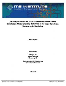
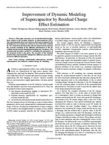
Application to 2D TTI acoustic wave equation We have applied this discretization strategy to equation 5. The first-order partial derivatives in equation 5 are discretized along the axis of the two coordinate systems 共the classic Cartesian one and the 45° rotated one兲 using O共⌬x2兲 staggered-grid stencils 共Virieux, 1986; Saenger et al., 2000兲. The resulting stencils are referred to as Cartesian system 共CS兲 and rotated system 共RS兲. After discretization, the auxiliary wavefields px, pz, qx, and qz are eliminated from the system to end up with a system of two second-order equations in p and q. The geometry of the staggered grids for the CS and RS stencils is illustrated in Figure 1. The TTI equation is inconsistent with the geometry of the CS stencil. Indeed, the p- and q-wavefields need to be defined at the four corners and in the middle of the cell because of the cross-derivatives in H and H0 共Figure 1b兲. Because we used the O共⌬x2兲 stencil, we performed bilinear interpolation to estimate the value of p and q in the middle of the cell from their values at the four corners. In contrast, no interpolation is required for the RS stencil because the p- and q-wavefields and the auxiliary wavefields px, pz, qx, and qz are defined in the same grid 共Figure 1a兲. After discretization and linear combination of the two stencils, the system of second-order wave equations can be written in matrix form as
冉
M p Ⳮ w1Ar Ⳮ 共1 ⳮ w1兲Ac
w1Br Ⳮ 共1 ⳮ w1兲Bc
w1Cr Ⳮ 共1 ⳮ w1兲Cc
M q Ⳮ w1Dr Ⳮ 共1 ⳮ w1兲Dc
⫻
冉冊 冉冊 p
q
⳱
0 0
,
冊 共6兲
where M p denotes the diagonal mass matrix of coefficients 2 / 0. Blocks Ar, Br, Cr, Dr and Ac, Bc, Cc, Dc form the stiffness matrices for the RS and CS stencils, respectively. The coefficient w1 controls the respective weight of the two stencils; it is determined during dispersion analysis by minimizing the phase-velocity dispersion. The mixed-grid stencil contains nine coefficients spanning over two grid intervals 共Figure 2; Appendices A and B兲. This implies that each of the four 共nx ⫻ nz兲2 blocks of the matrix in equation 6 has nine nonzero coefficients per row. The symmetric band-diagonal pattern of each submatrix is the same as that shown by Hustedt et al. 共2004兲 for the isotropic acoustic wave equation 共Hustedt et al., 2004; their Figure 10a兲. In the case of elliptic anisotropy, the q-wavefield is nil; therefore, only the upper-left block remains in equation 8.
Downloaded 17 Nov 2009 to 86.219.18.209. Redistribution subject to SEG license or copyright; see Terms of Use at http://segdl.org/
2D acoustic wave modeling in TTI media The coefficients of submatrices Ar, Br, Cr, and Dr are given in Appendix A; those of submatrices Ac, Bc, Cc, and Dc are given in Appendix B.
agonal term of the mass matrices is replaced by its weight average 共Stekl and Pratt, 1998兲:
冉
2 2 wm2 2 2 2 2 → wm1 Ⳮ Ⳮ Ⳮ Ⳮ 4 iⳭ1,j iⳮ1,j i,jⳭ1 i,jⳮ1 ij ij
Antilumped mass
Ⳮ
One can also introduce a mass term averaging over the nine grid points of the mixed-grid stencil to improve stencil accuracy. The di-
(i,j–1)
(i,j)
(i–1,j+1)
(i,j+1)
(i+1,j)
iⳭ1,jⳮ1
冊
共7兲
,
p P ikh共m cos Ⳮn sin 兲 ⳱ e q Q
共8兲
Here, k ⳱ / cP0 is the wavenumber, h is the grid interval, is the in-
z′
a)
∋
1.000
b) ∼P vph
0.995
0.990
(i+1,j–1)
0.2
0.1
0.0
-0.1
-0.2 -0.2
0.985
x (i,j)
2
To assess the accuracy of the mixed-grid stencil, we perform a classical harmonic dispersion analysis for infinite homogeneous media. This dispersion analysis is applied to the RS, CS, and mixed-grid stencils. We insert the following discrete plane wave in the discrete wave equation for a homogeneous medium:
:p ,p ,q ,q ,b x z x z
(i–1,j)
Ⳮ
冉冊 冉冊
: p, q, δ, , θ
(i,j–1)
iⳮ1,jⳭ1
(i+1,j+1)
z
(i–1,j–1)
2
DISPERSION ANALYSIS
x (i–1,j)
共1 ⳮ wm1 ⳮ wm2兲 2 2 Ⳮ 4 iⳭ1,jⳭ1 iⳮ1,jⳮ1
(i+1,j–1)
Relative error in z-direction (%)
(i–1,j–1)
Ⳮ
冉
冊
where we introduce two new mass coefficients wm1 and wm2, determined jointly with w1 during the dispersion analysis.
x′
a)
T79
-0.1
0.0
0.1
0.2
Relative error in x-direction (%)
0
0.05
0.10
0
0.05
0.10
0.15
0.20
0.25
0.15
0.20
0.25
b)
(i+1,j)
1.000
∼
0.995
S v ph
(i–1,j+1)
(i,j+1)
(i+1,j+1)
0.990
z : p, q, δ, , θ ∋
:p ,p ,q ,q ,b x z x z : p, q
Figure 1. Staggered-grid geometries. 共a兲 RS staggered-grid stencils. 共b兲 CS staggered-grid stencils. The CS stencil requires estimating the p- and q-wavefields in the middle of the cell 共dash squares兲. These are estimated by bilinear interpolation using the values at the four nodes of the cell.
0.985
1/G
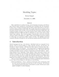
Figure 2. Normalized phase velocity as a function of the number of grid points per wavelength for the 共a兲 P-wave and 共b兲 S-wave modes. The dispersion curves are computed with the mixed-grid stencil for propagation angles of 0°, 15°, 30°, 45°, 60°, and 75° and for Thomsen’s parameters ␦ ⳱ 0.1 and ⑀ ⳱ 0.25. The inset in 共a兲 shows the relative error in percentages of the P-wave phase velocity for G ⳱ 5, P ⳮ 1兲 ⫻ 100 共see text for details兲. The maximum error is i.e., 共˜vphase less than 0.2%.
Downloaded 17 Nov 2009 to 86.219.18.209. Redistribution subject to SEG license or copyright; see Terms of Use at http://segdl.org/
T80
Operto et al.
cidence angle of the plane wave, x ⳱ mh, and z ⳱ nh. This leads to a system of equations in P and Q of the form
冤冢 冣 2 cP2 0
0
0
2 cP2 0
冉 冊冉 2
kG Ⳮ 2
a11 a12 a21 a22
冥
C共w1,wm1,wm2兲 ⳱ 兺 兺 兺 兺 关f共G, ,␦ ,⑀ , 兲兴2, 共11兲
冊冉 冊 冉冊
M
0 P ⳱ , 0 Q
共9兲
where the expression of the coefficients a11, a12, a21, and a22 are given in Appendix C for the RS and CS stencils; G denotes the number of grid points per wavelength, G ⳱ 2 / kh. The two eigenvalues e ⳱ ⳮ 2 / cP2 0 of the matrix M are provided by the roots of the characteristic polynomial det共M ⳮ eI兲 ⳱ 0. We can infer from their expressions the numerical phase velocities of the two modes:
冉 冊 冑冋 冉 冊 冑冋
vPph ⳱ Ⳳ
⫻
vSph ⳱ Ⳳ
⫻
c P0G 2
a11 Ⳮ a22 ⳮ Ⳮ 2
冑
共a11 Ⳮ a22兲2 4
册
ⳮ a11a22 Ⳮ a12a21 ,
c P0G 2
ⳮ
a11 Ⳮ a22 2
ⳮ
冑
共a11 Ⳮ a22兲2 4
册
ⳮ a11a22 Ⳮ a12a21 ,
共10兲 where vPph corresponds to the P-wave mode and vSph corresponds to the S-wave mode. For ⑀ ⬍ ␦ , the term beneath the outer square root is negative for vSph, which implies that the S-wave will grow exponentially during modeling, leading to numerical instabilities. This is consistent with the analytical plane-wave analysis of the VTI acoustic wave equation of Alkhalifah 共2000兲, which shows that one set of complex-conjugate solutions is unstable when ⑀ ⬍ ␦ 共Alkhalifah, 2000; solution a2 in his Figure 1兲. The instability of the S-wave mode is also shown by the expression of the S-wave phase velocity, which becomes imaginary when ⑀ ⬍ ␦ and VS0 ⳱ 0 共Grechka et al., 2004; their equations 1 and 5兲. In spite of the intrinsic instability of the S-wave mode, we see later that we can perform stable numerical simulations of the P-wave mode when ⑀ ⬍ ␦ using our frequency-domain method. In fact, we show that no S-waves are excited during frequency-domain simulation when ⑀ ⬍ ␦ . We suggest that the excitation of the unstable S-wave mode is cancelled out by the absorbing boundary conditions implemented in the frequency-domain boundary value problem. Table 1. Optimal weighting coefficients for the anisotropic mixed-grid stencil. wm1 0.6291844
We apply the same dispersion analysis to the mixed-grid stencil. To estimate the weighting coefficients w1, wm1, and wm3, we define the following cost function:
wm2
w1
0.3708126
0.4258673
G
␦
⑀
with the function f defined as f共G, ,␦ ,⑀ , 兲 ⳱ 1 ⳮ ˜v phP . Here, ˜v phP is the numerical phase velocity normalized by the exact P-wave velocity for VTI media. The exact P- and S-wave velocities for VTI media are given in Tsvankin 共2001; his equation 1.55兲. We minimize the cost function by considering simultaneously four values of G 共0.1, 0.15, 0.2, and 0.25兲, four representative values of the 共 ␦ ,⑀ 兲 pairs taken from Thomsen 共1986兲 关共0.148 0.091兲, 共ⳮ0.012 0.137兲, 共0.057 0.081兲, and 共0.1 0.225兲兴, ⳱ 0, and six values of ranging from 0° to 75°. The cost function is minimized with a very fast simulated annealing algorithm 共Sen and Stoffa, 1995兲. We obtain the coefficients wm1 ⳱ 0.6291844, wm2 ⳱ 0.3708126, and w1 ⳱ 0.4258673 for a final rms of 1.4947164E-04 共Table 1兲. The normalized phase-velocity dispersion curves for the two modes are shown in Figure 2 for ranging from 0° to 75° and for ␦ ⳱ 0.1 and ⑀ ⳱ 0.2. These curves can be compared with those obtained with the RS and CS stencils, respectively, to determine the accuracy improvement provided by the mixed-grid and antilumped mass strategies 共see Operto et al., 2007a; their Figure 2a and b兲. The dispersion curves for the P-mode shown in Figure 2a suggest that four grid points per wavelengths will provide sufficiently accurate simulations of P-waves in homogeneous media. Indeed, the maximum phase-velocity error is 0.4% for G ⳱ 4, whereas the average error is on the order of 0.1% the value of I 共Figure 2a兲. The phase-velocity dispersion curves of the second mode normalized by the exact phase velocity of the SV-wave confirm that the second mode of the TTI acoustic equation corresponds to an S-wave. This curve is not shown for ⳱ 0 because the phase velocity of the S-wave is nil on the symmetry axis, through construction of the acoustic equation of Alkhalifah 共2000兲. We verified during dispersion analysis that this velocity remains nil after discretization.
SOURCE EXCITATION It is well acknowledged that applying a pressure source in the acoustic VTI/TTI equation leads to exciting an S-wave with a characteristic diamond shape 共Alkhalifah, 2000; Grechka et al., 2004; Zhang et al., 2005兲. Anderson et al. 共2008兲 propose to modify the pressure source to cancel the shear strains and therefore the excitation of the S-waves in acoustic anisotropic media. The moment tensor source equivalent to a pressure source can be written as
dM 11 ⳱ ⳮs1 P, dt dM 33 ⳱ ⳮs3 P. dt
共12兲
For an isotropic source, the weighting coefficients s1 and s3 equal one. In anisotropic acoustic media, we use s1 ⳱ 2共共C11 Ⳮ C13兲 / 共C11 ⳭC13 Ⳮ C13 Ⳮ C33兲兲 and s3 ⳱ 2共共C13 Ⳮ C33兲 / 共C11 Ⳮ C13 ⳭC13 ⳭC33兲兲, where the Cij coefficients denote the elastic moduli.
Downloaded 17 Nov 2009 to 86.219.18.209. Redistribution subject to SEG license or copyright; see Terms of Use at http://segdl.org/
2D acoustic wave modeling in TTI media We first apply the isotropic and anisotropic moment tensor sources to the 2D VTI elastodynamic system for which the S-wave velocity on the symmetry axis is set to zero 共this gives C44 ⳱ 0兲 to mimic acoustic propagation 共Anderson et al., 2008兲:
冦
xx vx ⳱b x t vz zz ⳱b t z xx vx vz ⳱ C11 Ⳮ C13 t x z zz vx vz ⳱ C13 Ⳮ C33 t x z
冧
.
共13兲
Note that equation 13 is not equivalent to the acoustic equation considered in our study. The anisotropic moment tensor source can be implemented in equation 13 by incrementing at each time step the normal stresses xx and zz by ⳮs1 P and ⳮs3 P, respectively 共Coutant et al., 1995兲. We discretize equation 13 in the time domain using the RS stencil 共Saenger et al., 2000兲. The source wavelet is a Ricker wavelet with a 4-Hz dominant frequency. The P-wave velocity on the symmetry axis is 2 km/ s, ␦ ⳱ 0.1, and ⑀ ⳱ 0.2. The grid interval is 10 m. The RS stencil requires that the spatial distribution of the point source with a 2D Gaussian function is spread to guarantee an effective coupling between the stress and the particle velocity staggered grids 共Hustedt et al., 2004兲. Here, we use horizontal and vertical correlation lengths of 40 m. Snapshots for the isotropic 共s1 ⳱ s3 ⳱ 1兲 and anisotropic 共s1 ⳱ 2共共C11 Ⳮ C13兲 / 共C11 Ⳮ C13 Ⳮ C13 Ⳮ C33兲兲 and s3 ⳱ 2共共C13 Ⳮ C33兲 / 共C11 Ⳮ C13 Ⳮ C13 Ⳮ C33兲兲 moment tensor sources are shown in Figure 3a and b. Use of the anisotropic source helps to attenuate the S-wave efficiently. However, the spatial smoothing of the point source is a second feature required to attenuate the S-wave. Indeed, the S-wave has a higher wavenumber content than the P-wave 共see Bale, 2007; his Figure 1a兲. Therefore, a spatial smoothing of the source can be found such that it partially low-pass filters the S-wave without affecting the P-wavefront. We also performed a simulation with the CS stencil that does not require smoothing the source 共Hustedt et al., 2004兲. Without smoothing the point source, the attenuation of the S-wave was much less efficient than in Figure 3b. This is not a result of the stencil geometry because we verified that the CS and the RS stencils led to the same S-wave attenuation when the source was smoothed in the same manner. In a second step, we applied the isotropic and anisotropic moment tensor sources to the acoustic VTI equation, recast as a first-order hyperbolic system 共equation 3兲 in the time domain 共Figure 3c and d兲. The RS stencil was used to discretize equation 3. The pressure source was implemented with horizontal and vertical dipoles applied to the third and fourth equations of expression 3. Each dipole was weighted by coefficients s1 and s2. The source was smoothed with a 2D Gaussian function; horizontal and vertical correlation lengths were 40 m. Although the S-wave was weakened, it was not fully canceled when the anisotropic moment tensor source was used 共Figure 3d兲. To remove the S-wave efficiently, a correlation length as
T81
great as 80 m must be used, which leads to significant attenuation and distortion of the P-wavefront 共Figure 3e and f兲. So far, we have failed to remove the S-wave excitation efficiently at the source in the case of the acoustic anisotropic equation when the source is located in a medium with ␦ ⬍ ⑀ . To avoid exciting the S-wave, the source can be set in an isotropic layer or in an elliptically anisotropic layer.
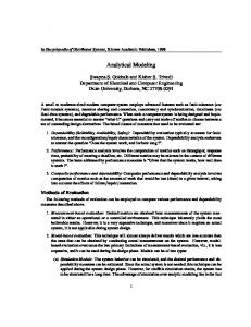
PML ABSORBING BOUNDARY CONDITION PML absorbing boundary conditions provided a good absorption of the waves on the edges of the model. However, we have observed instabilities in the PML layers in the TTI case 共i.e., when the symmetry axis is tilted with respect to the vertical and horizontal PML-PML interfaces兲. These instabilities, which are seen only when the number of grid points per wavelength is significantly greater than four and when ⑀ ⬎ ␦ , are likely caused by the S-waves. When the grid interval is set according to the rule of four grid points per P-wavelength, the S-waves are affected strongly by numerical dispersion, which may cancel out the instability 共Hu, 2001兲. When ⑀ ⬍ ␦ , no Swaves are excited during frequency-domain modeling and no instability is seen, whatever the discretization. The instability of PMLs in anisotropic media is studied theoretically by Bécache et al. 共2003兲. They show in their Figure 13 that a necessary condition to guarantee the stability of PMLs is that, along the velocity curves, the slowness vector and the group velocity are oriented in the same way with respect to the Cartesian axis 共i.e., the PML-PML interfaces兲. We plot the velocity curves for the S-waves in a homogeneous medium for a vertical symmetry axis and for a 45° rotated axes 共Figure 4兲. When the symmetry axis is tilted, the group velocity vector and the slowness vector do not satisfy the geometric stability criterion of Bécache et al. 共2003兲 共Figure 4b兲, contrary to the case where the symmetry axis is vertical 共Figure 4a兲. Further study is required to remove this instability.
NUMERICAL EXAMPLES In this section, we validate our method against analytical solutions along the symmetry axis and numerical solutions computed in 2D VTI elastic media with a classic staggered-grid velocity-stress FDTD method.
Simulation in homogeneous media We first validate the method against an analytical solution along the symmetry axis available for class IV TI media 共Payton, 1983兲.
Strong anisotropy: Zinc crystal For the simulation, we consider a zinc crystal 共Carcione et al., 1988; Komatitsch et al., 2000兲; properties are summarized in Table 2. The model measures 3300⫻ 3300 m with grid intervals for the acoustic FDFD and elastic FDTD simulations of 15 and 5 m, respectively. The source is in the middle of the grid. The source wavelet is a Ricker wavelt with a dominant frequency of 17 Hz. A horizontal receiver line is located above the source at a distance of 1 km. The symmetry axis is vertical.
Downloaded 17 Nov 2009 to 86.219.18.209. Redistribution subject to SEG license or copyright; see Terms of Use at http://segdl.org/
T82
Operto et al.
Snapshots computed with the acoustic FDFD and elastic FDTD methods are shown in Figure 5. The analytical velocity and wavefront contours for the quasilongitudinal and quasitransverse modes are superimposed in both snapshots 共Carcione et al., 1988兲. Good kinematic agreement is obtained between the analytical P- and S-velocity curves and the VTI elastic wavefronts 共Figure 5b兲, whereas some mismatch is seen between the qP-wave analytical velocity curve and the VTI acoustic wavefront for directions of propagation midway between the symmetry axis and its perpendicular. Comparisons between the two snapshots of Figure 5 also suggest strongly overestimated amplitudes in the acoustic solution perpendicular to the symmetry axis.
a) –4
–4
–3
–2
Distance (km) 1 0 –1
b) 2
3
4
–4
–4
–3
–2
–2
–1
–1
0
0
1
1
2
2
3
3
Depth (km)
–3
Depth (km)
-4
–4
–3
–2
–1
0
1
2
3
4
d) –4
-3
–3
-2
–2
-1
–1
0
0
1
1
2
2
3
3
4
e) –4
2
3
4
0
1
2
3
4
0
1
2
3
4
–2
–1
–3
–2
–1
–3
–2
–1
Figure 3. Source implementation. 共a兲 Simulation using the RS staggered-grid stencil and an isotropic pressure source. The wave equation is the elastodynamic system within which the S-wave velocity on the symmetry axis is set to zero 共equation 13兲. 共b兲 As for 共a兲, except an anisotropic pressure source is used 共see text for details兲. 共c兲 As for 共a兲, except the acoustic anisotropic equation considered in this study is used for the simulation; an isotropic pressure source is used. 共d兲 As for 共c兲, except an anisotropic pressure source is used; note the less efficient attenuation of the S-wave than in 共b兲. 共e–f兲 As for 共c兲, except the horizontal and vertical correlation lengths of the Gaussian function used to smooth the point source are 共e兲 20 and 共g兲 80 m.
4 –4
–3
–2
–1
0
1
2
3
4
f) -4
–4
–3
-3
–2
-2
–1
-1
0
0
1
1
2
2
3
3
4
4
Depth (km)
Distance (km) 1 0
–3
4
4
c)
Time-domain synthetic seismograms computed with the acoustic FDFD and elastic FDTD methods are compared in Figures 6 and 7. Good kinematic and dynamic agreement between the two solutions is obtained only for propagation directions close to the symmetry axis. This is further confirmed by a comparison of analytical seismograms and VTI acoustic seismograms recorded along the symmetry axis, which shows good agreement 共Figure 7兲. For the zinc crystal, ⑀ ⳱ 0.83 is significantly smaller than ␦ ⳱ 2.7 共Table 2兲. This set of Thomsen’s parameters should lead to unstablesimulation of the S-waves with the VTI acoustic equation. In contrast, we did not see any excitation of S-waves in our frequencydomain simulation when ⑀ ⬍ ␦ 共Figure 5兲, and simulation of the
Downloaded 17 Nov 2009 to 86.219.18.209. Redistribution subject to SEG license or copyright; see Terms of Use at http://segdl.org/
2D acoustic wave modeling in TTI media
a) –1.5
–1.0
Distance (km) –0.5 0.0 0.5
1.0
1.5
–1.5
–1.0
–0.5
1.0
1.5
–1.5 –1.0
Depth (km)
P-waves remained stable. A possible reason is that the absorbing conditions implemented in the boundary-value frequency-domain problem cancel out this unstable mode. The ability to perform stable frequency-domain simulation of P-waves without exciting undesired S-waves when ⑀ ⬍ ␦ is confirmed in the following section. This numerical example confirms that the acoustic approximation of wave propagation in VTI media does not lead to accurate solutions in cases of strong anisotropy. However, a comparison between numerical and analytical solutions along the symmetry axis provides the first validation of the implementation of the VTI acoustic mixedgrid stencil.
T83
–0.5 0.0 0.5
Weak anisotropy: Sediment
Simulation in anticline medium
1.0 1.5
b)
0.0
0.5
–1.5 –1.0
Depth (km)
We repeat the numerical experiment on a material involving weaker anisotropy with the medium properties summarized in Table 2, for this example, ⑀ ⬎ ␦ . The grid dimensions, the source wavelet, and the acquisition system are the same as in the previous case. The symmetry axis is vertical. Snapshots computed with the acoustic FDFD and the elastic FDTD methods are compared in Figure 8a. The diamond-shaped S-wave is seen in the acoustic snapshot because ⑀ ⬎ ␦ . Good kinematic agreement is now seen between the acoustic snapshot and the P-wavefront curve, whatever the direction of propagation. Acoustic FDFD and elastic FDTD seismograms show good agreement from kinematic and dynamic viewpoints 共Figure 8b兲. This numerical example shows that the acoustic approximation of VTI wave propagation provides accurate simulation in homogeneous media in weak to moderate anisotropy. We next consider the same simulation but for a 45° tilted symmetry axis. A snapshot computed with the acoustic FDFD method is shown in Figure 9a. The receiver line is rotated by 45° to compare the TTI acoustic seismograms with the VTI elastic ones computed with the FDTD method. Good agreement is obtained between TTI acoustic seismograms and VTI elastic seismograms 共Figure 9b兲. The PMLs cause strong instabilities because the grid interval cannot be matched to each frequency when computing time-domain seismograms from a frequency-domain algorithm 共Figure 9a兲. For this simulation, the PML instability is mitigated by the C-PML functions and complex-valued frequencies, used to remove wraparound 共Mallick and Frazer, 1987兲.
–0.5 0.0 0.5 1.0 1.5
Figure 4. Geometric interpretation of the PML instability. Phase 共red兲 and group 共blue兲 velocity curves of the S-wave for the 共a兲 VTI and 共b兲 TTI cases. In 共b兲, the tilt angle is 45°. The dashed arrows are along the velocity group vector; the solid arrows are along the slowness vectors, which are perpendicular to the wavefront. For the VTI case, both vectors have the same orientation with respect to the Cartesian axis 共PML-PML interfaces兲; for the TTI case, they point in opposite directions.
We now consider a heterogeneous medium composed of two layers delineated by a bell-shaped interface 共Figure 10a兲. The properties of the two media are summarized in Table 3. The upper layer is homogeneous, whereas the P-wave velocity increases linearly with depth in the bottom layer to Table 2. Properties of the zinc and sedimentary media for validation in generate turning waves of significant amplitudes homogeneous media. at long offset. The velocity gradient for the ⳮ1 P-wave velocity in the bottom layer is 0.2 s . The other parameters are constant in the bottom ␦ ⑀ VS VP layer. 共m/s兲 共m/s兲 共kg/ m3兲 Medium This example is designed to test the accuracy Zinc 2955.06 2361 7100 2.70968 0.830645 of the numerical scheme when the dip of the structures varies with respect to the symmetry Sediments 4000 2309 2500 0.02 0.1 axis, which is vertical in this simulation. We set
Downloaded 17 Nov 2009 to 86.219.18.209. Redistribution subject to SEG license or copyright; see Terms of Use at http://segdl.org/
共°兲 0 0
T84
Operto et al.
⑀ ⬍ ␦ in the upper medium, where the source is located, to avoid exciting the undesired S-waves at the source. The S-wave velocity used for the VTI elastic simulation is constant in the whole model and is equal to 2.361 km/ s. The explosive source is a Ricker wavelt with a dominant frequency of 17 Hz. The model dimensions are 16,000 ⫻ 5000 m, and the grid intervals are 10 and 4 m for the VTI acousticFDFD and elastic FDTD simulations, respectively. The source is at a distance of 3.5 km and a depth of 0.4 km. A line of 171 receivers positioned every 40 m is 100 m above the source. An 11.7-Hz monochromatic wavefield computed with the acoustic FDFD method shows a spurious arrival transmitted below the anticline 共i.e., where the dip of the bell-shaped interface is not along or
Distance (km)
Depth (km)
a)
Depth (km)
b)
perpendicular to the symmetry axis兲 and superimposed on the transmitted P-wavefield 共Figure 10b兲. This event is not seen at the vertex of the source where the interface is perpendicular to the symmetry axis. The spurious event corresponds to the conversion from the P-mode to the S-mode in the lower medium. The amplitudes of these P-to-S converted waves increase with the contrast between ␦ and ⑀ at the interface. We repeat the simulation after smoothing the ␦ and ⑀ models with a 2D Gaussian filter of horizontal and vertical correlation lengths of 60 m 共Figure 10c兲. In this case, the P-to-S converted waves are removed 共compare Figure 10b and c兲. We also verify that no P-to-S conversion occurs when ⑀ is lower than ␦ in the two layers of the model. The VTI acoustic and elastic seismograms computed in the model of Figure 10a are compared in Figure 11. The acoustic seismograms are computed in the models without smoothing the ␦ and ⑀ models. Reasonable agreement is obtained between the two sets of seismograms, although there is some mismatch between the amplitude-versus-offset behavior of the first arrival 共illustrated by the variation of the polarity of the residual seismograms with offset in Figure 11c兲. To reveal the arrivals generated by the P-to-S conversion at interfaces more clearly, we performed a simulation in a model composed of two homogeneous half-spaces separated by a dipping interface 共Figure 12兲. The dip of the interface is 30°, whereas the symmetry axis is vertical. The properties of the two half-spaces are given in Table 3. A 17-Hz monochromatic wavefields for the p- and q-wavefield 共Figure 12a and b兲 as well as a time-domain snapshot 共Figure 12c兲 show that the dominant spurious event is an interface wave, labeled I in Figure 12c, that propagates along the interface with the P-wave velocity of the upper medium in the direction of the interface. This is first shown by the continuity between the direct P-wavefront in the upper medium and the head wavefront at the interface 共Figure 12c兲. The event is further confirmed by the seismograms of Figure 12d, recorded by a line of receivers 500 m below the interface. The slope of arrival I corresponds to the P-wave velocity in the upper medium for an incidence angle along the interface. We also observe the head wave labeled I⬘, which also propagates along the interface with the P-wave velocity of the lower medium in the direction of the interface. The transmitted S-wavefront is rather difficult to interpret in Figure 12c. Interestingly, we performed one other simulation, where the interface was horizontal and the symmetry axis was vertical 共Figure 13兲. In this case, the q-wavefield shows an evanescent wavefront propagating along the interface, and no interface waves propagate in the lower layer.
Simulation in the 2D anisotropic overthrust model
Figure 5. Modeling for the zinc model — VTI 共a兲 elastic and 共b兲 acoustic snapshots. The blue and red curves are the group and phasevelocity curves, respectively. The white line is the receiver line. The source is in the middle of the medium.
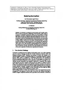
We now consider the simulation in a 2D section of the anisotropic overthrust model 共Figure 14兲. The symmetry axis is vertical. The model dimensions are 20⫻ 4.4 km. The Thomsen’s parameters ␦ and ⑀ range between ⳮ0.176602 and 0.06 and between 0 and 0.2, respectively. The model embeds isotropic, elliptic anisotropic, and VTI layers. For the VTI elastic simulation, we consider a homogeneous S-wave velocity of 1.3 km/ s to minimize the footprint of the S-waves. The explosive source is a Ricker wavelet of 6-Hz dominant frequency. The source is at a distance of 4 km and depth of 0.4 km with a line of 501 receivers spaced at 40-m intervals at 100 m depth. The grid interval for the acoustic simulation is 20 m, providing a fi-
Downloaded 17 Nov 2009 to 86.219.18.209. Redistribution subject to SEG license or copyright; see Terms of Use at http://segdl.org/
2D acoustic wave modeling in TTI media nite-difference grid measuring 301⫻ 1081, including 800-m-thick PMLs along the four edges of the model. The grid interval for the elastic simulation is 10 m. Acoustic and elastic snapshots can be compared in Figure 15. The footprint of the converted S-waves described in the previous section is seen clearly in the VTI layers of the acoustic snapshots. These events did not affect the acoustic seismograms recorded in the vicinity of the surface where the medium is isotropic because these S-waves remain confined to the VTI layers. The acoustic and the elastic seismograms compare well in Figure 16. We now compare the computational efficiency of the FDFD and the FDTD approaches to compute monochromatic wavefields for
Figure 6. Modeling for the zinc model. 共a兲 Acoustic seismograms. 共b兲 Elastic seismograms. 共c兲 Direct comparison between the acoustic 共dashed gray兲 and elastic 共solid black line兲 seismograms.
a)
T85
multiple sources. These monochromatic wavefields typically represent the amount of data processed during one inversion iteration of single-frequency, frequency-domain FWI 共Sirgue and Pratt, 2004; Brenders and Pratt, 2007a兲. In FDTD modeling, monochromatic wavefields can be computed by discrete Fourier transform in the loop over time steps 共Sirgue et al., 2008兲. The FDFD simulation in the overthrust model was performed using two nodes of a PC cluster, each node comprising two dual-core 2.4-GHz processors, providing 19.2 Gflops of peak performance per node. Each node had 8 Gb of RAM. The interconnection network between processors was Infiniband 4X. We used the massively parallel MUMPS direct solver to perform LU factorization and the for-
b)
c)
Downloaded 17 Nov 2009 to 86.219.18.209. Redistribution subject to SEG license or copyright; see Terms of Use at http://segdl.org/
Operto et al.
a)
Distance (km) –0.5 0.0 0.5
1.0
1.5
–0.5 0.0
0.5
1.0
1.5
–1.5 –1.0 –0.5 0.0 0.5 Offset (km)
1.0
1.5
–1.5 –1.0 –1.5 –1.0 Depth (km)
ward/backward substitutions in the FDFD modeling 共Amestoy et al., 2006; Sourbier et al., 2009a, 2009b兲. The elapsed time for one parallel factorization was 68 s. The elapsed time to compute solutions for 64 sources by forward/backward substitutions was 8 s, leading to an elapsed time of 0.125 s per source. For elliptic anisotropy, the elapsed times for the factorization and for the 64 forward/backward substitutions decreased considerably to 3.5 s and 2 s, respectively, because the number of unknowns in the system decreased by a factor of two 共the q-wavefield is nil兲. The sequential elastic FDTD simulations took 1606 and 173 s for grid intervals of 10 and 20 m, respectively. The duration of the seismograms was 6 s. A grid interval of 10 m corresponds to the discretization required by an elastic FDTD simulation involving minimum S-wave velocities of 1 km/ s and a maximum frequency of 20 Hz for an O共⌬x4兲 accurate stencil. A grid interval of 20 m was used for the FDFD simulation, corresponding to the discretization required by an acoustic simulation for a maximum frequency of 20 Hz. Considering a coarse-grained parallelism over shots for FDTD simulation 共which has an efficiency of one兲, the elapsed times to perform the modeling for the 64 shots distributed over the 8 MPI processes would be 1606⫻ 64/ 8 ⳱ 12,848 s and 173⫻ 64/ 8 ⳱ 1384 s for the 10- and 20-m grid intervals, respectively. The elapsed time of the acoustic and elastic FDTD simulations are significantly greater than the elapsed time of the acoustic FDFD simulation, i.e., 68Ⳮ 8 ⳱ 76 s. These differences would increase dramatically with the number of sources. Thus, this numerical experiment confirms the conclusions inferred from the theoretical complexities of 2D FDFD and FDTD modeling 共see Nihei and Li 共2007兲 for a review兲 concerning the superiority of the frequency domain to compute monochromatic wavefields for many sources.
–0.5 0.0 0.5 1.0 1.5
b)
–1.5 –1.0 –1.5 –1.0
Depth (km)
T86
–0.5 0.0 0.5 1.0
DISCUSSION Two features of the modeling method presented in this study are the frequency-domain formulation and the acoustic approximation
1.5
c)
0.8
Offset = 700 m
Time (s)
0.6
0.4 0.2
Offset = 1600 m 0.0
0.1
0.2
0.3
0.4
0.5
Time (s)
0.6
0.7
0.8
0.9
Figure 7. Modeling for the zinc model, comparing the analytical 共solid line兲 and numerical acoustic seismograms on the symmetry axis for two offsets 共700 and 1600 m兲. The difference is plotted with the dashed lines.
Figure 8. Modeling for the homogeneous sediment model — VTI 共a兲 acoustic and 共b兲 elastic snapshots. Time is 0.3 s. Velocity 共blue兲 and wavefront 共red兲 curves for the P- and S-modes are superimposed. 共c兲 Direct comparison between acoustic 共dashed gray line兲 and elastic 共solid black line兲 seismograms. Difference is plotted with dashed black seismograms. The strong residual at 0 km offset and 0.6– 0.8 s traveltimes is the result of the S-wave in the acoustic solution.
Downloaded 17 Nov 2009 to 86.219.18.209. Redistribution subject to SEG license or copyright; see Terms of Use at http://segdl.org/
2D acoustic wave modeling in TTI media to model seismic wavefields in anisotropic media. Our main motivation behind the frequency domain and the acoustic approximation is to design a computationally efficient forward problem for imaging TTI media by frequency-domain FWI. Our numerical stencil provides sufficiently accurate solutions of the acoustic TTI wave equation when four grid points per wavelength are used for discretization. This discretization is suitable for FWI where the resolution limit is a half-wavelength. Although the viscoacoustic TTI wave equation requires modeling two wavefields 共the pressure wavefield plus the auxiliary wavefield q兲 as the elastic wave equation 共two particle velocity wavefields兲, acoustic modeling remains significantly less demanding computationally than elastic modeling, mainly because the elastic wave
a)
T87
equation is discretized according to the minimum S-wavelength. We also verify numerically the superior computational efficiency of the frequency-domain approach compared to time-domain approaches for multisource modeling of monochromatic wavefields. Our second motivation behind the acoustic approximation is to mitigate the ill-posedness of FWI. Part of FWI ill-posedness results from partial coupling between different classes of parameters.Apossible way to mitigate the ill-posedness is to consider simplifying assumptions in the physics of wave propagation — in other words, to limit the number of parameter classes in the medium parameterization. It is also worth noting that the footprint of anisotropy in P-waves is less complex than that affecting S-waves because P-waves are not split in two modes yet have a hyperbolic reflection moveout in anisotropic media 共Tsvankin, 2001兲. The ill-posedness of the FWI also results from the sensitivity of local optimization approaches for inaccuracies of the starting model. This sensitivity increases in elastic FWI because S-waves have higher resolution power than P-waves as a result of their smaller wavelengths. The higher resolution power of S-waves requires more accurate S-wave-velocity starting models or a lower starting frequency to make the inversion converge toward acceptable velocity models 共Brossier et al., 2008兲.
a)
b)
PML instability
b)
Time (s)
0.6 0.5
c)
0.4 0.3 0.2 –1.5
–1.0
–0.5
0.0 0.5 Offset (km)
1.0
1.5
Figure 9. 共a兲 Snapshot computed for the TTI acoustic homogeneous medium. The symmetry axis is rotated by 45° with respect to the vertical. The white line denotes the position of the receivers. The arrow points out spurious signals resulting from PML instability. 共b兲 Direct comparison between the TTI acoustic 共dashed gray line兲 and VTI elastic 共solid black line兲 seismograms.
Figure 10. 共a兲 Anticline model. 共b兲 Monochromatic wavefield. Note the spurious event transmitted in the lower medium, where the dip of the interface is significant with respect to the symmetry axis. 共c兲 As for 共b兲, except the ␦ and ⑀ models are smoothed with a 2D Gaussian filter of horizontal and vertical correlation lengths equal to six times the grid interval. Smoothing the contrast between the Thomsen parameters removes the artifact.
Downloaded 17 Nov 2009 to 86.219.18.209. Redistribution subject to SEG license or copyright; see Terms of Use at http://segdl.org/
T88
Operto et al.
Indeed, the reliability of the acoustic anisotropic approximation in the framework of FWI can be questioned because acoustic media are intrinsically isotropic. The numerical experiments we present suggest that the viscoacoustic TTI wave equation is sufficiently accurate from a dynamic viewpoint for weak to moderate anisotropic media.
Regarding the footprint of the S-waves in viscoacoustic TTI modeling, the excitation of S-waves can be cancelled at the source by setting the source in an isotropic layer or in an elliptically anisotropic layer. Excitation of S-waves at the source can be cancelled out pragmatically by setting a small, smoothly tapered circular region with
Table 3. Properties of the anticline model. The P-wave velocity increases linearly with depth in the bottom layer with a gradient of 0.2 sⴑ1. The velocity on top of the layer is provided. The other parameters are constant. Layer Top Bottom
a)
VP 共m/s兲 2955.06 4820.73 共on top兲
VS 共m/s兲
共kg/ m3兲
␦
⑀
共°兲
2361.66 2361.66
2200 2500
0.143 0.06
ⳮ0.035 0.11
0 0
Figure 11. Anticline model simulation — 共a兲 acoustic and 共b兲 elastic seismograms. The seismograms are plotted with a reduction velocity of 5 km/ s. Some artificial reflections are seen on the right end of the model in the case of the elastic simulation. 共c兲 Direct comparison between acoustic 共dashed gray line兲 and elastic 共solid black line兲 seismograms. The differences are the thin dashed black line.
b)
c)
Downloaded 17 Nov 2009 to 86.219.18.209. Redistribution subject to SEG license or copyright; see Terms of Use at http://segdl.org/
2D acoustic wave modeling in TTI media
␦ ⳱ ⑀ around the source 共Duveneck et al., 2008兲. The P-to-S-modeconversion at sharp interfaces cannot be removed efficiently without slightly smoothing the ␦ and ⑀ contrasts, which is a last resort in FWI. However, our numerical experiments suggest that the P-to-Smode converted waves do not affect reverse-time-migrated images significantly, possibly because of their small amplitudes 共Duveneck et al., 2008兲. A last issue concerns the extension to 3D modeling. The time and memory complexities of the direct solvers as well as their limited intrinsic scalability prevent large-scale modeling in 3D viscoacoustic TTI media with the approaches we develop 共Operto et al., 2007b兲.
a)
c)
b)
d)
a)
T89
Only elliptic anisotropy can be implemented in 3D FDFD approaches based on a direct solver because it does not introduce computational overhead compared to the isotropic case. For 3D large-scale applications, the acoustic VTI and TTI wave equations can be implemented easily in the time domain with explicit integration schemes 共Duveneck et al., 2008; Fletcher et al., 2008; Lesage et al., 2008兲. The alternative FDFD approaches developed so far for the acoustic isotropic wave equation are based on hybrid direct/iterative solvers 共Sourbier et al., 2008兲 or iterative solvers 共Erlangga and Herrmann, 2008兲. These approaches also can be viewed for 3D viscoacoustic
Figure 12. Monochromatic 共a兲 p- and 共b兲 q-wavefields in the dipping-layer model. 共c兲 Time-domain snapshot. Nomenclature: D — direct P-wave; R — reflected P-wave; T — transmitted P-wave; H — P head wave; I and I⬘ — head waves ensuring the continuity between the transmitted P- and S-wavefronts I⬘ and between the reflected and transmitted S-wavefronts I; E — evanescent interface wave. 共d兲 Time-domain seismograms recorded by a receiver line 500 m below the interface.
Figure 13. Monochromatic 共a兲 p- and 共b兲 q-wavefields in the case of two VTI half-spaces delineated by a flat interface. In this case, the interface wave is evanescent and does not lead to a conic wave in the lower medium.
b)
Downloaded 17 Nov 2009 to 86.219.18.209. Redistribution subject to SEG license or copyright; see Terms of Use at http://segdl.org/
T90
km/s
Distance (km)
Time - offset/6 (s)
Depth (km)
b) ρ
b)
Depth (km)
Time - offset/6 (s)
c) δ
–2
0
2
4
–2
0
2
4
–2
0
2
Offset (km) 6 8
10
12
14
16
10
12
14
16
1 2 3 4 0
6
8
1 2 3 4
d)
c) 4
Depth (km)
ε
a) 0
Depth (km)
a)
Operto et al.
Figure 14. VTI overthrust model. 共a兲 P-wave velocity; 共b兲 density; 共c兲 ␦ ; 共d兲 ⑀ .
a)
Time - offset/6 (s)
3
2
1
0 –4
4 6 8 10 Horizontal offset (km)
12
14
16
Figure 16. Synthetic seismograms computed in the overthrust model: 共a兲 VTI acoustic seismograms; 共b兲 VTI elastic seismograms; 共c兲 direct comparison between acoustic 共dashed gray line兲 and elastic 共solid black line兲 seismograms. The seismograms are plotted with a reduction velocity of 6 km/ s. The source is in an isotropic layer.
b)
CONCLUSION
Figure 15. Simulation in the overthrust model. Acoustic 共top panel兲 and elastic 共bottom panel兲 snapshots for two propagation times: 共a兲 1 and 共b兲 3.8 s. The S-waves affect the acoustic wavefields in the VTI layers of the overthrust model. TTI modeling in the future. Although the approaches we present in this study do not extend to 3D cases easily, efficient 2D algorithms remain useful in assessing the potential and limits of unconventional seismic imaging methods.
We have developed a computationally efficient FDFD method for multisource seismic wave modeling in 2D viscoacoustic TTI media. Comparisons between acoustic and elastic modeling in weak to moderate anisotropic media suggest that the method is sufficiently accurate for FWI from kinematic and dynamic viewpoints. The main limitation of the method is the propagation of S-waves in acoustic VTI and TTI media. Whereas S-wave excitation can be cancelled out pragmatically at the source, the P-to-S mode conversions occur at sharp contrasts between anisotropic parameters. The real footprint of these P-to-S converted waves must be assessed during the summation of the redundant information underlying full-waveform inversion. A last resort to avoid these mode conversions is to smooth the contrast between the anisotropic parameters ␦ and ⑀ slightly. The S-wave mode is unstable in the acoustic anisotropic wave equation when ⑀ ⬍ ␦ , but we observe that the S-waves are not excited during frequency-domain modeling in such media. Therefore, we performed stable simulations of the P-waves in the frequency domain unlike in the time domain. Future studies will involve interfacing the viscoacoustic TTI modeling method into a frequency-do-
Downloaded 17 Nov 2009 to 86.219.18.209. Redistribution subject to SEG license or copyright; see Terms of Use at http://segdl.org/
2D acoustic wave modeling in TTI media
T91
main viscoacoustic full-waveform inversion code to assess the reliability of full-waveform inversion for imaging anisotropic parameters quantitatively.
Gathering the terms with respect to the indices of the p-wavefield gives nine coefficients of the RS stencil for the submatrix Ar of equation 6:
ACKNOWLEDGMENTS
1 biⳭ1/2,jⳮ1/2 biⳮ1/2,jⳭ1/2 Arij ⳱ ⳮ Ⳮ 2 Axij 4 xih xiⳭ1/2 xiⳮ1/2
冉
Access to the high-performance computing facilities of the Mesocentre SIGAMM computer center provided the required computer resources, and we gratefully acknowledge this facility and the support of its staff. This work was conducted within the framework of the SEISCOPE consortium, sponsored by BP, CGGVeritas, ExxonMobil, Shell, and TOTAL. This work was funded partly by the ANR project 共ANR-05-NT05-2-42427兲. We thank Assistant Editor V. Grechka, Associate Editor M. van der Baan, E. Saenger, and two anonymous reviewers for their useful comments. We are especially grateful to V. Grechka for his useful comments on stability constraints in acoustic anisotropic media. We would like to thank W. A. Mulder 共Shell International E&P BV兲 for providing us the anisotropic overthrust model 共http://aniso.citg.tudelft.nl兲.
biⳭ1/2,jⳭ1/2 biⳮ1/2,jⳮ1/2 Ⳮ xiⳭ1/2 xiⳮ1/2
Ⳮ
1 biⳭ1/2,jⳮ1/2 biⳮ1/2,jⳭ1/2 Bx Ⳮ 4 xih2 ij z jⳮ1/2 z jⳭ1/2
ⳮ
biⳭ1/2,jⳭ1/2 biⳮ1/2,jⳮ1/2 ⳮ z jⳭ1/2 z jⳮ1/2
Ⳮ
In this appendix, we provide the expression of the parsimonious RS staggered-grid stencil. The partial derivatives with respect to x and z can be replaced by a linear combination of the partial derivatives with respect to the rotated coordinates x⬘ and z⬘ in equation 5 共Figure 2兲:
冉 冑 冉
冊
1 ⳱ Ⳮ , 冑 x 2 x⬘ z⬘
冊
冋 册 冋 册 g x⬘ g z⬘
⳱ ij
⳱ ij
1
冑2h 关giⳭ1/2,jⳭ1/2 ⳮ giⳮ1/2,jⳮ1/2兴.
We first discretize the first two equations of system 5 using discrete scheme A-2. Then, we define the expression of wavefields px, qx, pz, and qz at the grid positions required by the discrete form of the first two equations of system 5 using discrete scheme A-2. Finally, we inject the resulting expressions of px, qx, pz, and qz into the first two equations to derive the second-order discrete equation in p and q.
冊
biⳭ1/2,jⳭ1/2 biⳮ1/2,jⳮ1/2 Ⳮ , z jⳭ1/2 z jⳮ1/2
Ⳮ
冉 冉 冉 冉
冊
共A-3兲
1 biⳭ1/2,jⳮ1/2 biⳭ1/2,jⳭ1/2 Ax Ⳮ 4 xih2 ij xiⳭ1/2 xiⳭ1/2 1 4 xih 1 4 z jh
冊 冊
2 Bxij
biⳭ1/2,jⳮ1/2 biⳭ1/2,jⳭ1/2 ⳮ z jⳮ1/2 z jⳭ1/2
2 Azij
biⳭ1/2,jⳮ1/2 biⳭ1/2,jⳭ1/2 ⳮ Ⳮ xiⳭ1/2 xiⳭ1/2
冊 冊
1 biⳭ1/2,jⳮ1/2 biⳭ1/2,jⳭ1/2 Bz ⳮ ⳮ , 4 z jh2 ij z jⳮ1/2 z jⳭ1/2 共A-4兲
Ariⳮ1,j ⳱ 共A-2兲
biⳭ1/2,jⳮ1/2 biⳮ1/2,jⳭ1/2 Ⳮ xiⳭ1/2 xiⳮ1/2
Ⳮ
冉
1
冑2h 关giⳭ1/2,jⳮ1/2 ⳮ giⳮ1/2,jⳭ1/2兴,
冉
1 biⳭ1/2,jⳮ1/2 biⳮ1/2,jⳭ1/2 Bz Ⳮ 4 z jh2 ij z jⳮ1/2 z jⳭ1/2
Ⳮ
The first-order differential operators with respect to x⬘ and z⬘ are discretized with the following stencils:
4 z jh
2 Azij
ⳮ
AriⳭ1,j ⳱ Ⳮ
共A-1兲
1
冊
biⳭ1/2,jⳭ1/2 biⳮ1/2,jⳮ1/2 ⳮ xiⳭ1/2 xiⳮ1/2
Ⳮ
1 ⳱ ⳮ Ⳮ . z x⬘ z⬘ 2
冉
ⳮ
APPENDIX A RS PARSIMONIOUS STAGGERED-GRID STENCIL
冊
Ⳮ
1 4 xih Ⳮ Ⳮ Ⳮ
2 Axij
1 4 xih
冉
biⳮ1/2,jⳭ1/2 biⳮ1/2,jⳮ1/2 Ⳮ xiⳮ1/2 xiⳮ1/2
冉 冉 冉
2 Bxij
冊
biⳮ1/2,jⳭ1/2 biⳮ1/2,jⳮ1/2 ⳮ z jⳭ1/2 z jⳮ1/2
冊
1 biⳮ1/2,jⳭ1/2 biⳮ1/2,jⳮ1/2 Az ⳮ Ⳮ 4 z jh2 ij xiⳮ1/2 xiⳮ1/2 1 4 z jh2
冊 冊
biⳮ1/2,jⳭ1/2 biⳮ1/2,jⳮ1/2 Bzij ⳮ ⳮ , z jⳭ1/2 z jⳮ1/2
Downloaded 17 Nov 2009 to 86.219.18.209. Redistribution subject to SEG license or copyright; see Terms of Use at http://segdl.org/
共A-5兲
T92
Ari,jⳭ1 ⳱
Operto et al.
1 4 xih Ⳮ Ⳮ Ⳮ
Ari,jⳮ1 ⳱
1 4 xih
1 4 z jh
4 xih
Ⳮ Ⳮ
AriⳭ1,jⳮ1 ⳱
2 Bzij
冉 冉 冉
4 xih
冉
冊
biⳮ1/2,jⳭ1/2 biⳭ1/2,jⳭ1/2 ⳮ Ⳮ z jⳭ1/2 z jⳭ1/2
冊 冊 冊
Ⳮ
冊
冉 冉 冉
biⳭ1/2,jⳮ1/2 biⳮ1/2,jⳮ1/2 ⳮ Ⳮ z jⳮ1/2 z jⳮ1/2
1 biⳭ1/2,jⳮ1/2 biⳮ1/2,jⳮ1/2 Az ⳮ 4 z jh2 ij xiⳭ1/2 xiⳮ1/2 1 4 z jh2 1 4 xih
2
Bzij
冉
Axij
1 4 z jh
2
冉
冊 冊
共A-6兲
biⳭ1/2,jⳮ1/2 biⳭ1/2,jⳮ1/2 ⳮ Bxij xiⳭ1/2 z jⳮ1/2
Ⳮ
1 4 z jh
Ⳮ Bzij
Ⳮ
冉
共A-7兲
共A-8兲
冊
biⳮ1/2,jⳭ1/2 xiⳮ1/2
2
冉
冉
冋 册 冋 册
4 xih
2
冉
Axij
1 ⳱ 关giⳭ1/2,j ⳮ giⳮ1/2,j兴. h ij
共B-1兲
冊
共B-2兲 We end up with nine coefficients for matrix Ac:
冊
Aci,j ⳱
biⳭ1/2,jⳭ1/2 biⳭ1/2,jⳭ1/2 Ⳮ Bxij xiⳭ1/2 z jⳭ1/2
冊
冉
1 2 biⳭ1/2,j biⳮ1/2,j Ⳮ ⳮ 2 Axij ⳮ ij xih xiⳭ1/2 xiⳮ1/2 Ⳮ
AciⳭ1,j ⳱ 1
g z
共A-9兲
共A-10兲
AriⳭ1,jⳭ1 ⳱
1 ⳱ 关giⳭ1/2,j ⳮ giⳮ1/2,j兴, h ij
We apply the same parsimonious strategy as for the RS stencil 共Appendix A兲. In the final expression of the discrete second-order wave equation, the values of the p- and q-wavefields are required at five positions on the reference grid along a cross stencil 共dark gray squares, Figure 2b兲 as well on the middle of the four adjacent cells delineated by the cross stencil 共dashed squares, Figure 2b兲. These four latter values are replaced by interpolated ones on the nine points defined by the four adjacent cells 共gray squares, Figure 2b兲 using a bilinear interpolation:
1 biⳮ1/2,jⳮ1/2 biⳮ1/2,jⳮ1/2 Azij Ⳮ Bzij , xiⳮ1/2 z jⳮ1/2 4 z jh2
and
g x
1 piⳲ1/2,jⳲ1/2 ⳱ 共pi,j Ⳮ piⳲ1,j Ⳮ pi,jⳲ1 Ⳮ piⳲ1,jⳲ1兲. 4
冊
biⳮ1/2,jⳮ1/2 biⳮ1/2,jⳮ1/2 Axij Ⳮ Bxij xiⳮ1/2 z jⳮ1/2
We now discretize system 5 with the following second-order accurate staggered-grid stencils:
冊
冊
ⳮ Azij
冊
biⳭ1/2,jⳭ1/2 biⳭ1/2,jⳭ1/2 Ⳮ Bzij , xiⳭ1/2 z jⳭ1/2
CS PARSIMONIOUS STAGGERED-GRID STENCIL
biⳮ1/2,jⳭ1/2 , z jⳭ1/2
1 4 xih
2
Azij
APPENDIX B
biⳭ1/2,jⳮ1/2 xiⳭ1/2
1 biⳮ1/2,jⳭ1/2 biⳮ1/2,jⳭ1/2 Axij ⳮ Bxij xiⳮ1/2 z jⳭ1/2 4 xih 2
冉
ⳮAx by Cx, Ex, Gx for submatrices Br, Cr, Dr, respectively ⳮBx by Dx, Fx, Hx for submatrices Br, Cr, Dr, respectively ⳮAz by Cz, Ez, Gz for submatrices Br, Cr, Dr, respectively ⳮBz by Dz, Fz, Hz for submatrices Br, Cr, Dr, respectively.
冊
biⳭ1/2,jⳮ1/2 , z jⳮ1/2
冉
4 z jh
2
where 共i,j兲 denote the indices of a point in the 2D finite-difference grid located on the diagonal of the submatrix Ar. The coefficients of the submatrices Br, Cr, Dr in system 6 can be inferred easily from those of submatrix Ar by substituting the coefficients Arij: • • • •
biⳭ1/2,jⳮ1/2 biⳮ1/2,jⳮ1/2 Ⳮ , z jⳮ1/2 z jⳮ1/2
ⳮ Azij
1
共A-11兲
biⳮ1/2,jⳭ1/2 biⳭ1/2,jⳭ1/2 Ⳮ , z jⳭ1/2 z jⳭ1/2
biⳭ1/2,jⳮ1/2 biⳮ1/2,jⳮ1/2 ⳮ ⳮ xiⳭ1/2 xiⳮ1/2
2 Bxij
Ⳮ Bzij
Ariⳮ1,jⳮ1 ⳱
biⳮ1/2,jⳭ1/2 biⳭ1/2,jⳭ1/2 ⳮ ⳮ xiⳮ1/2 xiⳭ1/2
2 Bxij
2 Axij
1
Ⳮ
Ariⳮ1,jⳭ1 ⳱
冉
1 biⳮ1/2,jⳭ1/2 biⳭ1/2,jⳭ1/2 Az ⳮ 4 z jh2 ij xiⳮ1/2 xiⳭ1/2
1
Ⳮ
2 Axij
冉
冊
冊
1 bi,jⳭ1/2 bi,jⳮ1/2 Bz ⳮ ⳮ , z jh2 ij z jⳭ1/2 z jⳮ1/2
冉
1 1 biⳭ1/2,j bi,jⳭ1/2 Ⳮ 2 Axij 2 Azij xiⳭ1/2 xih 4 z jh xi ⳮ
冊
bi,jⳮ1/2 , xi
Downloaded 17 Nov 2009 to 86.219.18.209. Redistribution subject to SEG license or copyright; see Terms of Use at http://segdl.org/
2D acoustic wave modeling in TTI media
Aciⳮ1,j ⳱
Ⳮ Aci,jⳭ1 ⳱
冊 冉
bi,jⳮ1/2 , xi 1
4 xih Ⳮ
Aci,jⳮ1 ⳱
冉
1 1 biⳮ1/2,j bi,jⳭ1/2 Ⳮ 2 Axij 2 Azij ⳮ xiⳮ1/2 xih 4 z jh xi
2 Bxij
biⳮ1/2,j biⳭ1/2,j ⳮ Ⳮ zj zj
4 xih 2
Bxij
冉
biⳭ1/2,j biⳮ1/2,j ⳮ Ⳮ zj zj
Ⳮ cos
冊
冊
冉
Ⳮ
1 1 biⳮ1/2,j bi,jⳭ1/2 Bx Ⳮ Az , Aciⳮ1,jⳭ1 ⳱ ⳮ 4 xih2 ij z j 4 z jh2 ij xi 1
1 biⳭ1/2,j bi,jⳭ1/2 Ⳮ , AciⳭ1,jⳭ1 ⳱ 2 Bxij 2 Azij zj xi 4 xih 4 z jh 1 biⳮ1/2,j bi,jⳮ1/2 Ⳮ , Aciⳮ1,jⳮ1 ⳱ ⳮ 2 Bxij 2 Azij zj xi 4 xih 4 z jh 共B-3兲 The coefficients of submatrices Bc, Cc, and Dc in system 6 can be inferred easily from those of submatrix Ac by substituting the coefficients Acij: ⳮAx by Cx, Ex, Gx for submatrices Bc, Cc, Dc, respectively ⳮBx by Dx, Fx, Hx for submatrices Bc, Cc, Dc, respectively ⳮAz by Cz, Ez, Gz for submatrices Bc, Cc, Dc, respectively ⳮBz by Dz, Fz, Hz for submatrices Bc, Cc, Dc, respectively.
冊
冉
冉
冊
and
a22 ⳱
冉
冊
冉
冉
Ⳮ cos
冊
冊
1 2 共cos Ⳮ sin 兲 共Ax Ⳮ Bx Ⳮ Az Ⳮ Bz兲 Ⳮ cos 2 G Ⳮ cos
冉
冊
冉
冊
2 2 cos 共Ax ⳮ Bz兲 Ⳮ cos sin 共ⳮAx G G
Ⳮ Bz兲 ⳮ 共Ax Ⳮ Bz兲,
冉
2 2 cos 共Gx ⳮ Hz兲 Ⳮ cos sin G G
⫻共ⳮ Gx Ⳮ Hz兲 ⳮ 共Gx Ⳮ Hz兲. For the CS stencil, we obtain
冉
a11 ⳱ 2 cos
冊 冉
冉
冉
冊
冊
冊
2 共cos ⳮ sin 兲 共Bx Ⳮ Az兲, G
冊 冉
冉
冊
2 2 cos Cx Ⳮ 2 cos sin Dz ⳮ 2共Cx G G
冉
ⳮ 0.5 cos
冉
共C-1兲
2 共cos Ⳮ sin 兲 共Bx Ⳮ Az兲 G
Ⳮ Bz兲 Ⳮ 0.5 cos
a12 ⳱ 2 cos
冊
2 2 cos Ax Ⳮ 2 cos sin Bz ⳮ 2共Ax G G
Ⳮ Dz兲 Ⳮ 0.5 cos
1 2 a11 ⳱ cos 共cos ⳮ sin 兲 共Ax ⳮ Bx ⳮ Az Ⳮ Bz兲 2 G
冊
2 1 cos 共cos Ⳮ sin 兲 共Gx Ⳮ Hx Ⳮ Gz Ⳮ Hz兲 2 G
冉
For the RS stencil, we obtain for a11, a12, a21, and a22
冊
1 2 cos 共cos ⳮ sin 兲 共Gx ⳮ Hx ⳮ Gz Ⳮ Hz兲 2 G
a22 ⳱ 2 cos
DISPERSION ANALYSIS
冉
2 2 cos 共Ex ⳮ Fz兲 Ⳮ cos sin 共ⳮEx G G
ⳮ 0.5 cos APPENDIX C
冊
Ⳮ Fz兲 ⳮ 共Ex Ⳮ Fz兲,
Ⳮ
1
冉
冊
2 1 共cos Ⳮ sin 兲 共Ex Ⳮ Fx Ⳮ Ez Ⳮ Fz兲 cos 2 G
Ⳮ cos
1 biⳭ1/2,j bi,jⳮ1/2 ⳮ , AciⳭ1,jⳮ1 ⳱ ⳮ 2 Bxij 2 Azij zj xi 4 xih 4 z jh
冊
冉
2 2 cos 共Cx ⳮ Dz兲 Ⳮ cos sin G G
1 2 cos 共cos ⳮ sin 兲 共Ex ⳮ Fx ⳮ Ez Ⳮ Fz兲 2 G
a21 ⳱
1
冉
冊
⫻ 共ⳮ Cx Ⳮ Dz兲 ⳮ 共Cx Ⳮ Dz兲,
1 bi,jⳮ1/2 Ⳮ , 2 Bzij z jⳮ1/2 z jh
• • • •
冉
2 1 共cos Ⳮ sin 兲 共Cx Ⳮ Dx Ⳮ Cz Ⳮ Dz兲 cos 2 G
冉
冊
冊
1 2 共cos ⳮ sin 兲 共Cx ⳮ Dx ⳮ Cz Ⳮ Dz兲 cos 2 G
a12 ⳱
Ⳮ
1 bi,jⳭ1/2 , 2 Bzij z jⳭ1/2 z jh 1
冉
T93
冊
2 共cos Ⳮ sin 兲 共Dx Ⳮ Cz兲 G
冊
2 共cos ⳮ sin 兲 共Dx Ⳮ Cz兲, G
冊 冉
冉
冊
2 2 cos Ex Ⳮ 2 cos sin Fz ⳮ 2共Ex G G
Ⳮ Fz兲 Ⳮ 0.5 cos
冊
2 共cos Ⳮ sin 兲 共Fx Ⳮ Ez兲 G
Downloaded 17 Nov 2009 to 86.219.18.209. Redistribution subject to SEG license or copyright; see Terms of Use at http://segdl.org/
T94
Operto et al.
冉
ⳮ 0.5 cos and
冉
a21 ⳱ 2 cos
冊
2 共cos ⳮ sin 兲 共Fx Ⳮ Ez兲, G
冊 冉
冉
冊
2 2 cos Gx Ⳮ 2 cos sin Hz ⳮ 2共Gx G G
Ⳮ Hz兲 Ⳮ 0.5 cos
冉
ⳮ 0.5 cos
冊
2 共cos Ⳮ sin 兲 共Hx Ⳮ Gz兲 G
冊
2 共cos ⳮ sin 兲 共Hx Ⳮ Gz兲. G
共C-2兲
REFERENCES Alkhalifah, T., 1998, Acoustic approximations for processing in transversely isotropic media: Geophysics, 63, 623–631. ——–, 2000, An acoustic wave equation for anisotropic media: Geophysics, 65, 1239–1250. Amestoy, P. R., A. Guermouche, J. Y. L’Excellent, and S. Pralet, 2006, Hybrid scheduling for the parallel solution of linear systems: Parallel Computing, 32, 136–156. Anderson, J. E., J. R. Krebs, and D. Hinkley, 2008, Source near the free-surface boundary: Pitfalls for elastic finite-difference seismic simulation and multigrid waveform inversion: 70th Annual Conference & Exhibition, EAGE, Extended Abstracts, WO11. Bale, R. A., 2007, Phase-shift migration and the anisotropic acoustic wave equation: 69th Annual Conference & Exhibition, EAGE, Extended Abstracts, C021. Bécache, E., S. Fauqueux, and P. Joly, 2003, Stability of perfectly matched layers, group velocities and anisotropic waves: Journal of Computational Physics, 188, 399–433. Ben Hadj Ali, H., S. Operto, and J. Virieux, 2008, Velocity model building by 3D frequency-domain full-waveform inversion of wide-aperture seismic data: Geophysics, 73, no. 5, VE101–VE117. Berenger, J.-P., 1994, A perfectly matched layer for absorption of electromagnetic waves: Journal of Computational Physics, 114, 185–200. Boudou, F., Y. Le Stunff, J. Arnaud, P. Esquier, A. Kenworthy, P. Whitfield, and C. Soufleris, 2007, Benefits of tilted transverse isotropy 共TTI兲 prestack depth migration for reservoir evaluation offshore West Africa: 69th Annual Conference and Exhibition, EAGE, Extended Abstracts, F018. Brenders, A. J., and R. G. Pratt, 2007a, Efficient waveform tomography for lithospheric imaging: Implications for realistic 2D acquisition geometries and low frequency data: Geophysical Journal International, 168, 152–170. ——–, 2007b, Full waveform tomography for lithospheric imaging: Results from a blind test in a realistic crustal model: Geophysical Journal International, 168, 133–151. Brossier, R., S. Operto, and J. Virieux, 2008, 2D elastic frequency-domain full-waveform inversion for imaging complex onshore structures: 71st Annual Conference and Exhibition, EAGE, Extended Abstracts, U019. Carcione, J., D. Kosloff, A. Behle, and G. Seriani, 1992, A spectral scheme for wave propagation simulation in 3D elastic-anisotropic media: Geophysics, 57, 1593–1607. Carcione, J. M., D. Kosloff, and R. Kosloff, 1988, Wave-propagation simulation in an elastic anisotropic 共transversely isotropic兲 solid: Quarterly Journal of Mechanics and Applied Mathematics, 41, 319–345. Charles, S., D. R. Mitchell, R. A. Holt, J. Lin, and J. Mathewson, 2008, Datadriven tomographic velocity analysis in tilted transversally isotropic media: A 3D case history from the Canadian foothills: Geophysics, 73, no. 5, VE261–VE268. Coutant, O., J. Virieux, and A. Zollo, 1995, Numerical source implementation in a 2D finite difference scheme: Bulletin of the Seismological Society of America, 85, 1507–1512. Drossaert, F. H., and A. Giannopoulos, 2007, A nonsplit complex frequencyshifted PML based on recursive integration for FDTD modeling of elastic waves: Geophysics, 72, no. 2, T9–T17. Duveneck, E., P. Milcik, P. M. Bakker, and C. Perkins, 2008, Acoustic VTI wave equations and their application for anisotropic reverse-time migration: 78th Annual International Meeting, SEG, Expanded Abstracts, 2186–2190. Erlangga, Y. A., and F. J. Herrmann, 2008, An iterative multilevel method for computing wavefields in frequency-domain seismic inversion: 78thAnnual International Meeting, SEG, Expanded Abstracts, 1956–1960. Fletcher, R., X. Du, and P. J. Fowler, 2008, A new pseudo-acoustic wave
equation for TI media: 78th Annual International Meeting, SEG, Expanded Abstracts, 2082–2086. Grechka, V., L. Zhang, and J. W. Rector III, 2004, Shear waves in acoustic anisotropic media: Geophysics, 69, 576–582. Helbig, K., 1994, Foundations of anisotropy for exploration seismic: Pergamon Press. Hu, F. Q., 2001, A stable, perfectly matched layer for linearized Euler equations in unsplit physical variables: Journal of Computational Physics, 173, 455–480. Hustedt, B., S. Operto, and J. Virieux, 2004, Mixed-grid and staggered-grid finite difference methods for frequency domain acoustic wave modelling: Geophysical Journal International, 157, 1269–1296. Jo, C. H., C. Shin, and J. H. Suh, 1996, An optimal nine-point, finite-difference, frequency-space 2D scalar extrapolator: Geophysics, 61, 529–537. Jones, K., M. Warner, and J. Brittan, 1999, Anisotropy in multi-offset deepcrustal seismic experiments: Geophysical Journal International, 138, 300– 318. Komatitsch, D., C. Barnes, and J. Tromp, 2000, Simulation of anisotropic wave propagation based upon a spectral element method: Geophysics, 65, 1251–1260. Komatitsch, D., and R. Martin, 2007: Geophysics, 72, no. 5, SM155–SM167. Lesage, A. C., H. Zhou, M. Araya-Polo, J. M. Cela, and F. Ortigosa, 2008, 3D reverse-time migration with hybrid finite difference-pseudospectral method: 78th Annual International Meeting, SEG, Expanded Abstracts, 2257–2260. Luo, Y., and G. T. Schuster, 1990, Parsimonious staggered grid finite-differencing of the wave equation: Geophysical Research Letters, 17, 155–158. Mallick, S., and L. N. Frazer, 1987, Practical aspects of reflectivity modeling: Geophysics, 52, 1355–1364. Marfurt, K., 1984, Accuracy of finite-difference and finite-elements modeling of the scalar and elastic wave equation: Geophysics, 49, 533–549. Nihei, K. T., and X. Li, 2007, Frequency response modelling of seismic waves using finite difference time domain with phase sensitive detection 共TD-PSD兲: Geophysical Journal International, 169, 1069–1078. Okaya, D., and T. McEvelly, 2003, Elastic wave propagation in anisotropic crustal material possessing arbitrary internal tilt: Geophysical Journal International, 153, 344–358. Operto, S., A. Ribodetti, M. Grini, and J. Virieux, 2007a, Mixed-grid finitedifference frequency-domain viscoacoustic wave modeling in 2D TTI anisotropic media: 77th Annual International Meeting, SEG, Expanded Abstracts, 2099–2103. Operto, S., J. Virieux, P. Amestoy, J. Y. L’Excellent, L. Giraud, and H. Ben Hadj Ali, 2007b, 3D finite-difference frequency-domain modeling of viscoacoustic wave propagation using a massively parallel direct solver: A feasibility study: Geophysics, 72, no. 5, SM195–SM211. Payton, R., 1983, Elastic wave propagation in transversely isotropic media: Martinus Nijhoff Publ. Pratt, R. G., and R. M. Shipp, 1999, Seismic waveform inversion in the frequency domain, Part II: Fault delineation in sediments using crosshole data: Geophysics, 64, 902–914. Ravaut, C., S. Operto, L. Improta, J. Virieux, A. Herrero, and P. dell’ Aversana, 2004, Multi-scale imaging of complex structures from multifold wide-aperture seismic data by frequency-domain full-wavefield inversions: Application to a thrust belt: Geophysical Journal International, 159, 1032–1056. Saenger, E. H., and T. Bohlen, 2004, Finite-difference modeling of viscoelastic and anisotropic wave propagation using the rotated staggered grid: Geophysics, 69, 583–591. Saenger, E. H., N. Gold, and S. A. Shapiro, 2000, Modeling the propagation of elastic waves using a modified finite-difference grid: Wave Motion, 31, 77–92. Sen, M. K., and P. L. Stoffa, 1995, Global optimization methods in geophysical inversion: Elsevier Science Publ. Co., Inc. Sirgue, L., J. T. Etgen, and U. Albertin, 2008, 3D frequency domain waveform inversion using time domain finite difference methods: 70th Conference and Exhibition, EAGE, Extended Abstracts, F022. Sirgue, L., and R. G. Pratt, 2004, Efficient waveform inversion and imaging: A strategy for selecting temporal frequencies: Geophysics, 69, 231–248. Sourbier, F., A. Haiddar, L. Giraud, S. Operto, and J. Virieux, 2008, Frequency-domain full-waveform modeling using a hybrid direct-iterative solver based on a parallel domain decomposition method: A tool for 3D fullwaveform inversion?: 78th Annual International Meeting, SEG, Expanded Abstracts, 2147–2151. Sourbier, F., S. Operto, J. Virieux, P. Amestoy, and J. Y. L’Excellent, 2009a, FWT2D: A massively parallel program for frequency-domain full-waveform tomography of wide-aperture seismic data — Part 1: Algorithm: Computers & Geosciences, 35, 487–495. ——–, 2009b, FWT2D: A massively parallel program for frequency-domain full-waveform tomography of wide-aperture seismic data — Part 2: Numerical examples and scalability analysis: Computers & Geosciences, 35, 496–514.
Downloaded 17 Nov 2009 to 86.219.18.209. Redistribution subject to SEG license or copyright; see Terms of Use at http://segdl.org/
2D acoustic wave modeling in TTI media Stekl, I., and R. G. Pratt, 1998, Accurate viscoelastic modeling by frequencydomain finite difference using rotated operators: Geophysics, 63, 1779– 1794. Thomsen, L. A., 1986, Weak elastic anisotropy: Geophysics, 51, 1954–1966. Toksöz, M. N., and D. H. Johnston, 1981, Seismic wave attenuation: SEG. Tsvankin, I., 2001, Seismic signatures and analysis of reflection data in anisotropic media: Elsevier Science Publ. Co., Inc. Virieux, J., 1984, SH-wave propagation in heterogeneous media: Velocitystress finite-difference method: Geophysics, 49, 1259–1266.
T95
——–, 1986, P-SV wave propagation in heterogeneous media: Velocitystress finite-difference method: Geophysics, 51, 889–901. Zhang, L., J. Rector III, and G. Hoversten, 2005, Finite-difference modelling of wave propagation in acoustic tilted TI media: Geophysical Prospecting, 53, 843–852. Zhou, H., G. Zhang, and R. Bloor, 2006, An anisotropic acoustic wave equation for modeling and migration in 2D TTI media: 76th Annual International Meeting, SEG, Expanded Abstracts, 194–198.
Downloaded 17 Nov 2009 to 86.219.18.209. Redistribution subject to SEG license or copyright; see Terms of Use at http://segdl.org/