Aug 17, 2005 - evolutionary PDE as a VdynamicV on a function space them a finite# ..... where Y x, g$,g%! is the Weierstrass elliptic function with invariants.
Finite Dimensional Dynamics for Evolutionary Equations Lychagin Valentin and Lychagina Olga The University of Tromso August 17, 2005 Abstract We suggest a new method for investigation of …nite dimensional dynamics for evolutionary di¤erential equations and illustrate this method for the case of KdV equation. As a side result we give constructive solutions of a boundary problem for the Schrodinger equations which potentials are solutions of stationary KdV equations and their higher generalizations.1
Key words: evolutionary di¤erential equations, shu- e symmetry, KdV equation, …nite dimensional dynamic
1
Introduction
We suggest a method for investigation of …nite dimensional dynamics for evolutionary di¤erential equations and illustrate this method for the KdV equation. We outline the method for scalar evolutionary PDEs in dimension 2 but similar constructions for higher dimensional cases and systems of PDEs can be done in the same way by use results ([6]) instead of the classical Frobenius theorem. Let’s discuss in more details the case of scalar evolutionary PDEs in dimension 2. In this case there are two main points. First of all, if we consider an evolutionary PDE as a "dynamic" on a function space them a …nite-dimensional sub-dynamic can be viewed as a dynamic on a solution space of some ordinary di¤erential equation (ODE). This leads us to the second step of the description …nite dynamics. We shall look for such ODEs that the given evolutionary PDE is a symmetry for the ODE. Putting all these together we can reformulate the problem of …nding …nite dimensional dynamics for an evolutionary PDE as a problem of …nding ODEs for which the given evolutionary PDE is a symmetry. This gives us a di¤erential equation for functions on jet spaces describing ordinary di¤erential equations. In practice it is enough to …nd polynomial solutions of the equation. 1 This
manuscript has not been published or considered for publication elsewhere.
1
The paper is organized as follows. In the …rst part we present geometrical theory of ODEs in the suitable for us form. Namely, we consider general ordinary di¤erential equations (not only resolved with respect to highest derivative) and recall theory of shu- ing symmetries and their use for integration ODEs. This type ordinary di¤erential equations we’ll need for description of dynamics. We illustrate this approach for the Schrödinger equation. This was done for two reasons: it is instructive to see how shu- ing symmetries work for this case, and secondly, because these results shall be used in the second part in application to the KdV equations. It is worth to note that shu- e symmetries allow us to solve in quadratures the eigenvalue problem for the Schrödinger equations which potentials satisfy stationary KdV equation or its higher analogues. In the second part of the paper we describe in details low-dimensional dynamics (up to dimension 4) for KdV equation.
2
ODEs and Dynamics
2.1
Geometry
Denote by Jm the space of m-jets of scalar functions on R with canonical coordinates (pm ; pm 1 ; :::; p1 ; p0 ; x) : In these coordinates the Cartan distribution Cm on Jm ([1],[5]) given by the Cartan di¤erential 1-forms !0 = dp0
p1 dx;
; !m
1
= dpm
pm dx:
1
This is a 2-dimensional distribution and its generated by two vector …elds Dm = and
@ @ + p1 + @x @p0
+ pm
@ @pm
; 1
@ : @pm
For any smooth function f 2 C 1 (Jm ) we have df = fpm dpm + Dm (f ) dx mod (!0 ; ::; !m
1) :
De…ne a bracket on the algebra C 1 (Jm ) as follows [f; g] = fpm Dm (g)
gpm Dm (f ) :
(1)
This is a skew-symmetric bracket which satis…es the following version of the Jacobi identity [f; [g; h]] + [g; [h; f ]] + [h; [f; g]] = fpm 1 [g; h] gpm 1 [f; h] + hpm
2
1
[f; g]:
(2) (3)
The bracket is a bi-derivation and we denote by Zf the vector …eld corresponding to function f : Zf (g) = [f; g]: Then
@ @f Dm Dm (f ) : @pm @pm Note that vector …elds Zf belong to the Cartan distribution, and due to (2) Zf =
[Zf ; Zg ] = Z[f;g] +
@f @pm
Zg 1
@g @pm
Zf + [f; g] 1
@ @pm
: 1
An ordinary di¤erential equation (ODE) F x; y; y 0 ; :::; y (m) = 0
(4)
of order m in the standard way de…nes a subset E = fF (x; p0 ; :::; pm ) = 0g
Jm :
We call point xm 2 E singular if either E is not smooth submanifold at xm ; or the tangent space Txm E and the Cartan plane Cm (xm ) are not transversal , i.e. Cm (xm )
Txm E:
Denote by (E) E the set of the singular points, and by E0 = E r (E) the set of regular points of E: Note that the subset (E) of singular points is de…ned by equations F = 0;
@F = 0; Dm (F ) = 0 @pm
(5)
and in general has codimension 2 into E: The restriction of the Cartan distribution Cm on the regular part E0 CE : xm 2 E0 7 ! CE (xm ) = Cm (xm ) \ Txm E de…nes a 1-dimensional distribution on E0 : This is easy to see that this distribution is generated by the vector …eld AF . By solutions of ODE (4) we shall mean integral curves of the distribution CE or integral curves of AF : @F Note that condition @p (xm ) 6= 0 at a point xm 2 E0 implies that coordinate m function x can be used as a local coordinate on the integral curve of ZF passing through the point, and therefore the curve can be presented at the form pm =
@ m h (x) ; ::::; p0 = h (x) @xm
where the function h (x) is the smooth solution of the ordinary di¤erential equation (4). @F If @p (xm ) = 0; then the smooth integral curve of CE shall represent a m "multivalued" solution of (4). 3
Example 1 The hypergeometric ordinary di¤ erential equation represents by function F = x (1 x) p2 + (c (a + b + 1) x) p1 abp0 ; where a; b; c are constants with ab 6= 0: Then E is a 3-dimensional submanifold in J2 = R4 di¤ eomorphic to R3 and the singular set E consists of two straight lines abp0 + (1 + a + b
c) p1 = 0 ; (2 + a + b
c)p2 + (1 + a + b + ab) p1 = 0; x = 1;
and abp0
cp1 = 0; (1 + c)p2
(1 + a + b + ab) p1 = 0; x = 0:
Therefore integral curves which are not coincide with these two lines represent (multivalued) hypergeometric functions.
2.2
Shu- e Symmetries
By Sol (E) we denote the space of solutions of the ordinary di¤erential equation (4), that is, the set of all integral curves of the Cartan distribution CE : In general this set does not possess any "good" topological or smooth structure, so we shall use geometry of jet spaces to induce a geometry on Sol (E) : In some particular cases, for example when the equation can be resolved with respect to the highest derivative F = pm F0 (x; p0 ; :::; pm 1 ) , E Rm+1 ;and Sol (E) Rm : The last di¤eomorphism can be done by taking the initial data. Two notions have the greatest importance for us : functions and vector …elds on Sol (E). Namely, by functions on Sol (E) we understand the 1-st integrals of E; or in other words functions f on E which are smooth in some domain and constants on integral curves of CE : AF (f ) = 0;or [F; f ] = 0 on E. "Vector …elds" on Sol (E) correspond to (in…nitesimal) symmetries of di¤erential equation (4). One might consider symmetries as vector …elds on E0 that are symmetries of the Cartan distribution CE . It is easy to see that all vector …elds proportional to AF are symmetries, and they are trivial (or characteristic) in the sense that they produce trivial ( or identity) transformations on the set Sol (E) : Because of the triviality we shall consider equivalence classes of symmetries modulo characteristic symmetries. We call them shu- e symmetries, (see [1]). To …nd them we note that any such class has a representative Y of the form Y =
m X i=0
4
ai
@ : @pi
Computing the Lie derivatives of the Cartan forms we get LY (!j ) = daj
aj+1 dx =
@aj @pm Dm
@aj dpm + (Dm (aj ) @pm
(F ) + Fpm (Dm (aj )
aj+1 )
Fpm =(
[F; aj ] Fpm
aj+1 )dx mod (!0 ; :::; !m
aj+1 )dx mod (!0 ; :::; !m
dx mod (!0 ; :::; !m
1)
=
1 ; dF )
1 ; dF ) :
Because dx does not vanish on E0 we get aj+1 = (aj ) on E0 for all j = 0; ::; m Here
1: =
1 ZF : Fpm
Summarizing, we see that shu- ing symmetries have representatives of the form X ='
@ @ + (') + ::: + @p0 @p1
m
(')
@ @pm
for some functions 2 C 1 (E0 ) : Requirement that X tangents to E0 leads to the Lie equation m X @F @p i i=0
i
(') = 0 on E0 :
(6)
We call 2 C 1 (E0 ) generating functions of shu- ing symmetries. One can easily check that [X ; X ] = X[
; ]
where [ ; ]=X ( ) m X @ @pi i=0
X ( )= i
( )
@ @pi
i
(') :
The bracket [ ; ] de…nes a Lie algebra structure on the space of all shu- ing symmetries. In order to see analytical meaning of the shu- ing symmetry let us consider a smooth (low) solution of the ordinary di¤erential equation h0 (x) and let (m)
L0 = fp0 = h0 ; p1 = h00 ; :::; pm = h0 g be the prolongation of h0 (x) to m jets. 5
Let At be the ‡ow corresponding to a shu- ing symmetry X' . Then L0 E and Lt = At (L0 ) E: Curves fLt g (at least locally and for small t) are m jets of the functions ht (x); that is (m) Lt = fp0 = ht ; p1 = h0t ; :::; pm = ht g and ht (x) satis…es the same ordinary di¤erential equation. Moreover, the function u(t; x) = ht (x) satis…es the following evolutionary equation @mu @u = '(x; u; ux ; :::; m ) @t @x
(7)
and ujt=0 = h0 (x) : In the other words, if ' is a generating function of a symmetry and h0 (x) is a solution of E, then the function u(t; x) satis…es equation (7) with initial data u(0; x) = h0 (x); and u (t; x) is a solution of E at any …xed moment t:
2.3
Integration by symmetries
We refer to ([1]) for integration of ordinary di¤erential equations with solvable symmetry group, and discuss here the case of commutative symmetry algebra only. We begin with the following observation. Let v1 ; ::; vn be linear independent vectors …elds on domain D Rn ; and let [vi ; vj ] = 0 for all i; j = 1; :::; n: Take independent functions f1 ; ::; fn on D and de…ne deferential 1-forms 1 ; :::; n as follows = W 1 df; where
2
and
2
6 6 =6 4
2
3 df1 7 6 df2 7 27 6 7 .. 7 ; df = 6 .. 7 ; 4 . 5 .5 dfn n
v1 (f1 ) 6 v1 (f2 ) 6 W =6 . 4 ..
1
3
v2 (f1 ) v2 (f2 ) .. .
v1 (fn ) v2 (fn )
Then
1 ; :::; n
Lemma 2 d
i
3 vn (f1 ) vn (f2 ) 7 7 .. 7 : . 5
vn (fn )
constitute the dual basis to v1 ; ::; vn : = 0 for all i = 1; :::n: 6
Proof. We have
i
(vj ) =
ij ;
and therefore
d i (va ; vb ) = va ( i (vb ))
vb ( i (va ))
([va ; vb ]) = 0:
i
We apply this result for ordinary di¤erential equation integration. Assume that in a domain D E0 E = F 1 (0) Jm one has m commuting linear independent shu- ing symmetries 1 ; ::; m : Then [ZF ; X i ] = 0: Indeed, by the de…nition of symmetry [ZF ; X i ] = ZF for some function : Applying both sides to the coordinate function x we get = 0: Therefore, vector …elds ZF ; X 1 ; :::; X m commute and linear independent. To get 1-st integrals we need the following construction. Let us de…ne a Cartan form !f corresponding to function f 2 C 1 (Jm ) as follows !f =
m X @f !i ; @p i i=0
where !i = dpi and !m =
pi+1 dx; 0 Fpm dpm
i
m
1;
Dm (F ) dx : Fpm
Then !f (X ) = X (f )
and
!f (ZF ) = 0:
Theorem 3 Let 1 ; ::; m be commuting shu- ing symmetries for ordinary differential equation E = F 1 (0) Jm ; and let D E0 be a domain where vector …elds X 1 ; :::; X m are linear independent. Let f1 ; ::; fm be functions such that functions x; f1 ; :::; fm are independent in D: Then di¤ erential 1-forms 1 ; :::; m de…ned by = W 1 !f ; where
2
and
2
6 6 =6 4
3 !f1 7 6 !2 7 27 6 7 .. 7 ; !f = 6 .. 7 ; 4 . 5 . 5 ! fm m 1
3
2
X 1 (f1 ) X 2 (f1 ) 6 X 1 (f2 ) X 2 (f2 ) 6 W =6 .. .. 4 . . X 1 (fn ) X 2 (fn )
are closed in D and
i (ZF )
= 0 for all i = 1; :::; m:
7
X X X
3 (f1 ) (f2 ) 7 m 7 7 .. 5 . m
m
(fm )
Proof. We have dx(Zf ) = 1; !fi (Zf ) = 0; and dx (X i ) = 0; !fj X
j
=X
j
(fi )
for all i; j = 1; :::; m: Therefore di¤erential 1-forms dx;
1 ; ::::; m
constitute the dual basis for ZF ; X 1 ; :::; X
m
and the theorem follows from the above lemma. Theorem 4 Let ; 1 ; ::; r be shu- ing symmetries for ordinary di¤ erential equation E = F 1 (0) Jm ; and let D E0 be a domain where vector …elds X 1 ; :::; X r are linear independent. If a vector …eld X is a linear combination of the …elds X 1 ; :::; X r then the shu- ing symmetry is a linear combination of 1 ; ::; r in the domain D : = where coe¢ cients
1 ; :::;
r
1 1
+
+
r r
are 1-st integrals for E:
Proof. In the domain D we have X =
1X
1
+
+
mX
m
for some functions 1 ; :::; m : Then = X (p0 ) = 1 1 + + r r: As we have seen [ZF ; X ] = 0; for all shu- ing symmetries, therefore [ZF ; X ] = ZF (
1 )X
1
+
+ ZF (
m )X
m
=0
and ZF ( i ) = 0 for all i = 1; :::; m:
2.4 2.4.1
The Shrödinger equation Linear Symmetries
In this section we apply the above approach to the Shrödinger equation y 00 + w (x) y = 0:
(8)
We look at the linear symmetries of this equation given by generating functions = a (x) p1 + b (x) p0 : 8
Substituting to the Lie equation we found that = cp0 + constant, and z 0 (x) p0 ; z = z (x) p1 2 where function z = z (x) satis…es the following equation z 000 + 4wz 0 + 2w0 z = 0:
z;
where c is a
(9)
Note that symmetries p0 and z commute and assuming that z given one can …nd …rst integrals by quadratures. Namely, taking f1 = p0 ; f2 = p1 in theorem () one can get two di¤erential 1-forms 1 and 2 and integrals H1 and H2 . The …rst integral H = H1 can be chosen quadratic in p0 ; p1 : H = 2zp21
2z 0 p0 p1 + (z 00 + 2wz) p20 :
We’ll rewrite this integral in the following way. Let us note that equation (9) is de…ned by the skew-adjoint operator L=
d3 d + 4w + 2w0 dx3 dx
and the Lagrange formula shows that K (z) = 2z (z 00 + 2wz)
z 02
is a …rst integral for equation (9). We say that symmetry z is elliptic, hyperbolic or parabolic if K (z) > 0; K (z) < 0 or K (z) = 0 respectively. Using the symmetry we can rewrite the …rst integral in the form H=
2 z
2
+ kp20 z
where 4k = K (z) : Taking now f1 = H; f2 = p0 in theorem () we …nd two di¤erential 1-forms with dH ; 1 = 2H and the restriction of the second form 2 on levels H = 2c equals to =
dp0
p1 dx z
Let z =p ; jzj p0 =p : jzj
9
:
Then 2
H = 2( and the restriction
2
) = 2c
takes the following form =
Integration of
+k
d
dx : z
gives the following solutions of the Schrödinger equation.
Theorem 5 Let z be a linear symmetry of (8). Then solutions of the Shrödinger equation has the following form for elliptic symmetry
z
y(x) = for hyperbolic symmetry
p Z dx jcz(x)j sin( k ); k z(x)
z
y(x) = for parabolic symmetry
r
r
p jcz(x)j sinh( k k
z
y (x) =
p
jcz(x)j
Z
Z
dx ); z(x)
dx : z(x)
Here H = 2c: 2.4.2
The Spectral Problem
In this section we consider such potentials w (x) that the corresponding eigenvalue problem y 00 + w (x) y = y (10) possesses linear symmetries z (x; ) which are polynomial in : Let z (x; ) = z0 (x)
n
+ z1 (x)
n 1
+
+ zn
1
(x) + zn (x)
be a linear symmetry for equation (10). Then the Lie equation gives a polynomial (in ) of degree n + 1 z 000 (x; ) + 4(w (x)
) z 0 (x; ) + 2w0 (x) z (x; ) = 0
and recursive set of equations on zk : z00 = 0; 1 0 zk+1 = L (zk ) ; k = 0; :::; n 4 L (zn ) = 0: 10
1;
Taking z0 = 1; we get inductively functions zk = zk (w) by Z 1 L (zk (w)) dx; zk+1 (w) = 4 k = 0; 1; :::: The …rst functions are the following w + c1 ; 2 00 w + 3w2 c1 z2 (w) = + w + c2 ; 8 2 w(4) 5 w02 z3 (w) = + ww00 + + w3 32 16 2
z1 (w) =
+
c1 c2 w00 + 3w2 + w + c3 ; 8 2
w(6) 7w0 w(3) 7(3w002 + 10w2 w00 + 10ww02 + 5w4 ) + + 128 32 128 c1 w02 c2 c3 (4) 00 3 + w + 10(ww + +w + w00 + 3w2 + w + c4 : 32 2 8 2
z4 (w) =
0 The conditions L (zn (w)) = 0 which can be reformulated also as zn+1 (w) = 0 are called n-th KdV stationary equations ([2]). Below we list the …rst KdV equations :
0-th KdV w0 = 0; 1-st KdV w000 + 6ww0 + 4c1 w0 = 0; 2-nd KdV w(5) + 10 ww000 + 2w0 w00 + 3w2 w0 + 4c1 (w00 + 6ww0 ) + 16c2 w0 = 0: We conclude that potentials w which satisfy the n-th stationary KdV equation possess linear symmetry Sn with Sn =
n
+
n X
zk
n k
:
k=1
As we have seen function K = 2z (z 00 + 2 (w ) z) z 02 is the …rst integral of the Lie equation and therefore coe¢ cients of the polynomials Qn = 2Sn (Sn00 + 2 (w
) Sn )
Sn02
are …rst integrals for the n-th KdV equation. For example, for the classical (…rst) KdV equation, w000 + 6ww0 + 4c1 w0 = 0; one has w S1 = + + c1 2 11
and Q1 =
4
3
8c1
2
+ q11 + q10
where q11 = w00 + 3w2 + 4c1 w q10 =
2ww00
4c21 ;
w02 + 4w3 + c1 w00 + 4w2 + 4c1 w 4
are …rst integrals. Solving the KdV equation together with equations q11 = const; q10 = const we get 1-st order ODE for w : w02 =
2w3
4c1 w2 + 2 q11 + 4c21 w + 4 c1 q11
q10 + 4c31
and solutions
2c1 3 where } (x; g2 ; g3 ) is the Weierstrass elliptic function with invariants w=
g2 =
4c21
2} (x + c; g2 ; g3 )
6c1 3
; g3 =
152c31 27
5q11 c1 + 2q10 : 3
For the second KdV equation, w(5) + 10 ww000 + 2w0 w00 + 3w2 w0 + 4c1 (w00 + 6ww0 ) + 16c2 w0 = 0; one has 2
S2 =
+
w + c1 2
+
w00 + 3w2 c1 + w + c2 ; 8 2
and Q2 =
4
5
8c1
4
4 c21 + 2c2
3
+ q22
2
+ q21 + q20
where 10w3 + 5w02 + 10ww00 + w(4) 8c1 c2 + w00 + 3w2 c1 + 4wc2 ; 10 2ww(4) 2w0 w000 + w002 + 20w2 w00 + 15w4 q21 = + w00 + 3w2 c21 + 4wc1 c2 4c22 + 16 4w(4) + 12ww00 + 4w02 + 14w3 c1 + w2 c2 ; 4 2w00 w(4) + 6w2 w(4) + 4w 4w002 3w0 w000 w0002 + 12w02 w00 + 60w3 w00 + 36w5 q20 = + 64 4w3 w02 + 2ww00 2 c1 + w00 + 4w2 c1 c2 + 4wc22 + 4 12w4 + 13w2 w00 + w002 w0 w000 + ww(4) 12w3 + 6w02 + 10ww00 + w(4) c1 + c2 8 4 q22 =
are the …rst integrals for the second KdV. 12
Using these integrals one can reduce the 2-nd KdV equation to the following 2-nd order ODE EJT : 25w8 + 80w7 c1 + 32w6 (2c21 + 5c2 ) 32w4 ( 72c21 c2 + 28c22 + 5Q21 256w(8c1 c2 + Q22 )(8c21 c2
16w5 (24c1 c2 + 5Q22 )+
9c1 Q22 ) + 256( 8c21 c2 + 4c22 + Q21
4c22
256w3 (8c31 c2
Q21 + c1 Q22 )
c1 Q22 )2 +
c1 ( 4c22 + Q21 ))
256w3 (c21 Q22 + c2 Q22 ) + 64w2 (32c32 + Q222 + 8c2 (Q21 + c1 Q22 ))+ 76w5 (w0 )2 + 152w4 c1 (w0 )2 + 64w3 (c21 + 3c2 )(w0 )2
64w(4c22 + Q21 )(w0 )2
64w2 (6c1 c2 + Q22 )(w0 )2 + 128(8c31 c2 16(c21
c2 Q22 ))(w0 )2
c1 (20c22 + Q21 ) + c21 Q22 + 2(2Q20
20w2 (w0 )4
16wc1 (w0 )4 +
4c2 )(w0 )4 + 80w3 (w0 )2 w00 + 96w2 c1 (w0 )2 w00 + 128wc2 (w0 )2 w00
32(8c1 c2 + Q22 )(w0 )2 w00
8(w0 )4 w00
10w4 (w00 )2
16w(8c1 c2 + Q22 )(w00 )2
32( 8c21 c2 + 4c22 + Q21
16w3 c1 (w00 )2
32w2 c2 (w00 )2 +
c1 Q22 )(w00 )2 +
(20w + 8c1 )(w0 )2 (w00 )2 + (w00 )4 = 0 Two cases when c = 0, and c = 0; q = 0 give us shorter ODEs: c=0 25w8 + 160w4 Q21 + 256Q221 2
2
2
20w2 (w0 ) +
2
32Q21 (w00 ) +
8 (w0 ) w00
2
4
64w2 Q22 (w0 )
4
32Q22 (w0 ) w00
2
2
64wQ21 (w0 ) 2
80w3 (w0 ) w00
256wQ21 Q22 + 64w2 Q222 + 2
76w5 (w0 ) + 512Q20 (w0 ) 2
80w5 Q22
2
10w4 (w00 )
4
16wQ22 (w00 ) + 20w (w0 ) (w00 ) + (w00 ) = 0 c = 0; q = 0 2
25w8 + 76w5 (w0 ) 4
8 (w0 ) w00
4
2
20w2 (w0 ) + 80w3 (w0 ) w00 2
2
2
4
10w4 (w00 ) + 20w (w0 ) (w00 ) + (w00 ) = 0
Later on we shall see that these equations has 2-dimensional commutative symmetry Lie algebra generated by translations and the 1-st KdV, and therefore can be solved in quadratures. Now we apply theorem (5) to spectral problems for the Shrödinger ordinary di¤erential equations in which potentials are solutions of n-th KdV equations. This gives us complete and explicit solutions of the spectral problems. We illustrate this method for potentials which satisfy the …rst KdV equation (this is the case of a special Lame equation) and for the following boundary problem on an interval [a; b] y (a) = y (b) = 0: 13
Then theorem (5) shows that smooth eigen functions s p Z Q1 ( ) x d jS1 (x)j y(x) = 2 sin( ) Q1 ( ) 2 a S1 ( ) do exist if: S1 =
+
w 2
+ c1 6= 0 on the interval,
Q1 ( ) > 0; Z
b
a
for n 2 Z:
d 2 n =p S1 ( ) Q1 ( )
Summarizing we get the following result. Theorem 6 Let potential w satis…es the classical KdV equation, w000 + 6ww0 + 4c1 w0 = 0; then spectral values for the boundary problem (10) are given by formula = } ( ; g2 ; g3 ) 2c1 =3 where
are solutions of the equations 2(b
a) ( ) + ln
(b + c (a + c
) (a + c + ) = 2 ni; n 2 Z; ) (b + c + )
such that Q1 ( ) > 0 and >
c1
1 min[w (x) ; a 2
0 and Sn ( ) 6= 0 on the interval [a; b]: The eigen functions corresponding to the eigenvalue have the following form: s p Z Qn ( ) x d jSn (x)j ) y (x) = 2 sin( 2 Qn ( ) a Sn ( )
2.5
Dynamics
It is common to use symmetries to integrate ordinary di¤erential equations. Now we turn it over and will use ODEs for integration of evolutionary di¤erential equations. Let @ku ut = '(x; u; ux ; :::; k ) (11) @x and we are looking for ordinary di¤erential equations F (x; y; y 0 ; y 00 ; :::; y (m
1)
; y (m) ) = 0
such that the Lie equation of this equation satis…es for the given generating function '. In other words, we’ll …nd such ODEs that is a generating function for shu- ing symmetry of them. In this case any solution of the Cauchy problem 8 @ m+k u < @u @t = '(x; u; ux ; :::; @xm+k ); :
u jt=0 = h0 (x)
under the condition that h0 (x) satis…es our ordinary di¤erential equation can be found as path ht u(t; x) = ht (x) in the space of all solutions of the ODE F (x; y; y 0 ; y 00 ; :::; y (m (see 2.2).
16
1)
; y (m) ) = 0
Conditions for F is given by equation (6): m X @F @p i i=0
i
(') e = 0; if F = 0:
In this equation ' e is the restriction generating function and all its prolongations: F = 0;
(12) on the equation F
1
(0)
D (F ) = 0; D2 (F ) = 0; :::; where D=
@ @ + p1 + @x @p0
+ pm
@ @pm
+ 1
is the total derivative. We’ll consider relation (12) as a di¤erential equation on F; and for solutions F of the equation we call ordinary di¤erential equation F = 0 dynamics of order m for evolutionary equation (11). Note that in this case to …nd trajectory of a solution h (x) one should integrate the system 8 > p0 = '; e > > < p1 = ('); e > ::::: > > : pm = m (') e on E with the initial conditions 8 p0 jt=0 = h(x); > > < p1 jt=0 = h0 (x); ::::: > > : pm jt=0 = h(m) (x):
Then p0 (t) = ht (x) gives the unknown function ht (x); and u(t; x) = ht (x) is @k u a solution of the evolutionary equation @u @t = '(x; u; ux ; :::; @xk ):
3
Dynamics for the KdV equation
As an illustration for the method let’s investigate …nite dimensional dynamics for the KdV equation: ut = u ux + uxxx : Substitution u = 6w establishes the relation between KdV equations considered above and this equation. We rewrite functions zn (w) ; Sn ( ; w) ; Qn ( ; w) in 17
the canonical coordinates (p0 ; :::; pn ; :::) on the jet spaces where p0 corresponds to u: In these notations we have the following Lenard’s recursion (see [2]): p0 z0 = 1; z1 = + c1 ; 12 and 1 D(zn+1 ) = L (zn ) 4 for n = 0; 1; ::::; and 2 1 L = D3 + p0 D + p1 : 3 3 Functions Kn = D(zn+1 ) corresponds to n-th stationary KdV equations. Let n X Sn = zi n i ; i=0
and
Qn = 2Sn D (Kn
1)
2 + p0 Sn2 3
4 Sn2
Kn2
1
=
2n+1 X
qni
i
i=0
Then we get X (zn ) = D3 (zn ) + p0 zn ; and
X (Kn ) = D3 (Kn ) + p1 D (Kn ) + p0 Kn ; where
= p3 + p0 p1 ; and X =
X
Di ( )
i=0
@ : @pi
This shows that di¤erential equations corresponding to linear combinations of zn or Kn give …nite dimensional dynamics for the KdV equation. Moreover, functions qni also produce …nite dimensional dynamics. Remark that order of zn+1 equals 2n; and order Kn is 2n + 1: Therefore z’s give even dimensional and K’s odd dimensional dynamics. Summarizing we arrive to the following result. Theorem 8 Let a0 ; ::::; an 2 R be constants. Then di¤ erential equations: n X
i=0 n X
ai zi = 0;
ai Ki = 0;
i=0
qni = 0
give …nite dimensional dynamics for the KdV equation. 18
In addition to the above theorem the low dimensional dynamics given by polynomials can be found by direct computations. Below we give and investigate some of them in dimensions 3:
3.1
1-st order dynamics
One can check that functions F = 3p21 + p30 + a2 p20 + a1 p0 + a0 satisfy the equation of dynamic for = p0 p1 + p3 and arbitrary constants a0 ; a1 ; a2 : The solution space Sol (E) can be identi…ed with curve 3p21 + p30 + a2 p20 + a1 p0 + a0 = 0 on the plane (p0 ; p1 ) : The vector …eld X on the ODE E has the following form a2 @ (p1 3 @p0
a1 + 2a2 p0 + 3p20 @ ): 6 @p1
Moreover, the vector …eld p1
@ @p0
a1 + 2a2 p0 + 3p20 @ 6 @p1
is Hamiltonian with respect to the standard symplectic structure dp1 ^ dp0 with Hamiltonian H = 3p21 + p30 + a2 p20 + a1 p0 : In other words the curves H = const de…ne the solution spaces and the Hamiltonian ‡ow is the ‡ow generated by KdV.
19
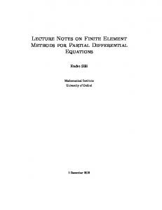
-3 3 2 1 -1 -2
KdV 1-st order dynamics Solutions of the equation F = 0; has the form u=
12} (x + c; g2 ; g3 )
a2 3
where } (x; g2 ; g3 ) is the Weierstrass elliptic function with invariants g2 =
a22
3a1 27a0 9a1 a2 + 2a32 ; g3 = : 108 11664
The shift of these solutions along X leads us to the following solutions of the KdV equation u (x; t) =
12} x
a2 t + c; g2 ; g3 3
20
a2 : 3
-2 3 2 1 -1
The solution space These pictures show the solution space and a trajectory for 1-st order dynamics with F = p31 + (p0 1)(p0 2)(p0 3): 80 6 4 u 3 2 1 0 t x
The trajectory
3.2
Second Order Dynamics
Here we describe the second order dynamics. We shall consider dynamics F (p0 ; p1 ; p2 ) = 0 which are invariant with respect to the scale symmetry xpx + 3tpt + 2p0 for KdV equation. We assign for p0 weight 2 , p1 weight 3 and p2 weight 4 and assume that F is a sum of homogeneous polynomial of degree n . The following list gives non-trivial homogeneous dynamics for small n : n=4 F4 = p20 + 2p2 + ap0 + b; 21
n=6 F6 = 2(a + 3p0 )p2
6p21 + p30 + 3ap20 + b p0 + c;
n=8 F8 = p40 =4 + p20 p2 + p22 + a(2p30
3p21 + 6p0 p2 ) + b(p20 + 2p2 ) + c
where a; b and c are constants, and n = 10 F10 = 8p32 + 9p41 : Note that dynamics F4 and F6 coincide with q10 and q11 : The previous di¤erential equation EJT gives us the following dynamics: 4096 3 512 3 2 8192 3 2 c c p0 c1 c2 p0 + c p 3 1 2 3 9 2 0 256 3 3 128 2 3 16 2 4 56 2 4 4 1 2 6 c c2 p c1 c2 p0 c c2 p + c p c1 c2 p50 + c p + 27 1 0 27 9 1 0 81 2 0 81 729 1 0 7 8 6 5c1 p0 25p0 256 3 2 640 2 2 32 2 5c2 p0 + + + c c2 p c1 c2 p1 c p0 p21 1458 17496 1679616 9 1 1 9 27 2 8 2 2 3 2 2 19c1 p40 p21 19p50 p21 1 c1 c2 p20 p21 + c1 p0 p1 + c2 p30 p21 + + + c21 p41 27 243 81 5832 69984 81 4 1 5p20 p41 32 8 1 c2 p41 c1 p0 p41 c1 c2 p21 p2 + c2 p0 p21 p2 + c1 p20 p21 p2 + 81 486 11664 27 81 81 1 4 64 2 2 32 2 2 16 2 5p30 p21 p2 2 p p2 + c1 c2 p2 c p + c1 c2 p0 p2 c2 p20 p22 2916 972 1 9 9 2 2 27 81 1 5p40 p22 1 5p0 p21 p22 p4 128 2 c1 p30 p22 + c1 p21 p22 + + 2 + p Q20 486 23328 162 1944 1296 9 1 1024 128 32 4096c21 c2 Q21 + 2048c22 Q21 c1 c2 p0 Q21 + c2 p20 Q21 + c1 p30 Q21 + 3 9 27 10 4 32 8 8 p Q21 c1 p21 Q21 p0 p21 Q21 p2 Q21 + 256Q221 + 4096c31 c2 Q22 81 0 9 27 9 2 512 2 128 32 2 3 2048 2 c c2 p0 Q22 c p0 Q22 + c1 c2 p20 Q22 c p Q22 2048c1 c22 Q22 + 3 1 3 2 9 27 1 0 32 2 5 5 32 64 c1 p40 Q22 p Q22 + c21 p21 Q22 c2 p21 Q22 c2 p30 Q22 27 9 486 0 9 9 4 2 2 4 2 8 2 p p Q22 p p2 Q22 + c1 p22 Q22 + p0 p22 Q22 512c1 Q21 Q22 81 0 1 27 1 9 27 128 128 16 p0 Q21 Q22 + 256c21 Q222 + c1 p0 Q222 + p20 Q222 = 0 3 3 9 Let’s look at the dynamics in more details. 16384c41 c22
3.2.1
16384c21 c32 + 4096c42 +
F4 = p20 + 2p2 + ap0 + b
In this case vector …eld
2 aX
V = p1
is the restriction of the vector …eld
@ @ + p2 @p0 @p1 22
(a + 2p0 ) p1 @ 2 @p2
on the zero level F4 = 0; and X can be integrated in the same way as for 1-st order dynamics. Trajectories of X are given by formulae p0 (t) = where
12} (t + K; g2 ; g3 )
a=2
12ab a3 12ab 12c2 ; g3 = 48 1738 and the constant can be found from initial data. These formulas lead us to the following pathes in the solution space g2 =
a2
u (t; x) =
12} t
ax + const; g2 ; g3 2
a=2
with arbitrary invariant g3 and g2 given above. F6 = 2(a + 3p0 )p2
3.2.2
6p21 + p30 + ap20 + b p0 + c
Di¤erential equation E = F6 1 (0) has singular points at p0 = p21 =
a ; 3 a3 81
ab c + : 18 6
Moreover, in this case symmetries Xp1 and X are linear dependent on the di¤erential equation E and X =
H p1
where H=
6p2 @ + 1 @p0
p30 ap20 bp0 2 (a + 3p0 )
ab + 3c + 6bp0
6p30
c @ @p1
;
18p21
2
2 (a + 3p0 )
is the …st integral for E; and for vector …led X : X (H) = 0 on E: Vector …eld X has also singularities at the points where a + 3p0 6= 0; and p30 + ap20 + bp0 + c = 0; p1 = 0: Depending on roots of polynomial p30 + ap20 + bp0 + c we have the following three types of phase portraits: Three real distinct roots. In the following picture we take roots: and F6 = 2 (3p0 2) p2 6p21 + p30 2p20 p0 + 2 23
1; 1; 2;
-0 8 6 4 2 -2 -4 -6 1 5 -5 10
A real root of multiplicity 2: In the picture we take roots: 1; 1; 2; and 6p21 + p30
F6 = 2 (3p0 + 4) p2
24
4p20 + 5p0
2
-0 4 2 -2 1 5 -5 10
Two complex roots. In the picture we take roots: 1; and F61 = 6p0 p2 6p21 + p30 1
25
p 1+ 3 ; 2
1
p 2
3
;
-.5 4 2 -2 -4 7 5 2.5 -2.5 -5 7.5
Solutions of the equation F6 1 (0) one can …nd from the …rst integral H: So they are solutions of the following 1-st order ODE p21 =
p30 3
kp20 +
b
2ak ab + 3c 2a2 k p0 + 3 18
for some constant k; H = k: Thus solutions of the ODE can be represented in terms of the Weierstrass function as follows u (x) = 12} (x + C0 ; g2 ; g) k where k (b + k 2ak) ; 12 12k 3 12ak 2 + 2 a2 + 3b k g3 = 2592 g2 =
ab
Note that along X function H is constant and X = corresponding path in the solution space is u (x; t) =
3.3
F = 6 (p0
) p2
12} (x
kt + C0 ; g2 ; g3 )
6p21 + (p0
c
:
HXp1 .Therefore the k:
)3
This the special case when the polynomial p30 + ap20 + bp0 + c has root of multiplicity 3: Without loss of generality we can assume that = 0; and investigate the ordinary di¤erential equation E, where F = 6p0 p2
6p21 + p30 = 0: 26
Vector …eld X on E is proportional to Xp1 X = with H=
H Xp1 p30 + 3p21 : 3p20
Where H is a …rst integral for ordinary di¤erential equation E and for the vector …eld X : -.5 3 2 1 -1 -2 -3 7 5 2.5 -2.5 -5 7.5
The ODE E can be solved directly and one gets u (x) =
a2 cosh2
Restriction of H on these solutions gives path is the solitary wave solution u (x; t) =
a(x+b) p 2 3
:
a2 =3; and therefore the corresponding a2
cosh2
27
a(x+a2 t=3+b) p 2 3
:
14 8 6 -4 t u 40 x 4 2 0 -2 0
3.3.1
F10 = 8p32 + 9p41
In this case the vector …eld X on F101 (0) is proportional Xp1 : X = with H=
HXp1
3p21
2p0 p2 : 2p2
Solutions of the equation F10 = 0 has the form 12
u (x) = B
2;
(x + A)
and H = B for these solutions. Therefore the corresponding path has the form of the rational solution u (x; t) = B 3.3.2
12 (x + A
2:
Bt)
Trivial dynamics
The following ODEs 2p30
3p21 + 6p0 p2 + a(p20 + 2p2 ) + b;
p40 =4 + p20 p2 + p22 + a(2p30
3p21 + 6p0 p2 ) + b(p20 + 2p2 ) + c;
p40 =4 + p20 p2 + p22 + a(2p30
3p21 + 6p0 p2 )(p20 + 2p2 ) + c
give the trivial dynamics: X = 0 on E-s.
28
3.4
Third Order Dynamics
The following dynamics represent non trivial polynomial dynamics in degree 10 : 1 F1 = ap1 + b(p0 p1 + p3 ) + p20 p1 p1 p2 + p0 p3 ; 2 F2 = p23 + 2p21 p2 a(p3 + p0 p1 )2 ; F3 = (p3 + p1 p0 + a) (p1 + bp0 + c) where a; b; c are constants. 3.4.1
Dynamics for F1 = ap1 + b(p0 p1 + p3 ) + 12 p20 p1
p1 p2 + p0 p3
In this case X = H Xp1 ; where H=
2p2 + p20 2a 2 (b + p0 )
is a …rst integral of ordinary di¤erential equation F1 1 (0) : Solutions of ordinary di¤erential equations H = c; where c is a constant, or p20 + cp0 + a + bc 2
p2 =
can be expressed in terms of the Weierstrass functions: u=
12} (x + c1 ; g2 ; g3 )
c
with arbitrary g3 and
3b) c2 3ac : 12 The corresponding pathes in the solution space are g2 =
u (x; t) = 3.4.2
(1
12} (x + ct + c1 ; g2 ; g3 )
Dynamics for F2 = p23 + 2p21 p2
c:
a(p3 + p0 p1 )2
Let a 6= 1; then X = H Xp1 ; where p p0 ap20 + 2 (1 H= 1 a
a) p2
is a …rst integral of ordinary di¤erential equation F2 1 (0) : Solutions of ordinary di¤erential equations H = c; where c is a constant, p2 =
p20 2
cp0 + c2 (1
29
a)
can be expressed in terms of the Weierstrass functions: u = 12} (x + c1 ; g2 ; g3 ) + c with arbitrary g3 and
c2 c3 (1 a) + : 12 2 The corresponding pathes in the solution space are g2 =
u (x; t) = 12} (x + ct + c1 ; g2 ; g3 ) + c: In the case a = 1; we have F2 = p21 2p2 and X = H Xp1 ; where H=
p20
2p0 p1 p3
p20 + 2p2 2p0
is a …rst integral of ODE F2 1 (0) : Solutions of ODEs H = c; where c is a constant, p2 =
p20 + cp0 2
can be expressed in terms of the Weierstrass functions: u=
12} (x + c1 ; g2 ; g3 )
c
with arbitrary g3 and
c2 : 12 The corresponding pathes in the solution space are g2 =
u (x; t) =
3.5
12} (x + ct + c1 ; g2 ; g3 )
c:
Fourth order dynamics
Fourth order dynamics are de…ned by functions F = p4 +
5p0 p2 5p2 5p3 p2 + 1 + 0 + a p2 + 0 3 6 18 2
+ bp0 + c
where a; b; c are constants. It is easy to check that the vector …eld X and the ODE F following …rst integral H1 =
36bp20
12ap30
5p40
12p0 6c + 5p21 + 36 6ac
30
1
ap21 + p22
(0) has the 2p1 p3 ;
and the restriction on H1 = k admits …rst integral H2 = 72 2a2 + 5b p60 + 120ap70 + 25p80 + 24p50 36ab + 30c + 19p21 + 432p41 3a2 216ac + k 72p20 +24p0
+2p40 648b2 2 36p22 24p30 216p21 72 a2 72 (3ab
36ap41 + 6c
c) c
216ac + 5k + 216 a2
b c
+ 2b c
ak
bk +
216ac + k
684ap21
180p22
ak + 36ap22
+ 12p21 3a2 + 9b + 10p2
12p2 (4c + ap2 )
10p41
+ 36bp22 36p22 + p21
12p21 (3ab + 4c + 6ap2 ) (432ac
k + 36p2 (12b + 5p2 )) :
The last ordinary di¤erential equation H2 = k2 has two symmetries X and Xp1 and they are independent and commute. Therefore the di¤erential equation can be integrated in quadratures. Namely, the method discussed above gives two 1-forms 0
1
=
p2 dp0
p1 dp1
G A dp0 + B dp1 = G
; dx;
where 1 5 p31 3acp2 kp2 cp0 p2 G = cp1 + bp0 p1 + ap20 p1 + p30 p1 + 2 18 6 p1 72p1 p1 3 4 3 ap0 p2 5p0 p2 1 5 p + ap1 p2 + p0 p1 p2 + 2 ; 6p1 72p1 2 6 2p1 p2 1 A = c + bp0 + a p2 + 0 + 5p30 3p21 + 12p0 p2 ; 2 18 k cp0 bp20 ap30 5p40 ap1 p0 p1 p2 3ac B= + + 2 ; p1 72p1 p1 2p1 6p1 72p1 2 6 2p1
bp20 p2 2p1
and integrals I0 (p0 ; p1 ) ; I1 (p0 ; p1 ) such that p2 dp0 G A dI1 = dp0 + G
dI0 =
p1 dp1 ; G B dp1 ; G
and solutions can be found from I0 = c0 ; I1 = x + c1 for some constants c0 ; c1 :
References [1] Duzhin S.V., Lychagin V.V. Symmetries of distributions and quadrature of ordinary di¤erential equations, Acta Appl. Math. 24,(1991), no.1, p.29-57 31
12b
4p2
[2] Ibragimov Nail H., Transformation groups in mathematical physics, M. Nauka, 1983 [3] Lax P.D. Integrals of nonlinearequations of evolution and solitary waves. Comm. Pure and Appl. Math., 1968, v.21, p. 467-490 [4] Gardner C.S. Greene J.M., Kruskal M.D., Miura R.M., Kortweg- de Vries equation and generalizations, VI, Methods for exact solution, Comm. Pure and Appl. Math., 1974, v.27, p. 97-133 [5] Krasilshchik I.S., Lychagin V.V., Vinogradov A.M., Geometry of jet spaces and non-linear di¤erential equations, Gordon and Breach, 1986 [6] Kruglikov Boris , Lychagin Valentin, Mayer brackets and solvability PDEs,1, Di¤. Geometry and Appl., 17 (2002), p.251-272 [7] Abramowitz M., Stegun I.A., Handbook of Mathematical Functions, Dover, 1972
32