Finite element models in electrical machine design

Finite element models in electrical machine design K. Hameyer, F. Henrotte, Hans Vande Sande, Geoffrey Deliège, Herbert De Gersem Katholieke Universiteit Leuven EE dept. ESAT / ELECTA Kasteelpark Arenberg 10, B-3001 Leuven – Heverlee

Abstract — In the last thirty years, ongoing and fast developments of numerical techniques for the particular questions concerning electrical machinery can be noticed. This development can be seen in parallel with the efforts and success of the soft- and hardware computer industry in producing powerful tools. Computers as well as the commercial software are now ready to be applied to solve realistic numerical models of technical relevance. Of course, there are enough complicated problems and questions, which are not yet answered to a satisfactory extend. This paper is intended to focus on special problems concerned to better solution of electrical machine design and simulation questions. Particular attention is given to the topics of material modeling, winding and coil models and to the dynamic simulation of electrical machinery. Today, efficient numerical solutions can be obtained for a wide range of problems beyond the scope of analytical methods. In particular the limitations imposed by the analytical methods, their restrictions to homogeneous, linear and steady state problems can be overcome using numerical methods. INTRODUCTION At the time, when not too many computers where available yet, the design of electrical machines was performed in the classical way, by using onedimensional models. Particular electro magnetic parts of the machine are considered to form a homogenous element in a magnetic circuit approach. In this approach the knowledge of particular “design” factors is assumed. Such models enabled the calculation of specific stationary working points of the machine. Laplace transformations applied to such models made it possible to analyze the machine for the dynamic operation. The refinements of the 1D models yield the technique of magnetic equivalent circuit models.

A very rough figure can be drawn in saying that the development of numerical methods for electrical machines started with the finite difference method which quickly was followed and further overtaken from the finite element method. With the first numerical models of electrical machines, in the 70s, electromagnetic fields considering imposed current sources could be simulated by applying first order triangular elements [1]. Further developments of the finite element method lead via the definition of external circuits to problem formulations with imposed voltage sources, which where more accurate models with respect to the realistic machine that is operated by a voltage. Today’s developments are directed to all aspects of coupled fields. There are the thermal/magnetic problems or structure dynamic field problems coupled to the electromagnetic field; e.g. acoustic noise in transformers and rotating machines excited by electromagnetic forces. Parallel with the developments of the finite element method first attempts to numerically optimise the finite element models where made. Optimisations of realistic machine models where first performed in the late 80s and early 90s. Various deterministic and heuristic methods have been applied and can be found in the conference proceedings e.g. COMPUMAG and CEFC of that time. Research groups at universities have code available that goes further in modeling. For example, it can consider external electrical circuits with power electronic components operating the machine model. Such models are consuming a lot of computational time. However, research directed to accelerate the numerical solvers is going on as well. Extensions of the overall machine models can be made by applying more realistic material models. Hystersis effects and material anisotropy are still a lack in many software packages. Special winding models allow to reduce the size of a numerical model significantly and therefore the computation time as well. To avoid long lasting transient simulations single-phase machines can be modelled by a time-harmonic approach by modelling separate

rotor models for the rotary fields in reverse respectively rotation direction of the rotor. However, with all developments of numerical techniques around the electrical machine analysis, it must be noticed that the classical approach can not be replaced by the numerical models. Enormous expertise and knowledge to model the various electromagnetic effects appropriate and accurately is still required. The modeling/solving/postprocessing of numerical motor models still requires substantial engineering time and can not replace the quick and correct answer of an exercised motor design engineer. Both experts, probably in one person, numerical modeling and electromagnetic motor design engineer, are required for successful and novel developments in this engineering discipline. FINITE ELEMENT MODELS It all starts with Maxwell’s equations (Table I). Every electromagnetic phenomenon can be attributed to the seven basic equations, the four Maxwell equations of the electrodynamic and those equations of the materials. The latter can be isotropic or an-isotropic, linear or non-linear, homogenous or non-homogenous. Table I. Maxwell’s equations. differential form

(i) (ii) (iii) (iv)

integral form

∂B ∇×E= − ∂t ∇ ×H = J

dφ

D, B , H, and J and the space charge density ρ are in general functions of time and space. The conducting current density can be distinguished by a material/field dependent part J c and by an impressed and given value J0 . It is assumed that the physical properties of the material’s permitivity ε, permeability µ and conductivity σ are independent of the time. Furthermore it is assumed that those quantities are piecewise homogenous. The Maxwell equations represent the physical properties of the fields. To solve them, mainly the differential form of the equations and mathematical functions, the potentials, satisfying the Maxwell equations, are used. The proper choice of a potential depends on the type of field problem. The electric vector potential for the displacement current density will not be introduced here, because it is only important for the calculation of fields in charge-free and current-free regions such as hollow wave-guides or in surrounding fields of antennas. Various potential formulations are possible for the different field types. Their appropriate definition ensures the accurate transition of the field problem between continuous and discrete space. Using these artificial field quantities reduces the number of differential equations. Considering a problem described by n differential equations, a potential is chosen in such a way that one of the differential equations is fulfilled. This potential is substituted in all other differential equations, the resulting system of differential equations reduces to n-1 equations.

∫ E ⋅ dr = − dt

Flux

C

∫ H ⋅ dr = I

Coil

C

∇⋅ B = 0

∫ B ⋅ dS = 0

Movement

S

∇⋅ D = ρ

∫ D ⋅ dS = Q S

(v)

B = µH

(vi)

D = εE

(vii)

J = J 0 + J c = J 0 + σE

The Maxwell equations are linked by interface conditions. Together with the material equations they form the complete set of equations describing the fields completely. φ is the magnetic flux, I the conducted current, Q the charge, C indicates the contour integral and S the surface integral. The seven equations describe the behavior of the electromagnetic field in every point of a field domain. All electric and magnetic field vectors E,

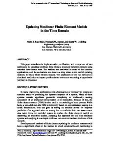
Fig. 1. (top) Geometry, direction of movement, expected flux path and (below) the associated 3D FEM discretisation of a linear transversal flux (TF) motor. (the surrounding discretized air is not plotted)

To build up a FEM model, in a pre-process the device’s geometrical shape is approximated by finite elements. In two-dimensional models the standard elements are commonly triangles and in the three-dimensional case tetrahedron elements can be used. This type of elements is very flexible and capable to approximate very well even complicated geometrical shapes (Fig. 1). In this step of modelling the device, material and boundary conditions have to be defined. Outgoing from the computed potential solution, the interesting field values, such as field strength and magnetic flux density can be calculated for all places inside the model. From the obtained field values e.g. the forces and other physical quantities, such as the induced currents and voltages can be derived. Computer models enable a thorough study of actuators without the requirement of expensive prototyping. Prototyping is of course required at the end of the design procedure to verify simulated results or if required to improve the device’s numerical model. Various different geometrical variants of an actuator concept can be studied and the particular properties can be compared. Figure 2 shows two different variants of a concept of a linear TF actuator with their associated force characteristic.

utilisation of the materials used. The recent developments and ongoing research in the field of hard- and soft-magnetic material delivered materials with improved material properties (Fig. 3). Therefore, extremely small electric motors with very compact electromagnetic circuits can be developed (Fig’s. 4 and 5) by applying appropriate and accurate material models. 1000 3

kJ / m 900

(BH)max.theor. = 960 kJ / m³ theoretical

800 (BH)max. 75 % = 720 kJ / m³ technically possible

700 600 500 (BH)max / 2

400 NdFeB

300 Sm2Co17

200 AlNiCo

100

SmCo5

Steel Ferrit

0 1880 1900 1920 1940 1960 1980 2000 2020 2040 2060 2080

Year

Fig. 3. Development of permanent magnet material. (source: VACUUMSCHMELZE , Germany)

10

¹ Net force (in N)

5

0

¶

-5

· ¸

-10 0

0,2

0,4

0,6

0,8

1

Position (in # pole pitches)

Fig. 2. 3D FEM models of variants of a TF linear motor with the associated force vs. position characteristic.

SPECIAL MATERIAL MODELLING The ongoing trend towards the miniaturisation of systems and the trend of system integration force the development engineers to construct smaller and smaller devices. Key here is the appropriate

¹ ¶ stator · permanent magnet system ¸ rotor ¹ winding

Fig. 4. Magnetic field solution of a small electromagnetic stepper motor excited by novel rare earth permanent magnet material.

For the analysis of electrical machines usually a 2D-FEM electrodynamic model is built which lies in the plane of the flux. For this case, no eddy currents in the x-plane of the lamination (Fig.6) can be considered. To cope with this problem the model has to be built in the xy-plane, where the flux then is perpendicular to it. To realize a solution for this model, an electrodynamic “in-plane” formulation using the electric vector potential T is chosen: ∇ ×T = J ,

(1)

this yields the time-harmonic formulation −

Fig. 5. Three members of the Penny-Motor family: a) HE type for high torque; b) YL type for low price; c) EC type for electronic commutation. (source: mymotors & actuators gmbh, Germany)

A. EDDY CURRENTS IN LAMINATED FERRO-MAGNETIC ELECTRIC STEEL High permeable steel laminations are usually used for the design of the magnetic core of electrical machines. This is because of its magnetically good properties. However, the material is electrically very good conducting as well. As a consequece eddy current losses have to be considered in the model of steel lamination when time varying fields have to be assumed. To lower the eddy current losses in AC fields several iron laminates with coating material on both surfaces are applied. The coating material is less conductive and less permeable when compared to the iron. This prevents excessive eddy current losses but at the expense of a higher reluctance of the global magnetic flux path [2] (Fig. 6). lz

(µ1, σ1 )

lx

(2)

ρ is the resistivity, µ the permeability, jω is the angular frequency, Vm the magnetomotive force and lz the length of the problem in z-direction. With this model it possible to determine the losses for single sheets and for multiple layer arrangements of ferromagnetic lamination (Fig.7). For the simulation of multiple layers an FEM approach with external magnetic circuits for the flux in z-direction has to be chosen [3].

Rm

Fig. 7. 2D electrodynamic model of a laminated material of various layers combined with a magnetic equivalent circuit [3].

φz J

δ

∂  ∂T z  V ρ  + jωµT z = − jωµ m . ∂x  ∂x  lz

(µ2 ,σ2 )

Fig. 6. One sheet of ferromagnetic lamination with coated surfaces.

Semi-analytical simulations consider the losses in a single laminate and neglect the conductivity and permeability of the coating material. The model presented here deals with coating material with a finite resistivity. As a consequence, the closing path of the current may cross the coating layers. The eddy current losses are completely different from the simplified analytical model. As an external condition, the total magnetic flux through the model has to equal the applied flux. The magnetic

equivalent circuit represents the parallel connection of all domains in the electrodynamic model, excited by a flux source (Fig.7). By using this hybrid modelization technique, the coupled FEM and magnetic equivalent circuit model, dependencies of the eddy current losses can be studied with respect to the frequency and the number of iron layers (Fig. 8a, b, c). The results can be employed to simulate the materials behavior in electrical machines for various frequencies. To consider the complicated shape of e.g. an induction machine these simulated results have to be transformed in such a way that they can be used in the 2D model of a realistic electrical machine.

some fixed directions. The reluctivity ν meas [Am/Vs] H νmeas = meas , (3) Bmeas depends non-linearly on Bmeas. Fig. 9 shows the measured reluctivity curves for a conventional grain-oriented (CGO) steel, along several directions with respect to the rolling direction [4, 5].

RD

54.7 °

TD

Fig. 9. Definition of the Goss-tecture with rolling direction (RD) and transverse direction (TD). a)

b)

1500 Re luc 1200 tivi 900 ty [A 600 m/ Vs 300 ] 0

70 40 90 50 30 20 60 80 10 0

0.0 c)

Fig. 8. Eddy current density distribution for a field at a) 50 Hz, b) at 500 Hz and c) voor comparison, multiple laminations at a frequency of 50 Hz [3].

B. FERROMAGNETIC ANISOTROPY Grain-oriented ferromagnetic materials exhibit anisotropy at both the microscopic and the macroscopic level. In order to assess the macroscopic anisotropy of these materials, single sheet testers are often used. This is done by measuring the magnetization curve Bmeas (H meas ) of a series of small strips, cut out of a metal sheet under various angles. As single sheet testers can only perform unidirectional measurements, these magnetization curves represent a relation between the components of the magnetic flux density B [T] and the magnetic field strength H [A/m] along

0.4

0.8

1.2

1.6

2.0

2

Flux density B [Vs/m ]

Fig. 10. Reluctivity curves for grain-oriented steel under various angles referencing to the RD.

However, for anisotropic ferromagnetic materials, the vectors representing the magnetic field and the flux density are not parallel with each other. It is impossible to deduce the angle between B and H, by exclusively considering the measured magnetization curves. For ferromagnetic materials having a Goss-texture, like most transformer steels, the paper demonstrates a way to compute this angle a posteriori, by combining the measurements from a single sheet tester with a physical anisotropy model. r The magnetization Ms [A/m] within a domain tends to align with one of the easy axes of the crystal. Each deviation from this equilibrium state

corresponds to an increase of energy, which is due to the intrinsic anisotropy of the crystal. For cubic crystals, the anisotropy energy Ea [J/m3 ] is given b:

field, an expression for the amplitude of M is obtained:

Ea = K 0 + K 1 (γ12γ 22 + γ 22γ 32 + γ 32γ12 ) + K 2 (γ12γ 22γ32 ) (4)

(7)

M = (Bmeas / µ0 − H ) / cos(α − θ) .

r

with γ1 ,γ2 and γ3 the direction cosines of Ms in the crystallographic coordinate system [4]. K0 is an arbitrary constant. K1 and K2 are the anisotropy constants. In case of a cubic iron crystal, these are K1 = 0.48⋅105 J/m3 and K2 = 0.05⋅105 J/m3 [5]. On r the other hand, if an external field H is applied, r Ms tends to align with it. The corresponding energy Eh [J/m3 ] is the so-called field energy

r r Eh = −µ0 M s ⋅ H .

(5)

RD M ?

B / µ0

ß a

H

Bmeas / µ0

Fig. 11. Definitions within the measurement set-up.

The process of coherent rotation of the domains can be considered as a competition between the r anisotropy energy (2) and the field energy (3): Ms stabilizes in a direction for which the total energy is minimal.

Subsequently, the components of B are obtained by projecting (6) on the RD and the TD:

For silicon iron having a Goss-texture, (2) and (3) simplify into

Using the previously presented hybrid approach, it is possible to compute the two components of B and hence the reluctivity tensor. If this symmetrical second order tensor is considered in its principal coordinate system, it has zero off-diagonal entries [6]. For this application, the RD and the TD are the principal axes of the tensor, as B and H are parallel in these directions. As a consequence

Ea =

K1 sin 2 θ (4 − 3 sin 2 θ ) 4

(6)

and Eh = − µ0 M sH cos(α − θ )

(7)

 B / µ0 cos β = H cos α + M cos θ   B / µ0 sin β = H sin α + M sin θ

,

(8)

r

with α the angle between the field H and the RD, r and θ the angle between Ms and the RD. After evaluating (6) obviously, θ = 54.7 ° corresponds to a maximum of Ea. Hybrid Model. The hybrid method works in two steps. The direction of the magnetization M is first determined for a fixed direction of H, by means of the previous discussion. If α < 54.7 °, the minimum of Ea + Eh at low values of θ is determined. Else, the minimum for high values of θ is determined. The second step consists in extracting the amplitude of M, knowing its direction, from the single strip tester measurements (Fig. 11). This is done as follows. The flux density B is related to the applied field H and the magnetization M by:

(

r r v B = µ0 H + M

)

(8)

The measured and applied field strength are equal. By projecting (8) onto the direction á of the applied

 H RD  νRD 0  BRD    =    ,  H TD   0 νTD  BTD 

(9)

with νRD = ( H cosα) / (B cos β) and

νTD = (H sin α) /(B sin β )

(10)

for the specified measurement point with β the angle between B and the RD. The hybrid model is analyzed for the data set plotted in Fig. 12. It can be shown, that for low fields H, the flux density vector stays close to the RD or the TD, irrespective of the field direction α. On the other hand, for very higher fields (> 1,7 T), H and B tend to align. This is in correspondence with the theory of magnetization [7,8,9]. Fig. 13 reveals how the field behaves, if the flux density

rotates in space with constant amplitude. The result, for |B| = 1.7 T is plotted in Fig. 14.

Fig. 12: The magnetization curves applied to explain the model.

H↑

SIMULATION OF THE TRANSIENT SYSTEMBEHAVIOR BY STAGED MODELING This section presents a methodology to achieve an overall model of a power system that consists of a battery, an inverter, a permanent magnet servomotor and a turbine. Particular attention is paid to the fact that one single finite element model would not be able to provide a satisfactory representation of the behavior of the overall system. A staged modeling is proposed instead, which succeeds in providing a complete picture of the system and which relies on numerous finite element computations. The key point in the realization of a staged model is to define carefully the interface quantities between the different components of the system. Between the inverter and the motor, the interfacing quantities are the electrical quantities associated with the three stator phases. In particular, to represent the back-emf of the phase, we will pay attention to the flux distribution: φ(Θ, I ) =

r

∫ b(Θ, I ) ⋅ ndS

(11)

S ph

α↑

H↑

Fig. 13. B and β as a function of H (data set fig. 12).

B H

which gives the total flux embraced by one stator phase as a function of the angular position of the rotor Θ and the current in that phase I. If the motor works in steady state operation, the flux distribution of one phase is sufficient, as the flux plot for the other phases are obtained by a simple angle shift. If the machine works in a non-saturated state, the dependence on I can be neglected. The flux plot gathers in one table all the required information concerning the motor, seen from the inverter. At high motor-speeds respectively high supply frequencies, iron core losses may override copper losses and have therefore to be estimated carefully over a wide range of frequencies. A difficulty in the calculation of core losses is that the magnetic flux density not only varies in time but also varies widely in space. Usually one distinguishes hysteresis losses, which are proportional to the frequency and eddy current losses, which are approximately proportional to the square of the frequency. One will therefore assume that core losses can be expressed by the formula Q core( I , ω) = C1 ( I )ω + C 2 ( I )ω2

Fig. 14. H-locus when B rotates at 1,7 T (data set fig. 12).

(12)

where the frequency independent constants Cl (I) and C2 (I) are expressed by:

C1 ( I ) =

 2π

∫  ∫ h∂

core

0

 b ( Θ, I ) d Θ , 

 Ceddy 2π  2 C 2 ( I ) =  ∂ Θ b (Θ, I ) d Θ  2π 0 core 

∫

table II, which considers the various switching states of the inverter.

Θ

(13)

∫

This assumption is one of the simplifications of the staged modeling. It can be seen that the flux distribution (11) as well as the core losses parameters (13) depend on b(Θ, I ) and ∂ Θ b (Θ, I ) . They can therefore be computed beforehand for a given geometry of the motor, by post-processing adequately a series of 2D static FE computations, and then storing the results into look-up tables. Because of the large difference in scale between one electrical period and the time required for the motor to reach its steady state operation, a classical transient analysis would require several tenthousands of time steps. The transient analysis is therefore split-up into two parts. The first part consists in calculating 'over one period' the stationary current wave shapes for a fixed speed ω , a fixed commutation angle α and fixed operation temperature. The second part is the transient dynamic and thermal analysis. This splitting is one of the simplifications of the staged modeling. During the 'over one period stationary' analysis, the inductances , resistances and back-emf's of the phases, the extra voltages and resistances due to the electronic components and the switching strategy of the inverter bridge are all considered for the computation of the wave shapes of the phase currents and voltages. One starts from the voltage equation of one stator phase: Vξ = Rξ I ξ + ∂ tφξ , with index ξ = A, B, C

(14)

in which the flux coupling φξ is given by (11). The total resistance of the phase is computed analytically and can be augmented by an extra resistance due to the power electronic components. The total phase voltage Vξ is equal to the power electronic inverter’s dc-link voltage V dc dis tributed over the different phases, according to the particular topology at each instant of time of the inverter and to the winding connection type, deta respectively Y-connection. In this example we consider a Y-connection and it can be written: Vξ = λ ⋅ Vdc

(15)

λ is the coefficient, which can be taken from the

Table II. Coefficient for the distribution of the dc-link voltage to the three winding phases A, B, C. Phase A

Phase B

Phase C

0 1/2 -1/3 1/3

OFF OFF 2/3 1/3

0 -1/2 -1/3 -2/3

+1 → 0

0 → +1

− 1 → −1

OFF OFF -2/3 -1/3

0 1/2 1/3 2/3

0 -1/2 1/3 -1/3

0 → −1

+ 1 → +1

−1 → 0

0 -1/2 -1/3 -2/3

0 1/2 -1/3 1/3

OFF OFF 2/3 1/3

− 1 → −1

+1 → 0

0 → +1

0 -1/2 1/3 -1/3

OFF OFF -2/3 -1/3

0 1/2 1/3 2/3

−1 → 0

0 → −1

+ 1 → +1

OFF OFF 2/3 1/3

0 -1/2 -1/3 -2/3

0 1/2 -1/3 1/3

0 → +1

0 → −1

+ 1 → +1

0 1/2 1/3 2/3

0 -1/2 1/3 -1/3

OFF OFF -2/3 -1/3

+ 1 → +1

−1 → 0

0 → −1

The table consists of six sections, which correspond to the six periods between the switching-on of two successive phase windings. For instance, let us consider the last group of four lines in the table. In the considered period, the phase A has to be switched on ( 0 → +1 ) and the phase C has to be switched off ( + 1 → 0 ), the phase B remains in the same state as before ( − 1 → −1 ). Immediately after sending the switch-on signal to phase A, all three phases are magnetized by its corresponding currents. The inverter topologies corresponding with the last two lines of the group of the table are used then. In both states, the voltage is positive in the switched-on phase (i.e. phase A), the voltage is negative in the switched-off phase (i.e. phase C), and the voltage is either positive or negative in phase B, which allows to control the current in that phase. After a while, the current in phase C reaches

zero and the phase ceases to be conducting. From that instant on, the first two lines of the group are applied, the first one to let the current decrease (freewheeling) and the second one to make it increase in the loop formed by the phases A and B. Outgoing from the voltage equation (14) the explicit time-stepping scheme for the phasecurrents can be derived: I ξ ( Θ + ∆Θ) = I ξ ( Θ) +

Vξ − ω∂ Θφξ − Rξ I ξ ( Θ) ω∂ I φξ

∆Θ

(16) The given scheme can be applied until the steady state of the transient behavior, the steady state wave-shapes of the currents I ξ (Θ) over a period τ

a)

is reached. With this, the electromagnetic torque can be evaluated: 2π

3 Q ( I , ω) − ∂ Θφ(Θ − α) I ( Θ)d Θ − core 2π 0 ω (17) In a following step the dynamic differential equation of motion is applied to form the transient analysis of the overall drive system. T (ω,α) =

∫

J∂ tω + f (ω) = T (ω, α) ,

b) (18)

where J is the inertia of the rotating part, f (ω ) is the reaction torque exerted by the load and friction forces. When temperature-sensible devices, such as e.g. permanent magnet excited systems are studied, at this point of analysis a thermal model has to be applied as well [10]. With the described modeling both, transient and steady state behavior of the drive can be analyzed for e.g. arbitrary values of the commutation angle α. However, to conclude this approach of combined analytical parameter model and numerical finite element model, building the staged model has implied assuming particulatr simplifications. On the other hand the staged model has the big advantage of providing at a reasonable computational cost a faithful dynamic and steady state description of an overall drive system. As the development goes along, the staged model is open to gradual enrichment and improvements, thanks to further FE investigations aiming at determining its different parameters or at estimating the influence of the simplifications that have been done. Fig. 16 illustrates some results obtained from a servo-motor. Flux weakening consists here in selecting, at each speed ω , the commutation angle α that maximizes the torque in that point of operation.

Fig. 15. Steady state wave-shape form of the phase current at a speed of a) ω = 1000rad / s with α = 0O and b) at ω = 2500 rad / s at α = 55O .

Fig. 16. Steady state torque of the speed and commutation angle α including the field weakening range of a permanent magnet excited servo-motor.

NUMERICAL OPTIMIZATION OF FINITE ELEMENT MODELS The design process of electromagnetic devices reflects an optimisation procedure. The construction and step by step optimisation of technical systems in practice is a trial and error-

process. This design procedure may lead to suboptimal solutions because its success and effort strongly depends on the experience of the design engineer. To avoid such individual parameters and thus to achieve faster design cycles, it is desirable to simulate the physical behaviour of the system by numerical methods such as the finite element method. In order to get an automated optimal design, numerical optimisation is recommended to achieve a well-defined optimum. Optimisation of electro-magnetic devices turns out to be a task of increasing significance in the field of electrical engineering. The term of Automated Optimal Design (AOD) describes a self-controlled numerical process in the design of technical products. Recent developments in numerical algorithms and more powerful computers offer the opportunity to attack realistic problems of technical importance. In general, the development of numerical optimization algorithms can be distinguished in their evolution into three generations: • First generation: Direct evaluation of a quality function; end 80s and early 90s. • Second generation: Evaluation of an polynomial approximation of the quality function; around 96s. • Upcoming third generation: The unknown quality function is constructed by using artificial intelligence, such as Neuro-fuzzy models. The two first generations of numerical optimization algorithms with known objective function can be distinguished in deterministic (gradient methods, linear programming) and stochastic approaches (genetic algorithms, evolution strategy, simulated annealing). A prerequisite of the deterministic approach is the availability of derivatives, which is for the optimization of FEM models mainly not the case. Their advantages can be seen in its efficient iterative search. However, such algorithms can easily be trapped in a local minimum. Stochastic search methods do not use derivatives, are robust in identifying the global optimum but have the disadvantage of very large computational costs. This can be partly overcome by searching the optimization space in parallel. A hybrid optimization can be obtained by identifying a global optimum by stochastic methods which is further evaluated by a deterministic search to extract the global minimum. These combined algorithms have the advantage of a higher accuracy and are more efficient regarding computational expenses. The distinctive feature of an electromagnetic optimisation problem is its complexity, which

results from a high number of design parameters, a complicated dependence of the quality on design parameters and various constraints. Often the direct relation of the desired quality of the technical product on the objective variables is unknown. Stochastic optimisation methods in combination with general numerical field computation techniques such as the finite element method (FEM) offer the most universal approach in AOD. To be able to select the appropriate optimisation algorithms to form an overall design tool together with the numerical field computation, the properties of typical electromagnetic optimisation problems has to be considered. Electromagnetic design and optimisation problems nowadays reflect mainly the following categories: • constrained • problem type: parameter- or static optimisation, f ( x ) → min . trajectory,

f (x&, x) → min . • •

or

dynamic

problem,

non-linear objective function design variables: real mixed real/integer • multi-objective function • interdependencies of the quality function and the design variables are unknown; no derivative information available • the quality function is disturbed by stochastic errors caused by the truncation errors of the numerical field computation method. In reality electromagnetic optimization problems are constrained due to the various reasons mentioned. Nowadays optimizations are performed mainly as static problems. Numerical optimizations require huge amounts of computation time. Therefore, the optimization as aimed at here, combined with the FEM, of the dynamic system with time-derivative x& is not yet commonly performed. For transient problems an evaluation of the quality function by numerical methods (FEM) is still too time consuming. Considering mixed real/integer design variables results in long computation times as well. The tick boxes in the list, which are not marked, represent future developments. In general, optimization means to find the best solution for a problem under the consideration of given constraints and it does not mean to select the best out of a number of given solutions. The application of an optimization using evolution strategy and the FEM is demonstrated here by the

optimization of a small dc motor applying the evolution strategy [11]. The objective is to minimise the overall material expenditure, determined by permanent magnet-, copper- and iron volume subject to a given torque of the example motor.

Z ( x)

 cos t ( x) −cos tmax      cos t max  = 10 

+ penalty → min .

(19)

The use of penalty term in the form:  Tmin −T ( x)     T < Tmin :  T ( x )  penalty =  10 T ≥ Tmin : 1 

(20)

allows the evaluation of the objective function even if the torque constraint is violated. The torque is computed by integrating the Maxwell stress tensor in the air gap region of the motor. Flux density dependent rotor iron losses were taken into account at a rated speed of 200 rpm and subtracted from the air gap torque to form the resulting output torque. The overall dimensions and the slot geometry of the DC motor are described by 15 free design parameters. The free parameters are the n/2 edges of the polygon describing the rotor slot contour and the outer dimensions of rotor and stator as indicated in Fig. 17. The motor consists of a stator back-iron with a 2-pole Ferrite permanent magnet system and a rotor with six slots. The two-dimensional field computation is employed to compute the torque of the machine to finally determine the quality function (eq.’s 19 and 20). The torque of the machine is computed, by employing the standard two-dimensional finite element analysis. To ensure controlled accuracy, adaptive mesh generation is used until a given error bound is fulfilled.

¶

·

¹ ¸ 1. stator back iron 2. permanent magnet 3. rotor iron 4. winding slot Fig. 17. Geometry definition for the shape optimization of a DC motor [11].

Fig. 18. Course of the optimization.

Fig. 19. Design variants during optimization. (# generation: quality)

The change of shape from a sub-optimal initial geometry to the final shape of the motor can be taken from Fig. 19. It can be noticed that the iron parts of the initial geometry are over dimensioned. The actual torque of this configuration was approximately 25% lower than the desired value Tmin . The optimized motor holds the torque recommended, which is achieved mainly by enlarging the winding copper volume by about 20%. The most significant change from start to final geometry can be seen in the halving of the iron volume. Consequently the iron parts are highly saturated, especially the teeth regions. In comparison to this, a test optimization with neglected rotor iron loss results in a 10% smaller rotor diameter. Unfortunately, the permanent magnet material is brittle, which limits the minimum magnet height. The magnet volume decreases slightly. Along optimization the overall volume off the motor was reduced by 38%. The rate of convergence is plotted in Fig. 18. It can be noticed, that the used evolution strategy is relatively fast converging towards the desired minimum. However, from generation 60 to the final solution no large changes can be observed.

Therefore, technically interesting results with e.g. with regard to fabrication tolerances can already be obtained in an early stadium of the optimization. DESIGN EXAMPLE: PENNY MOTOR Designed to provide an output torque of more than 100 µNm, the high-end Penny-Motor as a member of an ultra flat micro-motor family has a diameter of 12,8 mm and a height of 1,4 mm (Fig. 5). Important application fields for these innovative drives are e.g. data-com, medicine, automobiles, automation. The efficient development of such a motor is not possible without modern numerical techniques [12]. Core centre of the penny motor is a three-strand disk shaped coil produced by lithographical methods and a merely 400 µm thick magnet-ring made of rare-earth material consisting of eight segments, which correspond to four poles-pairs. Both, coil and magnet-ring decisively determine the performance of the motor. The integrated miniature ball bearing is as an option magnetically pre-stressed and therefore practically slack-free. In addition, the revolving magnetic back-iron minimizes the influence of eddy currents with the known positive effects on the motor’s efficiency (Fig. 20). A. MAGNETIC CIRCUIT OF THE PENNY-MOTOR

The main goal of dimensioning the magnetic core, was to achieve a maximum torque at a minimum of used volume. The operating point of the PennyMotor was calculated and optimized by parameter variations. The calculation includes an approximation of the stray materials, such as rare-earth permanent magnet material NdFeB (Fig. 3). Different types of soft magnetic materials where studied as well.

Fig. 20. Magnetic circuit of the HE Penny-Motor. (source: mymotors & actuators gmbh, Germany)

Fig. 21. Function of the non rotating pre-stress ring within the magnetic circuit of the Penny-Motor. (source: mymotors & actuators gmbh, Germany)

To analyse the magnetic circuit, a FEM tool was used to examine the different motor types. Verified by experiments the magnetic flux density within the air-gap of the high-end motor shows significantly more than 0,5 T. As illustrated in Fig. 20, the soft magnetic components lead the magnetic flux essentially through the ferromagnetic housing of the motor. These soft magnetic parts of the motor are optimized for a saturation of 1,6 T. This design ensures that the bearing in the inner area is not affected by magnetic fields. Fig. 21 shows the effect of the pre-stress ring. In this configuration the ring causes a well-defined magnetic force of about 0,3 N on the ball bearing. Depending on the geometry of the pre-stress ring this force can be varied in the wide range of 0 N up to more than 5 N. B. MAGNETIZING PROCESS OF RIZED NdFeB MAGNETS

MINIATU-

In the case of applying the anisotropic NdFeBmaterial the magnet-rings should be constructed of a single ring guaranteeing for its geometry of being within close tolerances. In spite of the lower magnetization energy, when compared to the compounded grades of NdFeB, the anisotropic material requires a minimum magnetic field of e.g. 2400 kA/m for 100% saturation. To ensure a uniform, magnetization within the complete magnet segment area, in practice magnetic fields up to 4000 kA/m and more must be applied to the magnets during the magnetization procedure. Because of the small magnet segments and the required high magnetic field, a specially adapted magnetization tool was developed by using the FEM [13]. The FEM analysis delivered simulation results of the magnetic field excited by high

currents. This represented a solid basis for the final design of the magnetization tool.

REFERENCES [1]

Andersen, O.W., “Transformer leakage flux program based on the finite element method,“ IEEE trans. on power apparatus and systems, PAS-92, p.p. 682-9.

[2]

P. Hahne, R. Dietz, B.Rieth, T. Weiland, IEEE Trans. Magn. 31 (1996). De Gersem, H., Hameyer, K., “Electro-dynamic Finite Element Model Coupled to a Magnetic Equivalent Circuit”, Proc. Conf. NUMELEC’2000, Potier, 2000. G.H. Shirkoohi, M.A.M. Arikat, “Anisotropic properties in high permeability grain-oriented 3.25% Si-Fe electrical steel”, IEEE Trans. on Magnetics, Vol. 30, No 2, pp 928930, March 1994. G.H. Shirkoohi, J. Liu, “A finite element method for modelling of anisotropic grain-oriented steels”, IEEE Trans. on Magnetics, Vol. 30, No 2, pp 1078-1080, March 1994. J.F. Nye, Physical Properties of Crystals. Oxford, UK, Clarendon Press, 1985.

[3]

[4]

[5]

Fig. 22. Simulation of the magnetization process. Profile of a magnetic field caused by a current of approximately 5000 A through a special shaped copper conductor within the magnet ring. (source: mymotors & actuators gmbh, Germany)

[6] [7] [8]

CONCLUSIONS [9]

Computer simulation is a powerful assistant in the field of electrical machine R&D. Decisively for success is often the combination of simulating electric, electromagnetic, thermal and mechanic phenomena’s. It is not compelling to solve this tasks with only one flexible but complex tool. In many cases of practical relevance a combination of highly specialized simu lation tools leads to qualified results. ACKNOWLEDGENMENTS The authors are grateful to the Belgian “Fonds voor Wetenschappelijk Onderzoek Vlaanderen” for its financial support of this work and the Belgian Ministry of Scientific Research for granting the IUAP.

[10]

[11]

[12]

R.M. Bozorth, Ferromagnetism. Princeton, New Jersey, D. Van Nostrand Company, 1951. D. Jiles, Introduction to Magnetism and Magnetic Materials. London, UK, Chapman & Hall, 1991. P. Robert, Traité d’Electricité, Matériaux de l’Électrotechnique. Lausanne, Switzerland, Presses Polytechniques Romandes, 1987. Henrotte F., Podoleanu I., Hameyer K.: "Staged modelling: a methodology for developing real-life power systems. Application to the transient behaviour of a PM servo motor," 15th International conference on electrical machines (ICEM), Brugge, Belgium, n° 529, August 2528, 2002. Hameyer, K., Belmans, R., Numerical modelling and design of electrical machines and devices, WIT Press, 1999. Hameyer K., Nienhaus M.: "Electromagnetic actuators current developments and examples," Proc. Conf. Actuator 2002, Bremen, Germany, (CD-Rom), 10-12 June, 2002.

[13] Kleen, S.; Ehrfeld, W.; Michel, F.; Nienhaus, M.; Stölting, H.-D.:“Penny-Motor: “A Family of Novel Ultraflat Electro magnetic Micromotors”. Actuator 2000, Bremen, 2000.