Thai Journal of Mathematics Volume 3 (2005) Number 2 : 223–240
Finite Element Solution for 1-D Groundwater Flow, Advection-Dispersion and Interphase Mass Transfer : I. Model Development M. Khebchareon and S. Saenton Abstract : Prediction of the mass transfer behavior of the entrapped dense nonaqueous phase liquid (or DNAPL) in the subsurface environment is an uneasy task. Mathematical description of this problem, which involves the solution to groundwater flow, advection-dispersion, and interphase mass transfer equations, is complex and results in a non-linear coupled system of partial differential equations where no analytical solution exists. Available, but limited, numerical tools can only solve these problems using explicit approach where all governing equations are numerically approximated as an uncoupled system of equations. This paper presents an initial development of a one-dimensional numerical solution to this problem where the system of equations is solved implicitly. Crank-Nicolson FiniteElement Galerkin (CN-FEG) scheme is developed and implemented. Assumptions are made so that the code can be compared or verified with available analytical solution. Error analysis and rate of convergence are also presented. Keywords : Finite-element, groundwater, advection, dispersion, mass transfer. 2000 Mathematics Subject Classification : 81T75, 81T80.
1
Introduction
Dense non-aqueous phase liquids (DNAPLs) such as chlorinated solvents are common organic contaminants found in subsurface environment throughout the hazardous waste sites around the world [1]. These chemicals are health hazard and some are known to be carcinogens. Once they leaked or spilled into soils, as shown in Fig. 1, significant fraction of DNAPL remained entrapped and slowly dissolve into the flowing groundwater. Partial or full exposure to polluted groundwater results in a high risk for those who are located downstream of the DNAPL source zone. In order to manage these sites properly, tools need to be developed to help decide what would be the most appropriate actions (i.e. selection of a remediation scheme) to apply to these contaminated sites. A mathematical model is commonly used as a tool to evaluate DNAPL source zone longevity, cost/benefit of a selected remediation technology, and to predict the extent of groundwater contamination
224
Thai J. Math. 3(2005)/ M. Khebchareon and S. Saenton
before and after remediation [1]. In the past two decades, mathematicians, engineers and hydrogeologists have successfully developed several numerical models to better understand groundwater systems and contaminant transport in porous media. These models were developed using both finite-difference and finite-element methods and range from simple to very sophisticated formulations. Unfortunately, available numerical models that deal with both groundwater flow and NAPL contamination are very limited. This is particularly due to the mathematical complexity of the multiphase flow and the dissolution of DNAPL in the heterogenous subsurface.
Figure 1: Schematic diagram illustrates conceptual model for DNAPL spill in the field. Dark arrows show the direction of groundwater flow.
Dissolution (or interphase mass transfer) and transport of DNAPL constituents in heterogeneous soils are complex processes [2, 3]. Several experimental studies have been conducted at various scales, ranging from small 1-D soil column [2, 3] to 2-D large-scale soil tank [4, 5, 6], to investigate mass transfer behavior of entrapped in porous media. These researchers also attempted to quantify and predict mass transfer behavior using either analytical (for 1-D case) or numerical models. The purpose of this paper is to develop a verified, comprehensive numerical model based on CN-FEG method that can be used to simulate flow in porous media, mass transfer (i.e. dissolution), and the fate-and-transport of the dissolved organic components from entrapped DNAPL in the heterogeneous subsurface environment. The validation of the developed model with experimental data will be presented in the second paper of this series [7].
Finite Element Solution for Groundwater Flow, Advection-Dispersion,. . .
2 2.1
225
Background Previous Work
Numerical modelling of groundwater flow and contaminant transport has long been studied and their development have become relatively mature. Several numerical models are available for a wide range of applications related groundwater flow and contaminant transport [8, 9, 10, 11]. However finite-element based computer code for solving this kind of problem in heterogeneous porous media is still at an early stage [12]. Relatively little effort has been made to develop a truly coupled model due to the problem complexity and the sophistication of the mathematical formulation as well as its numerical implementation. Traditional modeling exercise for the problem of this type assumes that the solute concentration does not affect the fluid density, viscosity, nor the soil’s hydraulic conductivity. Based on these assumptions, groundwater modelers usually solve the two processes of groundwater flow and contaminant transport separately (i.e. uncoupled) thus simplifying the mathematics, numerical implementation, and computational power requirement. With an addition of the interphase mass transfer process to groundwater flow and solute transport, mathematics becomes more complicated and highly nonlinear. Simple analytical solution to this problem does not exist unless assumptions are made. Available numerical models such as MODFLOW-MT3DMS suite [8, 9], SUTRA [10], and the finite-element groundwater flow/contaminant transport program by Istok [13] cannot handle this kind of problem since it does not capture processes occurring due to the presence of non-aqueous phase liquid. Delshad et al. [11] developed a multi-phase, multi-component compositional finite-difference model (called UTCHEM) to solve the migration and dissolution of the non-aqueous phase liquids. This model however has experienced some numerical difficulties and its limitation to simulate complex boundary conditions prevents it from widely acceptance. Saenton et al. [14] and Saenton [6] developed an explicitly coupled finitedifference mass transfer model based on existing groundwater flow program, MODFLOW [8], and reactive contaminant transport or RT3D [15] by adding the dissolution package (DSS) to the program module. They successfully simulated the dissolution of entrapped tetrachloroethene (PCE) in the sandbox experiment under both normal and (surfactant-) enhanced conditions. However these simulations required a very small time-step size in order to satisfy the stability criteria due to the use of a technique called operator splitting. This can cause excessively long execution time when a lengthy simulation is desired. The major limitation of the finite-difference model is that finite-difference grids do not conform to boundaries that are not parallel to the coordinate axes. Stair-step approximations to angular boundaries are inconvenient to specify and can cause local variations in the ground-water flow field or contaminant plume that are not realistic. It is our motivation to move one step further from our previous work by incorporating all the processes into a single code (both groundwater flow, DNAPL dissolution and its transport) using finite-element method. We believe that the
226
Thai J. Math. 3(2005)/ M. Khebchareon and S. Saenton
finite-element formulation will eliminate the geometric constraint (i.e. complex problem domain or boundary) that is usually approximated by the finite-difference program. In addition, numerical dispersion is expected to be reduced due to the reduction of discretization error compared to the finite-difference method.
2.2
Governing Equations
2.2.1
Groundwater Flow
A general expression of transient groundwater flow can be written as, Ss
∂h ∂t
= ∇ · (K∇h) + q
(1)
where h(x, y, z, t) is the total hydraulic head, K is the effective hydraulic conductivity tensor of the porous media, q denotes source or sink such as well or river, and the parameter Ss refers to specific storage of an aquifer. For confined aquifer, Ss = S/b where b is the aquifer thickness and S is storativity of an aquifer. On the other hand, the storativity for an unconfined aquifer is S = Sy + hSs where Sy is a specific yield.
2.2.2
Contaminant Transport
The mathematical expression for advection-dispersion of a reactive solute emanating from NAPL dissolution (or interphase mass transfer) can be written as ∂C ∂t
=
−∇ · (¯ vC − D∇C) −
∂ (ρn φ0 Sn ) , ∂t
(2)
where the unknowns C(x, y, z, t) and Sn (x, y, z, t) are dissolved solute concentration, and NAPL saturation, respectively. NAPL saturation, representing the quantity of non-aqueous phase liquid in aquifer, is defined as a ratio of the volume of non-aqueous phase liquids to the void volume of the porous medium. The first term on the right-hand side represents advection and dispersion of a dissolved solute with the paramters v ¯ and D denotes average linear pore velocity vector and hydrodynamic dispersion coefficient tensor, respectively. And, the last term represent an interphase mass transfer or dissolution of a solute from a NAPL phase. The parameter v ¯ is an average linear pore velocity vector that can be calculated from v ¯ = −K∇h/φ. The parameter φ is an effective porosity and it is defined as φ = (1 − Sn )φ0 where φ0 is aquifer’s porosity without NAPL entrapment. The variables K and Ks are effective and water-saturated hydraulic conductivity tensors, respectively. They are related to each other by the relationship K = kr,w Ks where kr,w is a relative permeability function that depends on the amount of entrapped NAPL (Sn ). Several expressions of this function were proposed in literature [16, 17, 18]. The proposed numerical model in this study is not only able to incorporate any relative permeability function, it is also flexible that it accepts an experimentally derived relative permeability function (i.e. discrete
Finite Element Solution for Groundwater Flow, Advection-Dispersion,. . .
227
relative permeability function). Generally, the relative permeability function takes the form kr,w = (Se )γ where Se is effective water saturation or Se = (1 − Sn − Sr,w )/(1−Sr,w ). Sr,w is residual water saturation and the parameter γ is a relative permeability exponent which can range from 2 to 4 depending on the type of fluids and aquifer materials.
2.2.3
Interphase Mass Transfer
A process that is fundamental to this study is the dissolution of entrapped NAPL to the flowing aqueous phase. Based on methods developed in chemical engineering, a linear-driving force model for mass transfer from single-component, stably entrapped NAPLs in soils has been proposed [2]: ∂ (ρn φ0 Sn ) ∂t
= −kLa (Cs − C),
(3)
where the left-hand-side term represents a dissolved mass flux due to dissolution of NAPL per unit volume of porous medium, C and Cs and are dissolved concentration and aqueous solubility, respectively. The value of kLa , an overall mass transfer coefficient is calculated based on experimentally-derived correlations containing a modified form of dimensionless Sherwood (Sh) number: kLa = Dm Sh/d250 . The parameters ρn , d50 , and Dm are NAPL density, average grain size of soils, and molecular diffusion coefficient, respectively. For simple flow systems, it is possible to derive relationships between Sherwood number and other dimensionless groups such as Reynolds (Re), Schmidt (Sc), or Peclet (Pe) numbers. These functional relationships are referred to as Gilland-Sherwood models. Similar system specific empirical relationships have been proposed for NAPL dissolution [2, 3, 19]. It should be noted that lumped mass transfer coefficients that are estimated using the modified Sherwood number quantifies the mass transfer that occurs at the representative elemental volume (REV) scale that is larger than the pore-scale where mass transfer occurs at the NAPL/water interfaces. In this work, we propose the relationship as shown in (4). The development of the Gilland-Sherwood was based on a Buckingham-Pi theorem which can be found in any chemical engineering literature [20]. Sh = α0 + α1 (Re)α2 (Sc)α3 (Sn )α4
(4)
The above expression accounts for the dependency of NAPL dissolution or interphase mass transfer on groundwater flow velocity, solute’s physicochemical property (i.e. viscosity and density), and the amount of entrapped NAPL. It is slightly different from traditional Sherwood expression developed in chemical engineering literature that the above expression has and additional term (first term) on the right-hand side. The addition of a parameter α0 to the dimensionless mass transfer coefficient (or Sherwood number, Sh) enables the numerical model to simulate dissolution under static or no-flow condition where Re = 0. The constants
228
Thai J. Math. 3(2005)/ M. Khebchareon and S. Saenton
α0 , α1 , . . . , α4 are empirical parameters. These parameters are usually obtained by fitting a model such as the one given by (4) to data generated from dissolution experiments conducted in a controlled 1-D column.
3
CN-FEG Scheme Development
This section describes the development of the Crank-Nicolson Finite Element Galerkin scheme for solving the groundwater flow, DNAPL dissolution, and contaminant transport equations. Example that will be given here will utilize 1D domain for ease of understanding. Although the derivation is illustrated using one-dimensional domain, the method should readily be extended to a multidimensional domain. Fig. 2 displays the algorithm for developing the CN-FEG scheme for solving governing equations as described in (1), (2), and (3). Start Solve Groundwater Flow Equation
Velocity Field
Solve Advection-DispersionDissolution Processes
Target time is reached?
NO
YES END
Figure 2: An algorithm for developing the CN-FEG scheme for solving governing equations. The program is designed to solve groundwater flow equation using effective hydraulic conductivity which is corrected for the permeability reduction due to the presence of non-aqueous phase liquid. The groundwater velocity field obtained from previous step is used in the next step where advection, dispersion, and NAPL dissolution processes are solved simultaneously. Then, NAPL saturation are updated. These processes are repeated until the targeted simulation time
Finite Element Solution for Groundwater Flow, Advection-Dispersion,. . .
229
is reached. The formulation of CN-FEG with linear shape or basis function can be found in any standard textbook [13] and, its detail will be briefly discussed here.
3.1
CN-FEG for Groundwater Flow Equation
In the finite-element Galerkin method, a domain of interest are discretized into small regions called elements. Each element consist of nodes. Our goal is to find the approximate solution to the differential equation that minimize residuals caused by this approximation. ˜ (e) be an approximate of hydraulic head within an element e, and it is Let h defined by; ˜ (e) = h
n X
(e)
φi hi ,
(5)
i=1 (e)
where φi are the basis functions for each node within an element e, n is the number of nodes within an element e, and hi are the unknown values of hydraulic head for each node within an element e. If we insert the above approximate (5) into the 1-D groundwater flow equation which is in the form µ ¶ ∂ ∂h ∂h K + q − Ss = 0, ∂x ∂x ∂t (e)
we will have a residual at node i contributed from element e or Ri " # Z 2 ˜ (e) ˜ (e) ∂ h ∂ h (e) (e) Ri = − φi K (e) + q (e) − Ss(e) dx, ∂x2 ∂t L
as follows, (6)
where L is the length of an element e, and K (e) is assumed constant within an element. The above expression is known as a finite-element Galerkin weighted residuals method. Expand (6) the first term and perform an integration by-part, we will have, Z (e) Ri
=+
(e)
− (e)
K
" #x(e) ˜ (e) j ˜ (e) ∂h (e) (e) ∂ h dx − φi K ∂x ∂x ∂x (e)
(e) (e) ∂φi
xi
Z
where xi
(e)
xj
(e)
and xj
Z
(e)
xj
(e) xi
(e)
φi q (e) dx +
xi
(e)
xj
(e)
xi
˜ (e) ∂h (e) φi Ss(e) dx, ∂t
(7)
denote node locations in a two-node linear element shown in (e)
(e)
Fig. 3, respectively and xj − xi = L. Note that a linear basis or shape function is used in this study and they are defined as, (e)
φi (x)
=
(xj − x)/L,
(e) φj (x)
=
(x − xi )/L.
230
Thai J. Math. 3(2005)/ M. Khebchareon and S. Saenton
Ii( e ) ( x)
I (j e ) ( x)
1
Node 0
i
Node
j
Element (e)
x Figure 3: Basis or shape function for a two-node linear element. ˜ (e) = φ(e) (x)hi + φ(e) (x)hj into (7) and exSubstitute basis function and h i j (e)
can be derived. The first term on the right-hand side of (7)
pressions for Ri becomes,
Z
(e)
xj
(e)
˜ (e) ∂φi ∂ h dx = ∂x ∂x (e)
K (e)
xi
K (e) (hi − hj ). L
(8)
The second term on the right-hand side of (7) is groundwater flux. For the interior nodes with no net flux, this term becomes zero because groundwater flux entering the node i of an element e will cancel out the flux flowing out of the node i of an element e−1 when global matrix is assembled. For nodes at the boundary, this term is used to represent the Neumann boundary conditions. In this case, a (e) symbol Fi is used to represent the flux for node i of an element e. "
˜ (e) ∂h (e) φi K (e) ∂x
#x(e) j (e)
= Fi
(9)
(e) xi
(e)
Fi is positive if groundwater flux is entering the domain. Similar to the second term in (7), the third term also represents specified flow boundary of the domain. R x(e) (e) (e) j Therefore, (e) φi q (e) dx can be incorporated into the flux term or Fi . However, xi
if groundwater flux originates from line or surface sources (e.g. drains, rivers, or recharge and evapotranspiration), this third term must be evaluated prior to the assembly of the global matrix. The fourth term represents change in groundwater storage, and it can be ˜ (e) = φ(e) (x)hi + φ(e) (x)hj into the evaluated by substituting the approximate h i j integral, and we will have Z
(e)
xj
(e)
xi
(e)
φi Ss(e)
˜ (e) ∂h dx ∂t
· = Ss(e)
¸ L ∂hi L ∂hj + . 3 ∂t 6 ∂t
(10)
Finite Element Solution for Groundwater Flow, Advection-Dispersion,. . . (e)
Therefore, the expression for residuals Ri node i, is (e)
Ri
=
231
of an element e contributed from
· ¸ K (e) L ∂hi L ∂hj (e) (hi − hj ) − Fi + Ss(e) + . L 3 ∂t 6 ∂t
Similarly, residual from node j of an element e can be written as, · ¸ K (e) L ∂hj (e) (e) (e) L ∂hi = Rj (−hi + hj ) − Fj + Ss + . L 6 ∂t 3 ∂t
(11)
(12)
Combining (11) and (12), residual of an element e can be written in a matrix form as, ( ) · ¸ ½ ¾ ( (e)) ¸ ( ∂hi ) (e) · (e) K (e) Ss L 2 1 Ri Fi 1 −1 hi ∂t (13) − ∂hj . (e) = (e) + 1 hj 1 2 L −1 6 Rj Fj ∂t In short, the above expression (13) can be written as n o h i n o h i ½ ∂h ¾ R(e) = K(e) {h} − F(e) + S(e) , ∂t
(14)
where [K(e) ], {F(e) }, and [S(e) ] are conductance matrix, source/sink vector, and capacitance or storage matrix of an element e, respectively. Equations, like (14), for all elements will be assembled to obtain a global system of differential equations that can be solved for hydraulic heads. The resultant system of equation (global) is ½ ¾ ∂h {R} = [S] + [K]{h} − {F}. ∂t If (i) a time derivative of the hydraulic head is discretized using finite difference approach, (ii) let {h} = (1−ω){h}t +ω{h}t+∆t , (iii) {F} = (1−ω){F}t +ω{F}t+∆t , and (iv) set residual {R} = 0, we will have a system of equations to solve for hydraulic heads at any time t as, ([S] + ω∆t[K]) {h}t+∆t
=
([S] − (1 − ω)∆t[K]) {h}t +∆t (ω{F}t+∆t + (1 − ω){F}t ) .
(15)
The above expression is called a finite-element Galerkin scheme for solving groundwater flow equation. A parameter ω is used to change the scheme from fullyimplicit (ω = 1.0) to fully-explicit schemes (ω = 0). If ω = 0.5, a scheme is called Crank-Nicolson finite-element Galerkin or CN-FEG scheme.
3.2
CN-FEG for Mass Transfer and Transport Equations
The one-dimensional advection-dispersion-dissolution or contaminant transport equation in the form of D
∂2C ∂C ∂C − v¯ − − kLa (C − Cs ) = 0, ∂x2 ∂x ∂t
232
Thai J. Math. 3(2005)/ M. Khebchareon and S. Saenton
along with the approximate solution for contaminant concentration defined as C˜ (e) =
n X
(e)
φ i Ci ,
(16)
i=1
can be used to develop similar scheme that was derived for groundwater flow equation in the previous section. Using the weighted residual method, the residual (e) of an element e that is contributed from node i or Ri can be written as, " # Z 2˜ ˜ ∂ C˜ (e) (e) ˜ (e) (e) ∂ C (e) ∂ C Ri = − φi D − v¯ − − kLa C + kLa Cs dx. ∂x2 ∂x ∂t L Perform the integration similar to the previous section, we will have expressions for residual of an element e contributed from both nodes i and j as follows. ( ) · ¸ ½ ¾ ( (e)) (e) D(e) Ri Fi 1 −1 Ci = + − (e) (e) −1 1 C L j Rj Fj ¸½ ¾ ¸ ( ∂Ci ) · · L 2 1 v¯(e) −1 1 Ci ∂t + + ∂Cj 2 −1 1 Cj 6 1 2 ∂t ¸½ ¾ ½¾ (e) · (e) k L 2 1 Ci k Cs L 1 + La − La (17) 1 2 Cj 1 6 2 If we let ¸ · ¸ ¸ (e) · h i D(e) · kLa L 2 1 v¯(e) −1 1 1 −1 (e) D = + + , 1 1 2 L −1 2 −1 1 6 ¸ h i L· n o k (e) C L ½ ¾ 2 1 1 s S(e) = , and M(e) = La , 1 6 1 2 2 the above equation (17) can be written in a shorter notation for elemental matrix as h i h i h i ½ ∂C ¾ n o (e) (e) (e) (e) R = D {C} − {F } + S − M(e) . ∂t After assembling the global matrix and setting residual equal to zero, we will have system of differential equation for the contaminant concentration as ½ ¾ ∂C [S] + [D] {C} = {F} + {M} . ∂t Using a finite-difference approximation for the time derivative, and let {h} = (1 − ω){h}t + ω{h}t+∆t and {F} = (1 − ω){F}t + ω{F}t+∆t , we will have a finiteelement scheme for solving advection-dispersion-dissolution equation as follows, ([S] + ω∆t[D]) {C}t+∆t = ([S] − (1 − ω)∆t[D]) {C}t + ∆t (ω{F}t+∆t + (1 − ω){F}t ) + ∆t{M}.
(18)
Finite Element Solution for Groundwater Flow, Advection-Dispersion,. . .
233
If ω = 0.5, a scheme is called Crank-Nicolson Finite-Element Galerkin or CNFEG scheme. Equations (15) and (18) are used to solve for groundwater flow and contaminant transport. Unlike traditional simulation for the problem of this kind, where time step size or ∆t for groundwater flow is larger than contaminant transport simulations, this simulation use the same time step size for both groundwater flow and contaminant transport simulations. This is because the depletion of NAPL (due to dissolution) results in the change in relative permeability. Hence, groundwater flow field will change accordingly.
4
Model Verification and Discussion
Generally, all physics-based mathematical/numerical model should be verified with, if possible, existing analytical solution. In case where analytical solution does not exist, ones generally validate the model by comparing with experimental data. In this section, we verify the code with two available analytical solutions: conservative transport and steady-state DNAPL dissolution in 1-D domain. It should be noted that several assumptions must be made in order to simplify the governing equations (PDE) such that the exact solution can be derived. In the first example, the program is used to simulate transient, conservative tracer transport in one-dimensional porous medium domain. Second example illustrates the steadystate dissolution of entrapped NAPL in a 1-D column.
4.1
Case I: Conservative Transport
Governing equation for a one-dimension conservative tracer transport in porous medium is described in (19) where C = C(x, t) is tracer concentration at any time t and at distance x. v¯ and Dx are average linear groundwater (pore) velocity and dispersion coefficient, respectively. ∂C ∂C ∂2C = −¯ v + Dx 2 , ∂t ∂x ∂x
(19)
For special case, when the transport of a conservative chemical is subject to the following initial and boundary conditions; C(x, 0) = 0, C(0, t) = C0 , ¯ ∂C ¯¯ = 0, ∀t, ∂x ¯ x→∞
the solution to (19) is given by (20). C0 C(x, t) = 2
½
µ erfc
x − v¯t √ 4Dx t
µ + exp
x¯ v Dx
µ erfc
x + v¯t √ 4Dx t
¶¾ ,
(20)
234
Thai J. Math. 3(2005)/ M. Khebchareon and S. Saenton
R∞ 2 where erfc(z) = √2π z e−ξ dξ is a complimentary error function. We use the above analytical solution (20) to generate a series of breakthrough curve of conservative tracer concentration at any time t and in the column. In this case, a column is assume to be 1-m long, and cross-sectional area is 1 cm2 . Soil’s porosity and longitudinal dispersivity are 0.35 and 10.0 cm, respectively. Initial concentration C0 and average linear pore velocity (¯ v ) are 100.0 mg L−1 (or ppm) and 0.05 −1 cm min , respectively. Fig. 4 illustrates the conservative tracer breakthrough curves at times 10, 50, and 100 minutes, and they are compared with solution obtained from our finite-element code (CN-FEG). It appears that our finite-element code capture the groundwater flow and (conservative) contaminant transport processes relatively reasonable. 100 Analytical Solution
C (mg L-1)
80
CN-FEG ('t = 10 min)
60
40
t = 10 min
t = 50 min
t = 100 min
20
0 0
20
40
60
80
100
Distance, x (cm)
Figure 4: Numerical and analytical solutions of transient contaminant transport for non-reactive compound. In addition to the comparison between analytical solution and results from finite-element code, we conduct some numerical experiments to evaluate the order or rate of convergence of a scheme that we developed. Three types of errors (ε) we investigated are maximum error, L2 -norm, and H 1 -norm. If we let N denotes the number of elements, as N increases, rate of convergence defined by Rate of Convergence =
log(ε1 /ε2 ) log(N2 /N1 )
should logically increase. L2 - and H 1 -norms are calculated using the following
Finite Element Solution for Groundwater Flow, Advection-Dispersion,. . .
235
expressions; sZ 2
2
L −norm =
(uexact − uapprox ) dx,
and
Ω
sZ h i 2 2 H 1 −norm = (uexact − uapprox ) + (ux,exact − ux,approx ) dx, Ω
where u and ux represent solution (i.e. contaminant concentration) and first derivative of the solution, respectively. Note that uexact and uapprox are results from analytical solution and finite-element method, respectively. Tables 1 to 4 show rates of convergence from numerical experiments we conducted using our code. As one may clearly see that, when Crank-Nicolson scheme is used, rate of convergence improves considerably (see Tables 1 and 2). It should be noted that, for a linear basis function, Crank-Nicolson scheme should theoretically yield a rate of convergence of 2.0. One may observe that an increase of number of time steps Nt (as an alternative to the use of Crank-Nicolson scheme) result in an improvement of rate of convergence as well (see Tables 3 and 4). However, increase of time steps (or use smaller ∆t) results in a longer execution time and, thus, becomes numerically more expensive.
Table 1: Error and rates of convergence for fully-implicit scheme (ω = 1) with Nt = N . N 5 10 20 40
Nt 5 10 20 40
Max Error 6.483822 3.318101 1.80304 1.174673
Rate 0.966486 0.923207 0.821528
L2 51.44111 24.09733 12.22565 6.465483
Rate 1.094049 1.036505 0.997364
H1 51.49512 24.13467 12.24853 6.479117
Rate 1.093328 1.035914 0.996856
Table 2: Error and rates of convergence for Crank-Nicolson scheme (ω = 0.5) with Nt = N . N 5 10 20 40
Nt 5 10 20 40
Max Error 6.389398 2.285886 0.680547 0.57942
Rate 1.482926 1.615456 1.154333
L2 45.3047 14.93751 4.551956 1.559113
Rate 1.600721 1.657551 1.620288
H1 45.36046 14.97422 4.580811 1.586432
Rate 1.598954 1.65388 1.612526
236
Thai J. Math. 3(2005)/ M. Khebchareon and S. Saenton
Table 3: Error and rates of convergence for fully-implicit scheme (ω = 1) with Nt = N 2 . N 5 10 20 40
Nt 25 100 400 1600
Max Error 6.514527 2.168685 0.677542 0.59066
Rate 1.58684 1.632639 1.15442
L2 45.89261 15.10535 4.604175 1.584241
Rate 1.603202 1.658624 1.618799
H1 45.94343 15.14041 4.632259 1.610941
Rate 1.601454 1.655035 1.611294
Table 4: Error and rates of convergence for Crank-Nicolson scheme (ω = 0.5) with Nt = N 2 . N 5 10 20 40
4.2
Nt 25 100 400 1600
Max Error 6.758288 2.346071 0.701078 0.575224
Rate 1.526411 1.634505 1.184821
L2 46.60389 15.32816 4.645745 1.573994
Rate 1.604266 1.663234 1.629316
H1 46.65887 15.36438 4.67408 1.601013
Rate 1.602562 1.716835 1.545697
Case II: Steady-State DNAPL Dissolution
In this example, we will demonstrate the code’s capability of simulating steadystate DNAPL dissolution from a contaminated soil’s column where NAPL saturation Sn does not change significantly with time and, hence, the dissolution does not affect the permeability field (nor the soil’s porosity, mass transfer coefficient, and groundwater velocity). Although these assumptions are not realistic, they must be made so that the analytical solution can be derived. With all these assumptions mentioned above, the advection-dispersion-dissolution of entrapped DNAPL in a soil column (1-D) is reduced to −¯ v
dC d2 C + Dx 2 − kLa (C − Cs ) = 0. dx dx
(21)
With the following boundary conditions C(x = 0) ¯ dC ¯¯ dx ¯x→∞
=
0,
=
0,
a solution to (21) can be derived and it is shown in (22); C(x) = 1 − exp Cs
"µ
x¯ v 2Dx
¶Ã
r 1−
4Dx kLa 1+ v¯2
!# ,
(22)
Finite Element Solution for Groundwater Flow, Advection-Dispersion,. . .
237
where C(x) is a steady-state dissolved concentration of DNAPL constituent at a distance x along the column. The above equation is used to verify our finiteelement code for simulation NAPL dissolution. A dissolution simulation is conducted in a 100-cm long (with cross-sectional area of 1.0 cm2 ) hypothetical soil column that has a porosity of 0.4, and contains tetrachloroethene or PCE (with aqueous solubility Cs = 200.0 mg L−1 at 25 ◦ C) with Sn = 0.25. Clean water is injected into the column at x = 0 at a steady flow rate of 0.1 cm3 min−1 . Mass transfer coefficient kLa and soil’s longitudinal dispersivity (αL ) are 0.01 min−1 and 0.01 cm, respectively. The dispersion coefficient (Dx ) is 0.001 cm2 sec−1 . Fig. 5 illustrates the steady-state PCE concentration profile as a function of distance x calculated from analytical solution (22) and CN-FEG code. A solution to steady-state PCE dissolution obtained from Crank-Nicolson Finite-Difference Method is also presented in this figure. As expected, our finite-element solution can simulate the dissolution of NAPL better than the solution based on finitedifference method. This is could be due to the fact that finite-difference method produces more numerical dispersion error [9]. 200
+
+
+
+ + +
150
[PCE], mg L-1
+ + 100
+ +
50
+ 0+ 0
20
40
Analytical Solution CN-FEG CN-FDM
60
80
100
Distance, x (cm)
Figure 5: Numerical and analytical solutions of steady-state PCE dissolution in 1-D column test problem.
5
Conclusions
This paper presents a development of a one-dimensional Crank-Nicolson FiniteElement Galerkin solution to groundwater flow, and advection-dispersion-dissolution equations. We demonstrated the program’s capability of simulating the transport of conservative tracer and steady-state DNAPL dissolution by comparing with
238
Thai J. Math. 3(2005)/ M. Khebchareon and S. Saenton
the available analytical solutions. Rate of convergence for CN-FEG is close to a theoretical value (2.0) and the solution from finite-element method is better than finite-difference solution due to the reduction of numerical dispersion. A validation of the code using experimental data will be presented in second paper of this series [7]. Acknowledgements : Authors would like to thank Professor Tissa H. Illangasekare, the director of the Center for Experimental Study of Subsurface Environmental Processes (CESEP), Colorado, USA, for his guidance during our a post-doctoral research fellowships. We would also like to thank Faculty of Science, Chiang Mai University for supporting primary author to conduct a research collaboration at CESEP during research leave.
Notations English and Greek symbols appeared in this paper are listed below. The unit or dimension of the quantity is given in parenthesis. The symbol M, L, and T denote mass, length and time, respectively. C Cs Dm D h kLa K N Nt Se Sn Sr,w Ss t v¯ v ¯ xi αL γ ε φ ω
Solute concentration in the aqueous phase (ML−3 ). Aqueous solubility of the DNAPL constituent (ML−3 ). Molecular diffusion coefficient in aqueous phase (L2 T−1 ). Hydrodynamic dispersion coefficient tensor (L2 T−1 ). Hydraulic head (L). Lumped mass transfer coefficient (T−1 ). Hydraulic conductivity tensor (LT−1 ). Number of elements. Number of time steps. Effective water saturation (−). DNAPL saturation (−). Residual water saturation (−). Specific storage of a confined aquifer (L−1 ). Time (T). Average linear pore velocity of groundwater (LT−1 ). Average linear pore velocity vector (LT−1 ). Cartesian coordinate (L). Longitudinal dispersivity (L). Relative permeability exponent [−]. Error. Effective porosity of the geologic media (−). Parameter for switching from fully-implicit to Crank-Nicolson formulation or vice versa [−].
Finite Element Solution for Groundwater Flow, Advection-Dispersion,. . .
239
References [1] J. W. Mercer and R. M. Cohen, A review of immiscible fluids in the subsurface: Properties, models, characterization and remediation, Journal of Contaminant Hydrology, 6(1990), 107-163. [2] C. T. Miller, M. M. Poirier-McNeil and A. S. Mayer, Dissolution of trapped non-aqueous phase liquids: Mass transfer characteristics, Water Resources Research, 23(11)(1990), 2783-2793. [3] S. E. Powers, L. M. Abriola and W. J. Weber, Jr., An experimental investigation of non-aqueous phase liquid dissolution in saturated subsurface systems: Steady state mass transfer rates, Water Resources Research, 28(10)(1992), 2691-2705. [4] T. A. Saba and T. H. Illangasekare, Effect of ground-water flow dimensionality on mass transfer from entrapped non-aqueous phase liquid contaminants, Water Resources Research, 36(4)(2000), 971-979. [5] I. M. Nambi and S. E. Powers, NAPL dissolution in heterogeneous systems: An experimental investigation in a simple heterogeneous system, Journal of Contaminant Hydrology, 44(2000), 168-184. [6] S. Saenton. Prediction of Mass Flux from DNAPL Source Zone with Complex Entrapment Architecture: Model development, Experimental Validation, and Up-Scaling. PhD thesis, Colorado School of Mines, U.S.A., 2003. [7] S. Saenton and M. Khebchareon, Finite element solution for 1-D groundwater flow, advection-dispersion, and interphase mass transfer: II. Experimental validation, Chiang Mai Journal of Science, 2005, In press. [8] A. W. Harbaugh, E. R. Banta, M. C. Hill and M. G. McDonald, MODFLOW2000, the u.s. geological survey modular ground-water model–user guide to modularization concepts and the ground-water flow process, Open file report 00-92, U.S. Geological Survey, 2000. [9] C. Zheng and P. P. Wang, MT3DMS: A modular three-dimensional multispecies transport model for simulation of advection, dispersion, and chemical reactions of contaminants in groundwater systems; documentation and user’s guide, Contract report SERDP-99-1, U.S. Army Engineer Research and Development Center, 1999. [10] C. I. Voss, Saturated-unsaturated transport: A finite-element simulation model for saturated-unsaturated, fluid-density-dependent groundwater flow with energy transport or chemically reactive single-species solute transport, Technical report, U.S. Geological Survey, Preston, Virginia, 1984. [11] M. Delshad, G. A. Pope and K. Sepehrnoori, A compositional simulator for modeling surfactant enhanced aquifer remediation, Journal of Contaminant Hydrology, 23(1-2)(1996), 303–327.
240
Thai J. Math. 3(2005)/ M. Khebchareon and S. Saenton
[12] C. Khachikian and T. C. Harmon, Non-aqueous phase liquid dissolution in porous media: Current state of knowledge and research needs, Transport in Porous Media, 38(1)(2000), 3-28. [13] J. Istok, Groundwater Modeling by the Finite Element Method. Water Resources Monograph, American Geophysical Union, 1989. [14] S. Saenton, T. H. Illangasekare, K. Soga, and T. A. Saba, Effect of source zone heterogeneity on surfactant enhanced napl dissolution and resulting remediation endpoints, Journal of Contaminant Hydrology, 53(1-2)(2002), 27-44. [15] T. P. Clement, RT3D: A modular computer code for simulating reactive multiple species transport in 3-dimensional groundwater systems, 1997. [16] M. R. J. Wyllie, Relative Permeability in Petroleum Production Handbook, volume II of Reservoir Engineering, McGraw-Hill, New York, 1962. [17] R. H. Brooks and A. T. Corey, Properties of porous media affecting fluid flow, Journal of Irrigation and Drainage Engineering, 92(2)(1966), 61-88. [18] M. T. van Genuchten, A closed-form equation for predicting the hydraulic conductivity of unsaturated soils, Soil Science Society of Americal Journal, 44(1980), 892-898. [19] P. T. Imhoff, P. R. Jaffe and G. F. Pinder, An experimental study of complete dissolution of a non-aqueous phase liquid in saturated porous media, Water Resources Research, 30(2)(1994), 307-320. [20] R. B. Bird, E. W. Stewart and E. N. Lightfoot, Transport Phenomena, John Wiley, New York, 2 edition, 2002. (Received 12 September 2005) Morrakot Khebchareon Department of Mathematics Chiang Mai University Chiang Mai 50200, Thailand. e-mail :
[email protected] Satawat Saenton Department of Geological Sciences Chiang Mai University Chiang Mai 50200, Thailand. e-mail :
[email protected]