Hindawi Shock and Vibration Volume 2018, Article ID 1952050, 19 pages https://doi.org/10.1155/2018/1952050
Research Article Finite Particle Method-Based Collapse Simulation of Space Steel Frame Subjected to Earthquake Excitation Xiao-Hong Long 1
,1,2 Rong Yue,1 Yong-Tao Ma,1 and Jian Fan1,2
School of Civil Engineering and Mechanics, Huazhong University of Science and Technology, Wuhan, Hubei 430074, China Hubei Key Laboratory of Control Structure, Huazhong University of Science and Technology, Wuhan, Hubei 430074, China
2
Correspondence should be addressed to Xiao-Hong Long;
[email protected] Received 20 October 2017; Revised 10 May 2018; Accepted 23 May 2018; Published 13 June 2018 Academic Editor: Ivo Cali`o Copyright © 2018 Xiao-Hong Long et al. This is an open access article distributed under the Creative Commons Attribution License, which permits unrestricted use, distribution, and reproduction in any medium, provided the original work is properly cited. In the process of collapse failure of the space steel frame subjected to earthquake excitation, complex behaviors often are involved, including geometric nonlinearity, material nonlinearity, fracture, contact, and collisions. In view of the unique advantages of the finite particle method to analyze complex structural nonlinear problems, this paper utilized the finite particle method as the basic means of analysis and used MATLAB software for computational analysis. This paper first derived a finite particle method-based space steel frame model, conducted static analysis and dynamic response analysis under earthquake excitation, and compared findings with ANSYS analysis results to validate reliability. This paper established the fracture criterion and failure mode of a steel frame member. Theoretical derivation and numerical simulation indicate that the finite particle method is a feasible and effective way to simulate the collapse of space steel frame structures subjected to earthquake excitation. This method provides a new approach to study the collapse and anticollapse seismic design of space steel frame structures subjected to earthquake excitation.
1. Introduction By investigating the damage conditions of buildings in large earthquakes occurring globally, it is evident that it is not uncommon for steel structures to be damaged or even collapse under the excitation of strong earthquakes. In 1994, an earthquake occurred in Northridge, California, USA. The Northridge earthquake caused various degrees of damage to more than 100 steel frame buildings [1, 2]. In 1995, a strong earthquake occurred at the southern end of Binku County in Japan. This earthquake caused severe damage to the steel structural buildings [3]. Related data indicated that 988 modern steel structural buildings were subjected to damage, of which 90 buildings collapsed, and 322 buildings were severely damaged [4]. To date, theoretical analysis, experimental investigation, and numerical simulation have been the major approaches used to study the structural collapse process proposed by various researchers. The failure process of structural collapse often involves a complex nonlinear situation, and it is difficult to carry out pure theoretical analysis and accurately understand the failure mechanism of the structure. The structural collapse experiments also
are limited to testing conditions, difficulty in execution, and higher cost, and the experimental process is difficult to precisely control. With the development of computer and structural analysis technologies, various mechanical modelbased numerical simulation methods have been proposed and gradually have improved, thus becoming a practical and effective study approach. Scholars have utilized the discrete element method, finite element method, and particle method to numerically simulate structural collapse and have achieved many favorable outcomes that have provided important help into the study of the continuous collapse mechanism [5–7]. Structure collapse, however, is an extremely complex process that involves dynamic nonlinearity of geometry and materials, element fracture, contact, collisions, and other problems. The conventional methods often need special treatment, which significantly limits determination of the problem. Therefore, how to find more effective numerical simulation is an important topic in the study of structural collapse. Facing this difficulty of applying a conventional numerical analysis method to stimulate complex structural behaviors, Ding [8, 9] proposed a new concept of selecting a point value commonly
2 used in the numerical computation method as a means to describe structural behavior. He introduced generalized vector mechanics as the criterion of movement and deformation, and accordingly, he developed vector structure and solid mechanical theory [10] and provided the theoretical foundation for the development of finite particle method. On the basis of principle theories of vector mechanics, Yu et al. [11, 12] developed a finite particle method, which is a structural analysis method focused more on structural engineering. The basic idea of this analysis method is to discrete the analysis field into a series of particles, connect particles through elements, describe the mechanical relationship between particles through the deformation of elements, follow Newton’s motion law for the movement of particles, and track the structural behaviors through the movement of particles. Because the method maintains the energy equilibrium of each particle during analysis, there is no need for iteration or special correction, nor generalized stiffness matrix. The method is not limited by mesh division during simulation of the fracture of the member, and it can effectively deal with large geometric deformation of spatial structures, the constitutive relationship of nonlinear and discontinuous materials, and the movement of the structural body and the rigid body and their mutual coupling behavior, as well as other complex behaviors. Wang et al. [13] tested the collapse of a single-story four-column wall frame structure and compared the experimental results with the results from the finite particle simulation. Their research indicated that compared with the conventional finite element method, the finite particle method can simulate structural collapse in a simpler and more effective way. In treating large structural deformations, large displacement, and fracture collision, the finite particle method exhibits its unique advantages in stability, calculation convergence, and simplification in program preparation. Currently, under the joint efforts of investigators, the finite particle method has achieved a certain popularity and development; however, study of the collapse of the steel frame under earthquake excitation is rare. This paper utilizes the finite particle method as a basic analysis approach, uses MATLAB software as computation analysis tool, combines theoretical derivation and numerical simulation, and carries out a simulation analysis on the collapse failure process of steel frame under earthquake excitation.
2. Description of Finite Particle Method for Three-Dimensional Beam Element The finite particle method is based on vector mechanics and describes (1) a structure spatially by discrete particles and (2) movement of those particles by path elements in time. Accordingly, this method accurately describes the systematic behaviors of a structure. The movement of particles follows Newton’s second law, the interaction between particles is simulated through elements, and the pure deformation of the elements is obtained by eliminating rigid body motion through reverse movement [11].
Shock and Vibration Fzext Mzext z FzCHN
MzCHN y
MyCHN
Myext
FyCHN
Fyext
x
FxCHN MxCHN Fxext
Mxext
Figure 1: Loading onto space beam system particles.
2.1. Establishment of a Particle Motion Equation. In the finite particle method, the particle displacement of the space beam element can be dissected into linear displacements in three directions and three angle displacements, which correspond to three forces and three moments in the coordinate axis, respectively, as shown in Figure 1. The motion equation in path elements for particles in the space beam structure can be expressed as shown in (1) and (2):
𝑀𝛼
𝑑𝑥
𝐹𝑥int
𝐹𝑥𝑒𝑥𝑡
[ int ] [ 𝑒𝑥𝑡 ] 𝑑 [ ] ] [ ] [𝑑𝑦 ] = [ [𝐹𝑦 ] + [𝐹𝑦 ] , and 𝑑𝑡2 [𝑑𝑧 ]𝛼 [𝐹𝑧int ]𝛼 [𝐹𝑧𝑒𝑥𝑡 ]𝛼 2
(1)
𝐼𝑥𝑥 𝐼𝑥𝑦 𝐼𝑥𝑧 𝜃𝑥 𝜃𝑥 [ ] 𝑑2 [ ] 𝑑2 [ ] ] Ι𝛼 2 [𝜃𝑦 ] = [ [𝐼𝑦𝑥 𝐼𝑦𝑦 𝐼𝑦𝑧 ] 𝑑𝑡2 [𝜃𝑦 ] 𝑑𝑡 [𝜃𝑧 ]𝛼 [𝐼𝑧𝑥 𝐼𝑧𝑦 𝐼𝑧𝑧 ] [𝜃𝑧 ]𝛼 𝑀𝑥int
𝑀𝑥𝑒𝑥𝑡
(2)
[ int ] [ 𝑒𝑥𝑡 ] ] [ ] =[ [𝑀𝑦 ] + [𝑀𝑦 ] , 𝑒𝑥𝑡 int [𝑀𝑧 ]𝛼 [𝑀𝑧 ]𝛼 𝑇
where 𝑀𝛼 is the mass of particle 𝛼; [𝑑𝑥 𝑑𝑦 𝑑𝑧 ]𝛼 is the 𝑇
displacement vector of particle 𝛼; [𝐹𝑥𝑖𝑛𝑡 𝐹𝑦𝑖𝑛𝑡 𝐹𝑧𝑖𝑛𝑡 ]𝛼 is the 𝑇
𝑒𝑥𝑡 𝑒𝑥𝑡 𝑒𝑥𝑡 internal force vector of particle; [𝐹𝑥 𝐹𝑦 𝐹𝑧 ]𝛼 is the external force vector; Ι𝛼 is the mass moment matrix of inertia 𝑇 of particle; [𝜃𝑥 𝜃𝑦 𝜃𝑧 ]𝛼 is the rotational angle vector of 𝑇
particle; [𝑀𝑥𝑖𝑛𝑡 𝑀𝑦𝑖𝑛𝑡 𝑀𝑧𝑖𝑛𝑡 ]𝛼 is the internal moment vector 𝑇
𝑒𝑥𝑡 𝑒𝑥𝑡 𝑒𝑥𝑡 of particle; and [𝑀𝑥 𝑀𝑦 𝑀𝑧 ]𝛼 is the external moment vector of particle. The internal force is from the beam elements connecting to the particles. The internal force reaction produced after element deformation is applied onto the particles with which the element connects. This chapter introduces the process of calculating internal force with the finite particle method using the steps of local coordinate system transformation, deformation calculation, and internal force calculation.
Shock and Vibration
3 y
z
N0
ey x
y
x
B
ex
A ez
eAC
C
z
Figure 2: Local coordinate system of space beam element.
time of 𝑡𝑎 and 𝑡𝑏 , and the principal axis ̂e𝑎𝑥 and ̂e𝑏𝑥 can be expressed by 𝑎 x 𝑎 − x𝐴 ̂e𝑎𝑥 = 𝐵𝑎 x − x𝑎 , and 𝐵 𝐴
(5a)
𝑏 x 𝑏 − x𝐴 ̂e𝑏𝑥 = 𝐵𝑏 . x − x𝑏 𝐵 𝐴
(5b)
Then the out-of-axis rotational vector 𝜃𝑏𝑎 can be expressed as (6a): 2.1.1. Transformation of Local Coordinate System. Assume the particles at the two ends of an element at the initial time are A and B, respectively. To determine the pure deformation of the element, set up a group of local coordinate systems ̂𝑥̂𝑦̂ ̂𝑧 as a deformation coordinate system that moves along 𝑂 with the movement of the element. At the initial time 𝑡0 , the direction in 𝑥̂ is given as the length direction of the element. The 𝑦̂ axis and 𝑧̂ axis are perpendicular to the 𝑥̂ axis plane as shown in Figure 2. Select a reference point C, assume 𝑦̂ axis is perpendicular to the plane consisting of AB and AC, and then the unit vector of each principal can be expressed in (3a), (3b), and (3c):
𝜃𝑏𝑎 = 𝜃𝑏𝑎 e𝑏𝑎 ,
(6a)
𝜃𝑏𝑎 = sin−1 (̂e𝑎𝑥 × ̂e𝑏𝑥 ) , and
(6b)
̂e𝑎 × ̂e𝑏𝑥 e𝑏𝑎 = 𝑥𝑎 , ̂e × ̂e𝑏 𝑥 𝑥
(6c)
where 𝜃𝑏𝑎 represents the magnitude of rotational angle and e𝑏𝑎 represents the rotational angle direction vector. The self-rotation of the principal axis can be obtained by projecting the rotational angle Δ𝛽𝐴 of node A within pathway element onto the ̂e𝑎𝑥 axis as presented by
̂e𝑥 = e𝐴𝐵 ,
(3a)
e ×e ̂e𝑦 = 𝐴𝐶 𝐴𝐵 , and e𝐴𝐶 × e𝐴𝐵
̂ = Δ𝛽 ⋅ ̂e𝑎 . Δ𝛽 𝐴 𝑥 𝑥
(3b)
Thus, the total rotational vector of the principal axis is obtained as
̂e𝑧 = ̂e𝑥 × ̂e𝑦 .
(3c)
̂ 𝐴, 𝛾 = 𝜃𝑏𝑎 + Δ𝛽 𝑥
The local coordinate system of the element keeps continuous change during the movement of the structure, but it only changes at the time of cutting two path elements, and the direction within one pathway element does not change. Assume the time section from 𝑡𝑎 to 𝑡𝑏 is the pathway element describing particle movement, and then the vectors for element AB at the two continuous time points in the principal direction of deformation coordinate system are (̂e𝑎𝑥 , ̂e𝑎𝑦 , ̂e𝑎𝑧 ) and (̂e𝑏𝑥 , ̂e𝑏𝑦 , ̂e𝑏𝑧 ). Given that the space coordinates for the two particles 𝑎 𝑏 , x𝐵𝑎 ) and (x𝐴 , x𝐵𝑏 ), of an element at the 𝑡𝑎 and 𝑡𝑎 are (x𝐴 𝑎 respectively, then the particle rotational angles are (𝛽𝐴, 𝛽𝑎𝐵 ) and (𝛽𝑏𝐴 , 𝛽𝑏𝐵 ), respectively. As shown in Figure 3, the displacement Δx𝑖 and rotational angle Δ𝛽𝑖 for the two particles of an element within that pathway element can be expressed by Δx𝑖 = x𝑖𝑏 − x𝑖𝑎 Δ𝛽𝑖 = 𝛽𝑏𝑖 − 𝛽𝑎𝑖
(4) 𝑖 = 𝐴, 𝐵.
The principal axis rotational vector of the element consists of out-of-axis rotation and self-rotation of the principal axis ̂e𝑎𝑥 during the reverse movement. The out-of-axis rotation of the principal axis ̂e𝑎𝑥 , as shown in Figure 4, can be obtained through the location vectors x𝑖𝑎 and x𝑖𝑎 for the particle at the
𝐴
(7)
(8)
where the magnitude of the rotational vector 𝛾 is 𝛾 and axial direction is e𝜆 = {𝑙𝛾 𝑚𝛾 𝑛𝛾 }. Then, the rotational matrix of the principal axis can be obtained as give in R∗ = I + (1 − cos 𝛾) A2 + sin 𝛾A,
(9)
where I represents a 3 × 3 unit matrix and matrix A is expressed as 0 −𝑛𝛾 𝑚𝛾 [ ] 0 −𝑙𝛾 ] A=[ [ 𝑛𝛾 ]. [−𝑚𝛾 𝑙𝛾 0 ]
(10)
Accordingly the principal axis ̂e𝑏𝑦 and ̂e𝑏𝑧 of element at 𝑡𝑏 can be obtained as ̂e𝑏𝑦 = R∗ ̂e𝑎𝑦 , and
(11a)
̂e𝑏𝑧 = ̂e𝑏𝑥 × ̂e𝑏𝑦 .
(11b)
2.1.2. Pure Deformation Calculation of the Space Beam Element. After determining the direction vectors (̂e𝑎𝑥 , ̂e𝑎𝑦 , ̂e𝑎𝑧 ) and (̂e𝑏𝑥 , ̂e𝑏𝑦 , ̂e𝑏𝑧 ) corresponding to times 𝑡𝑎 and 𝑡𝑏 , we assume the configuration at time 𝑡𝑎 to be the virtual reference structural shape. The transformation relationship from the global coordinate system to the local coordinate system for
4
Shock and Vibration
Nb
b xA
z
Nb
B
Na
A a xA
ΔA
ΔxA z
xBa
y
x
x
ΔxB
ΔOB Na
A(! )
xBb
!
"
ΔB
"
B Na
ΔxA B
A y
Figure 3: Particle displacement.
x<
" eba z
ba
Nb !
ba
y
x
ebx
Na
ΔxA
eax
ebx B
Δu𝑑𝐵 = Δ 𝑒 ̂e𝑎𝑥 = (𝑙𝑏 − 𝑙𝑎 ) ̂e𝑎𝑥 ,
xa
Figure 4: Rotational angle of space beam element in principal axis direction. B Nb
A −ba
−ΔxA
(13)
of which 𝑙𝑎 and 𝑙𝑏 are the lengths corresponding to times 𝑡𝑎 and 𝑡𝑏 , respectively. To calculate the flexure and rotational angle between the virtual locations Α Β and AB, transform the rotational angle displacement of the particle from the global coordinate system to the local coordinate system of the element according to ̂ = ΩΔ𝛽 , 𝑖 = Α, Β. Δ𝛽 𝑖 𝑖
ebx
eba
We establish deformation coordinates at the principal vector (̂e𝑎𝑥 , ̂e𝑎𝑦 , ̂e𝑎𝑧 ) at time 𝑡𝑎 . Because the element only includes two particles, A and B, and the virtual location Α Β is on the same line with AB, the axial elongation and compressive deformation are the change of the axial length of the element as represented by
(14)
Obtain the rotational angles for nodes A and B as follows: −ΔxA
ΔuLB
ΔuB -ba Na
A(A )
Δu> B
eax
B −ΔBA x
Δ𝜑𝑥Α = Δ𝛽𝑥Α − Δ𝛽𝑥Α = 0, and
(15a)
Δ𝜑𝑥Β = Δ𝛽𝑥Β − Δ𝛽𝑥Α .
(15b)
The out-of-axis rotational vector 𝜃𝑏𝑎 is represented by principal coordinates, and the corresponding three principal components are presented by
Figure 5: Reverse movement of space beam element.
the vector variables under the virtual configuration can be expressed as follows:
Δ𝜃𝑥 = 𝜃𝑏𝑎 ⋅ ̂e𝑎𝑥 = 0,
(16a)
k̂ = Ωk,
Δ𝜃𝑦 = 𝜃𝑏𝑎 ⋅ ̂e𝑎𝑦 , and
(16b)
Δ𝜃𝑧 = 𝜃𝑏𝑎 ⋅ ̂e𝑎𝑧 .
(16c)
(12a)
of which
Ω=
𝑎 𝑇 { { (̂e𝑥 ) } } { } { } 𝑎 𝑇 . (̂ e ) { } 𝑦 { } { { 𝑎 𝑇} } (̂ e ) { 𝑧 }
(12b)
For element Α Β , we assume that reverse translation is −Δx𝐴 and reverse rotation is −𝛾 to Α Β , as shown in Figure 5; then, the difference between the virtual location Α Β for the element through reverse movement and the reference structural shape AB is referred to as the pure deformation of element.
After the reverse out-of-axis rotation, as shown by the rotation angle relationship in Figure 6, the rotation angles for particle A and B are provided by (17a) through (17d): Δ𝜑𝑦Α = Δ𝛽̂𝑦Α − Δ𝜃𝑦 ,
(17a)
Δ𝜑𝑧Α = Δ𝛽̂𝑧Α − Δ𝜃𝑧 ,
(17b)
Δ𝜑𝑦Β = Δ𝛽̂𝑦Β − Δ𝜃𝑦 , and
(17c)
Δ𝜑𝑧Β = Δ𝛽̂𝑧Β − Δ𝜃𝑧 .
(17d)
Shock and Vibration
5 B
y eay
-z
B
eax
ΔzA A(A )
fbB mBb
fbA mA b
x
ΔBzA
tb
B
Figure 6: Bending angle of node A.
y ΔyA
Δe
B
B A(A ) ΔzA
ΔzB
ΔuB
eax
ba x
ΔxA
ba
ΔyB
ebx
A
eba
ΔxA
A(A )
B
ΔxB A f A m b b
z
B
B
B f B m b b
B
A
A f A m a a
Figure 7: Pure deformation of element.
ΔxA
B f B m a a
B
A
Figure 8: Translation and rotation in positive direction of space beam element.
Accordingly, we can obtain six pure deformation diagrams for the element (Figure 7): axial deformation Δ 𝑒 , principal rotation Δ𝜑𝑥Β , two flexure deformations Δ𝜑𝑦Α and Δ𝜑𝑧Α for node A, and two flexure deformations Δ𝜑𝑦Β and Δ𝜑𝑧Β for node B. 2.1.3. Internal Force Calculation of Space Beam Element. From these six pure deformations of the element, we can determine the element’s internal force increment under the local coordinate system for the pathway element within times 𝑡𝑎 ∼𝑡𝑏 by (18a) through (18d): 𝐸𝐴 { − 𝑎 (𝑙𝑏 − 𝑙𝑎 ) } } { } { Α 𝑙𝑎 ̂ } { } {Δ𝑓𝑥 } } } { { 6𝐸𝐼 { { 𝑧̂ Α Β } { } } { (Δ𝜑 + Δ𝜑 ) Α Α 𝑧 𝑧 Δ̂f = {Δ𝑓̂𝑦 } = { 𝑙𝑎2 , and } { } { Α} } } { { } { } { 6𝐸𝐼 } 𝑦̂ {Δ𝑓̂𝑧 } { { Α Β } } {− (Δ𝜑 + Δ𝜑 ) 𝑦 𝑦 2 } { 𝑙𝑎 𝐸𝐴 𝑎 { (𝑙𝑏 − 𝑙𝑎 ) } { } { } 𝑙𝑎 { } ̂Β { } Δ 𝑓 { } 𝑥} { { } { } { } 6𝐸𝐼 { } { 𝑧̂ Α Β } Β Β Δ̂f = {Δ𝑓̂𝑦 } = {− 𝑙2 (Δ𝜑𝑧 + Δ𝜑𝑧 )} , { } 𝑎 { Β} } { { } { } { 6𝐸𝐼 } } {Δ𝑓̂𝑧 } { { } 𝑦̂ { } Α Β { } (Δ𝜑 + Δ𝜑 ) 𝑦 𝑦 2 𝑙 { 𝑎 } 𝐺𝐽 { } − 𝑎 (Δ𝜑𝑥Β ) { } { } Α 𝑙𝑎 { } ̂ Δ 𝑚 { } 𝑥 { } { } { } { 𝐸𝐼𝑦̂ } { } { Α Β } Α Α (4Δ𝜑 + 2Δ𝜑 ) Δ̂ m = { Δ𝑚 ̂𝑦 } = { 𝑦 𝑦 } , and 𝑙𝑎 { } { Α} } { { } { } { } ̂ Δ 𝑚 { } { 𝑧} { { 𝐸𝐼𝑧̂ (4Δ𝜑Α + 2Δ𝜑Β )} } 𝑧 𝑧 { 𝑙𝑎 }
Δ̂ mΒ =
̂𝑥Β } Δ𝑚 { { { Β} } ̂𝑦 } Δ𝑚 { { } { } ̂𝑧Β } {Δ𝑚
𝐺𝐽𝑎 { } (Δ𝜑𝑥Β ) { } { } { } 𝑙 𝑎 { } { } { } { 𝐸𝐼𝑦̂ Α Β } (2Δ𝜑𝑦 + 4Δ𝜑𝑦 ) . ={ } { 𝑙𝑎 } { } { } { } { } 𝐸𝐼𝑧̂ Α Β { { } (2Δ𝜑𝑧 + 4Δ𝜑𝑧 )} 𝑙 { 𝑎 }
(18d)
The above internal force increments are added to the full internal force of the element in the local coordinate system at time 𝑡𝑎 to obtain the full internal force of the element in the local coordinate system from time 𝑡𝑎 to time 𝑡𝑏 as presented in ̂f 𝑖 = ̂f 𝑖 + Δ̂f 𝑖 , 𝑖 = Α, Β, and 𝑏 𝑎
(18a)
̂ 𝑖𝑎 + Δ̂ ̂ 𝑖𝑏 = m m𝑖 , 𝑖 = Α, Β. m
(19a) (19b)
Then through virtual positive rotation and coordinate transformation, calculate the element internal force under global coordinate system at time 𝑡𝑏 (Figure 8) as presented by
(18b)
𝑖 𝑖 𝑓̂𝑥𝑏 𝑓𝑥𝑏 { } { } { } { } { } { } ∗ 𝑇 𝑖 ̂𝑖 , 𝑖 = Α, Β, Ω = R f𝑏𝑖 = {𝑓𝑦𝑏 𝑓 𝑦𝑏 } { } { } } { { { 𝑖 } } 𝑖 ̂ 𝑓 { 𝑧𝑏 } { 𝑓𝑧𝑏 }
(20a)
𝑖 𝑖 ̂𝑥𝑏 𝑚 𝑚𝑥𝑏 { } { } { } { } { } { } ∗ 𝑇 𝑖 𝑖 Ω = R m𝑖𝑏 = {𝑚𝑦𝑏 ̂ 𝑚 𝑦𝑏 } { } , 𝑖 = Α, Β. { { { 𝑖 } } { 𝑖 } } ̂𝑧𝑏 } { 𝑚𝑧𝑏 } {𝑚
(20b)
and
(18c)
The internal force and moment of element AB at time 𝑡𝑏 are applied to particles at both ends by reverse superposition
6
Shock and Vibration
to obtain the total force and total moment of particle 𝛼 at time 𝑡𝑏 as represented in int F𝛼 = F𝑒𝑥𝑡 𝛼 − F𝛼 , and int M𝛼 = M𝑒𝑥𝑡 𝛼 − M𝛼 .
(21a) (21b)
2.2. Solution of Particle Motion Equation. The motion equation of particle 𝛼 can be expressed by 𝑒𝑥𝑡 𝑀𝛼 d̈ 𝛼 = Fint 𝛼 + F𝛼 , and
(22)
𝑒𝑥𝑡 I𝛼 𝜃̈ 𝛼 = Mint 𝛼 + M𝛼 .
(23)
where d̈ 𝛼 represents the linear acceleration of particle and 𝜃̈ 𝛼 represents the angle acceleration of particle. To solve (22) and (23), implicit solution and explicit integration methods can be used. Of these, implicit solution needs iteration and there is no issue of convergence. The finite particle method uses a time-display integration method for the solution and utilizes central difference; therefore, iteration is not needed. The velocity d and the acceleration d̈ for the particle at the nth step can be expressed by 1 (d − d𝑛−1 ) , and ḋ 𝑛 = 2ℎ 𝑛+1
(24a)
1 d̈ 𝑛 = 2 (d𝑛+1 − 2d𝑛 + d𝑛−1 ) . ℎ
(24b)
Accordingly, we can obtain the linear displacement d𝑛+1 and angle displacement 𝜃𝑛+1 for the particle at the n+1 step as represented by d𝑛+1 =
ℎ2 (Fint + F𝑒𝑥𝑡 𝛼 ) + 2d𝑛 − d𝑛−1 , and 𝑀𝛼 𝛼 −1
𝑒𝑥𝑡 𝜃𝑛+1 = ℎ2 (I𝛼 ) (Mint 𝛼 + M𝛼 ) + 2𝜃𝑛 − 𝜃𝑛−1 ,
(25a) (25b)
where h represents the time step. From the equation solution processes, we found that the solution of the finite particle method does not need a generalized stiffness matrix. By applying (25a) and (25b), we can directly obtain the displacement of the particle within each pathway element, obtain the space location and deformation state for the structure at the next time step, and complete the description to structural behaviors. When utilizing the central difference method to determine the motion equation of the particle, we need to determine an appropriate time increment step to control the error accumulation resulting from each step in the difference operation to ensure the stability and accuracy of the results. According to the stability principle [14], the increment time step Δ𝑡 should meet Δ𝑡 ≤ Δ𝑡𝑐𝑟 =
2 𝜔max
,
(26)
where Δ𝑡𝑐𝑟 represents the critical time step and 𝜔max represents the maximum natural frequency.
If we consider the impact of damping, the critical time step of the central difference method could be expressed by Δ𝑡𝑐𝑟 ≈
2𝑙min (√𝜉2 + 1 − 𝜉) 2𝑙min (√𝜉2 + 1 − 𝜉) = , ]𝑐 √𝐸/𝜌
(27)
where 𝑙min represents the minimal length of the element in the system; ]𝑐 represents the transmission velocity of the axial wave in a straight linear element; E represents the elastic modulus of the material; 𝜌 represents the material density; and 𝜉 represents the damping ratio coefficient corresponding to the highest mode frequency of system.
3. Key Issues of Collapse Simulation 3.1. Geometric Nonlinearity of Space Beam Element. When structures fail in fracture collapse, they often involve large deformations in the structural members. When structural displacement is getting large, the second-order effect resulting from this large displacement could result in an apparent variation in structural stiffness. An equilibrium equation must be established under the unknown displacement state. In the geometric nonlinear issue, Jagannathan et al. [15] proposed that the rigid body motion of a structure could cause a change in the structural internal force direction and virtual strain. This makes it difficult to determine the pure deformation of a structure and its internal force. To address this difficulty, a finite particle method introduces the concept of a “pathway element” to dissect the structural movement process into countless tiny time periods and then to utilize “virtual reverse motion” to eliminate the impact of the rigid body on internal force solution. Example 1: Geometric Large Deformation Analysis for Space Cantilever Curved Beam under the Short Time Impact Load. As shown in Figure 9, we used the space cantilever beam under a short time impact load as the calculation example for a large deformation analysis to validate the correctness of a beam element simulating the geometric nonlinear problems proposed in this paper. For comparison with the literature [16], we adopted the English unit. At the initial time, the curved beam was located in the x-y plane, and the corresponding central angle was 45∘ . The calculation parameters shown in Figure 9 were perpendicular to the plane of the curved beam. We applied a dead load P = 300 lb along the positive direction of the y-axis at the free end of the beam for a duration of 0.3 s. As for a large deformation analysis, a higher particle division density would be beneficial to obtaining more accurate calculation results. This calculation example utilized 20 elements for simulation of the cantilever beam with a time step of Δ𝑡 = 1.0 × 10⁻⁵ 𝑠. Using the finite particle method for analysis, we calculated the displacement change of the free end of the cantilever beam and compared these calculation results with results from a study by Chan [16]. As shown in Figures 10, 11, and 12, the cantilever curved beam would vibrate under the dead load at the free end. The calculated displacement changes of the free end for the cantilever curved beam along x, y, and z directions matched well with the calculation results from
Shock and Vibration
7 y b × ℎ = 1in×1in E = 1.0×10⁷ psi G = 5.0×10⁶ psi = 2.5×10⁻⁴ lb − s2 /in4
h b x
Load z
300lb
P
P
R = 100in
0.3s
Time(s)
10
80
5
70
Tip displacement in y direction (in)
Tip displacement in z direction (in)
Figure 9: Space cantilever curved beam.
0 −5 −10 −15 −20 −25 −30 0.00
0.05
0.10
0.15 Time (s)
0.20
0.25
0.30
FPM Chan
60 50 40 30 20 10 0 0.00
0.05
0.10
0.15 Time (s)
0.20
0.25
0.30
FEM Chan
Figure 10: Z-direction displacement of beam free end.
Figure 12: Y-direction displacement of beam free end.
Tip displacement in x direction (in)
10
Chan [16] and therefore validated the reliability of applying a beam element in the finite particle method to analyze dynamic geometric nonlinear problems.
0 −10 −20 −30 −40 −50 0.00
0.05
0.10
0.15
0.20
0.25
Time (s) FEM Chan
Figure 11: X-direction displacement of beam free end.
0.30
Example 2: Geometrical Nonlinearity Analysis of Spatial Elastic Framed Dome. The structural type and cross-sectional dimensions of the space hexagonal rigid frame model are shown in Figure 13, and the same cross-sectional form is adopted for all bars. Elastic modulus and shear modulus of material are 𝐸 = 2.06 × 10¹⁰ N/m2 and 𝐺 = 8.83 × 10⁹ N/m2 , respectively. Ultimate load is 𝐹𝑐𝑟 = 1.23 × 10⁸ N. The top center node A is subjected to the concentrated force F in the Z-direction. Through the displacement control of node A, the corresponding external load F can be obtained. The time step is Δ𝑡 = 1 × 10⁻³ s, displacement increment is Δ𝛿 = 1 × 10⁻³ m, and duration of analysis is 3.5s. Each component of the structure is divided into n-segment beam elements, and three calculation cases 𝑛 = 2, 𝑛 = 6, and 𝑛 = 10 are considered, respectively. Using the finite particle method for
8
Shock and Vibration x
x
0.76m
F
z
y 1.22m
A
A
3m
4.55m
12.19m
10.885m
24.38m
6.285m
Figure 13: Spatial elastic framed dome.
1.2
Load factor (F/F0 )
1.0 0.8 0.6 0.4 0.2 0.0 0.0
0.5
1.0 1.5 2.0 2.5 3.0 Displacement of node A in Z direction
FPM (n=2) FPM(n=10)
3.5
FPM(n=6) Park(1996)
Figure 14: Load-displacement curve of node A.
Compared with the elastic analysis in the finite particle method, the elastic-plastic analysis does not need to alter the basic calculation frame, but it does need to consider a yielding condition and the loading-unloading flow for various internal force calculations while also calculating the internal force of the element. This paper adopted a plastic hinge concept to study the nonlinearity of the material and assumed a rapid development of plasticity after the cross-section entered into a plastic state. Therefore, this paper no longer discusses the detailed development process of plasticity on the crosssection of an element. We represented the yielding condition and the complete plastic condition of the element by a group of generalized stress that was the limit of the curved surface in the stress space could be represented by the yield function Ψ𝑒 = 0 of stress resultant and was the maximum value of Equation [12] out of the various components of the generalized stress relating to elastic behaviors. According to the von Mises criterion, the yielding conditions for the element to withstand axial force, moment, and torque can be expressed by Ψ𝑒 = (
geometrical nonlinearity analysis of the structure, the loaddisplacement curve at node A is shown in Figure 14. When 𝑛 = 2, the calculation error is too large; however, when 𝑛 = 6 and 𝑛 = 10, the calculation results tend to be stable. It is indicated that proper selection of a larger particle density can improve the accuracy of calculations while dealing with the large deformation problem of the structure. Park [17] used different nonlinear algorithms to analyze the example which belongs to the problem of geometrical large deformation. By the comparison analysis (Figure 14), the calculation results of the finite particle method are in good agreement with Park’s analysis result. It is shown that the geometrical nonlinearity analysis of the structure using the finite particle method is feasible. 3.2. Material Nonlinearity of Space Beam Element. In most situations, when a structure gradually approaches its limit load, the properties of the material gradually transform from linear elasticity to plasticity, and they behave according to the nonlinearity of the material. In the theory of finite particle method, the elastic plasticity of a structure is related only to the determination of an element’s internal force.
𝑁 𝑀 2 𝑇 2 ± ) + ( ) − 1. 𝑁𝑌 𝑀𝑌 𝑇𝑌
(28)
Example 1: Material Nonlinear Analysis of Plane Cantilever Beam. As shown in Figure 15, the cantilever had a length of 5 in and a rectangular 0.1𝑖𝑛 × 0.5𝑖𝑛 cross-section. We selected a double linear strengthening model for analysis. The free end of the cantilever was applied to point load P along the y-direction, which gradually increased the load with a time step of Δ𝑡 = 1.0 × 10⁻⁵ 𝑠 and without considering the gravity effect. Compared with the reference literature [18, 19], this calculation example utilized five plane beam elements for simulation and analyzed the elastic-plastic behaviors of the cantilever beam under the application of vertical loading at the free end. As for the calculation example, Yang [18] and Tang [19], respectively, carried out elastic and elastic-plastic analysis using the finite element method. For comparison with the literature, this paper utilized the elastic calculation method and an elastic-plastic calculation method from the finite particle method theory to calculate the displacement of the cantilever beam free end while applying vertical loading. The cantilever structure in the example mainly showed bending,
Shock and Vibration
9 E = 3.0×10⁷ psi Et = 1.0×10⁶ psi y = 3.0×10⁴ psi = 4.0×10³ lb − s2 /in4
P 0.5in
x
0.1in
5in
P
Et
y E
10
y
t
1600
1600
1200
1200
Load (lb)
Load (lb)
Figure 15: Cantilever beam subject to joint load at the free end.
800
400
400
0
800
0 0
1
2 3 Displacement (in)
4
5
and the elastic modulus at the strengthening stage was used to calculate the stress increment after entering plasticity. Figure 16 presents the displacement-loading curve of the cantilever free end that resulted from the elastic method. We found that the elastic calculation results from the finite particle method completely matched with the elastic solution by Tang [19] and validated the correctness of the beam element model. Figure 17 presents the displacement-loading curve of the cantilever free end that resulted from the elasticplastic method. It was found that, with consideration for plasticity, the elastic-plastic calculation results from the finite particle method were slightly different from the elastic-plastic solutions by Yang [18] and Tang [19]. This was probably caused by the fact that the calculation simplification in the finite particle method did not accurately consider the plastic development process of the cross-section, but overall, the displacement-loading curve was well matched. Example 2: Material Nonlinearity of Spatial Right Angle Frame. The angle steel frame is shown in Figure 18, and the force F is applied at the midpoint C of the beam BD in the y-direction. The elastoplastic behavior of the frame under F action was analyzed using an ideal elastoplastic model. The structure
1
2 3 Displacement (in)
4
5
FPM Yang Tang
FPM Tang
Figure 16: Load-displacement of beam free end (elastic).
0
Figure 17: Load-displacement of beam free end (elastic-plastic). y
x
b F
z C B
A l
0.5l
0.5l
b
D
b = 25cm l = 1000 cm E = 210GPa G = 80GPa y = 250 MPa
Figure 18: Spatial right angle frame.
is subject to the bending-torsion effect, and (28) is adopted as the yield condition of the component. The finite particle method is used for modeling analysis. The beams AB and BC are divided into 30 spatial beam elements and the time step is Δ𝑡 = 1 × 10⁻⁴ s; the corresponding load increment is Δ𝑃 = Δ𝑡𝑁. Shi [20] and Turkalj [21] analyzed this example. The nondimensional load-displacement curve of the node B in the Y-direction of load F is shown in Figure 19. Both Turkalj and this paper use the plastic hinge method to simulate the yield of the structure, the yield process of the structure
10
Shock and Vibration where 𝐴 𝑛 represents the net sectional area of cross-section; 𝑊𝑛𝑥 and 𝑊𝑛𝑦 represent the net sectional modulus of the crosssection to the x-axis and y-axis, respectively; f represents the strength design value; and 𝛾𝑥 and 𝛾𝑦 are the sectional plastic development coefficients.
6 Node D buckling 5
Fl/MP
4 Node A buckling 3
Node D buckling
2 1 0 0.0
0.1
0.2
0.3
0.4
0.5
0.6
0.7
0.8
VB EI/(MP l 2 ) FPM (elastic) FPM(elasto-plastic)
𝛽𝑡𝑦 𝑀𝑦 𝛽𝑚𝑥 𝑀𝑥 𝑁 ≤ 𝑓, +𝜂 + 𝜑𝑥 𝐴 𝛾𝑥 𝑊𝑥 (1 − 0.8 (𝑁/𝑁𝐸𝑥 )) 𝜑𝑏𝑦 𝑊𝑦
Shi(1988) Turkalj(2004)
Figure 19: Nondimensional load-displacement curves of node B in the Y-direction.
shows the characteristics of multiple segments, node D first enters plasticity, and then node A and node C yield one after the other. However, due to the different yield conditions, the results are slightly different, and the structural plasticity obtained by Turkalj has a dimensionless value of 4.977, while the corresponding value obtained by the finite particle method is 4.822, which is a difference of 3.5%. Although the finite particle method uses a plastic hinge model that does not consider the plastic development of the section, the calculation results show that the calculation accuracy can meet the requirements of engineering analysis. 3.3. Fracture Criterion of Space Steel Member. Space steel frame is a type of space beam system structure. The elements are under the joint actions of axial force, moment, and torque, and they belong to compression-bending or tension-bending members. During design, the calculation to determine the ultimate limit state of the compression-bending members includes strength and stability calculations. To select failure criterion, this paper utilized the ultimate limit state calculation method from the Chinese Steel Structure Design Code [22] and simultaneously considered strength control and stability control. Strength control was adopted for the ultimate loading capacity of the tension member and stability control was adopted for the ultimate loading capacity of compression member. 3.3.1. Strength Failure Criterion of Member. For the twoway compression-bending or tension-bending members with moment applied in the two principal planes, the Chinese Steel Structure Design Code [22] requires that the formula for the cross-section strength calculation follows 𝑀𝑦 𝑀𝑥 𝑁 ± ± ≤ 𝑓, 𝐴 𝑛 𝛾𝑥 𝑊𝑛𝑥 𝛾𝑦 𝑊𝑛𝑦
3.3.2. Stability Failure Criterion of Members. The overall instability of two-way compression-bending members often is accompanied with torsion deformation, and this stability loading capacity is related to the proportion of 𝑁, 𝑀𝑥 , and 𝑀𝑦 . The Chinese Steel Structure Design Code stipulates that, for compression-bending members with two main planes and biaxial symmetry of a solid web I-shape and a box section applied by moment, stability loading capacity is determined by
(29)
(30)
where 𝜑𝑥 represents the stability coefficient for the axial compression member corresponding to strong axis x-x and the weak axis y-y; 𝜑𝑏𝑦 represents the overall stability coefficient of the bending member subject to the uniform bending loading; 𝑀𝑥 and 𝑀𝑦 represent the maximum moment for the strong axis and weak axis within computation range represents the calculation parameter, of the member; 𝑁𝐸𝑥 2 2 𝑁𝐸𝑥 = 𝜋 𝐸𝐴/(1.1𝜆 𝑥 ); 𝑊𝑥 and 𝑊𝑦 represent the sectional modulus for the strong axis and the weak axis; 𝛽𝑚𝑥 represents the stability equivalent moment coefficient in plane; and 𝛽𝑡𝑦 represents the stability equivalent moment coefficient out of plane. 3.4. Failure Mode of Space Steel Members. Fracture behaviors of members involve a series of problems, such as the separation of particles, the redistribution of internal forces and masses, and the redefinition of topological relations of elements [23]. To simulate these behaviors in the analysis of the finite particle method, it is necessary to establish the fracture failure model. When the stress reaches the failure criterion of the material, the failure mode of the members may separate from the two ends of the particle simultaneously, and it is also possible to separate the members from one side of the particle. Particles maintain a dynamic balance under internal and external forces. Although axial forces at the both ends of the bar element are the same, the resultant forces of the particles at both sides of the bar element will not necessarily be the same. Thus, the resultant force of the particles at both sides of the bar element needs to be compared, and the fracture of the members will occur at the end of the greater resultant forces of the particles. Thus, |𝑓𝑀| and |𝑓𝑁| are defined to be the resultant forces of particles at M end and N end of the bar element, respectively (Figure 20(a)). If |𝑓𝑀| > |𝑓𝑁|, the fracture of the member occurs at particle M, the new particle 𝑀 is generated, and the element is connected to the new particle 𝑀 as shown in Figure 20(b). If |𝑓𝑀| < |𝑓𝑁|, the fracture of the member occurs at particle 𝑁, the new particle 𝑁 is generated, and the element is connected to the new particle 𝑁 as shown in Figure 20(c).
Shock and Vibration
11 M M
N
(a) Original truss
N
M
N
M
(b) Fracture occurs at particle M
M
M
N
(c) Fracture occurs at particle N
N
N
(d) Fracture occurs at both ends
Figure 20: Failure modes of steel members. 5000N
4000N Load (N) 3000N
Fn 5@3m
2000N 1.5
Time (s)
1000N z y x
3m 3m
Figure 21: Five-story space steel frame.
If |𝑓𝑀| = |𝑓𝑁|, the fracture of the member occurs at both ends of the member, then two new particles 𝑀 and 𝑁 are generated simultaneously, and the element is connected to the new particles 𝑀 and 𝑁 , Finally, the element is completely separated from the structure as shown in Figure 20(d). Example 3. Space Steel Frame Collapse Analysis under Impact Loading. For this calculation example, we selected a five-story frame structural model [24] with a story height of 3 m and an overall height of 15 m as shown in Figure 21. We used this example to analyze the fracture behaviors of the structure and to validate the effectiveness of the failure criterion and failure modes proposed in this paper. The structural members in Figure 21 all utilized thin-wall pipe and shared identical material properties; sectional area 𝐴 = 0.002𝑚2 , second moment of area 𝐼 = 2.37 × 10⁻⁶ 𝑚2 , material density
𝜌 = 7.85 × 10³ 𝑘𝑔/𝑚3 , the elastic modulus of material 𝐸 = 2.06 × 10¹¹ 𝑁/𝑚2 , and material strength design value 𝑓𝑦 = 235𝑀𝑃𝑎. At the beam-column joint along the left side of each story, we applied the point load along y-direction and in the form of slop loading. The loading time was 1.5 s, and the loading peak value 𝐹𝑛 of each story was 1000𝑁, 2000𝑁, 3000𝑁, 4000𝑁, and 5000𝑁. The unit time step during the analysis was Δℎ = 1 × 10⁻⁴ 𝑠, and the analysis time was 5 s. Considering a gravity effect, we adopted an ideal elastic-plastic model, determined the yield function according to (28), and adopted the failure criterion and failure modes defined previously. The established finite particle model is shown in Figure 22(a). Our analysis tracked the structural configurations at the various times under the application of a gradually increasing load as shown in Figure 18. We listed the number of partially
12
Shock and Vibration
(a) t = 0.0 s
(b) t = 1.0 s
(d) t = 2.0 s
(c) t = 1.5 s
(e) t = 3.5 s
(f) t = 4.0 s
Figure 22: Collapse process of space steel frame.
fractured elements, fracture time, and fracture configuration. Before 1.41s, the structure was predominated by plastic deformation, as shown in Figure 22(b); between 1.41s and 1.43s, the first batch of members successively fractured. At first, the bottom column member failed by compressionbending instability; subsequently, strength failure of the beams and columns occurred at the second story, as shown in Figure 22(c). Between 1.7 s and 1.86 s, the second batch members failed. The structure dropped as a result of the gravity effect after losing bottom vertical support, and the beam-column member at the structural middle collided with the ground and failed by strength loss, as shown in Figures 22(c), 22(e), and 22(f). In summary, we applied a gradually increasing load along the structural height, causing the structural bottom to be fractured resulting in the loss of upper structural vertical support and collapse caused by the gravity effect.
4. Space Frame Collapse Simulation under Earthquake Excitation 4.1. Model Establishment and Validation. The five-story steel frame structure in example 3 was the analysis object. We used ANSYS to establish the finite element model. All members utilized the BEAM188 element for the simulation. We utilized MATLAB to establish the finite particle method. All members utilized beam element for simulation while simultaneously considering axial force, moment, and torsion moment. Each particle considered three directions of linear displacement
1
Z Y X the analysis of benchmark steel frame
Figure 23: Finite element model (ANSYS).
and three directions of angle displacement. We assumed the ground was rigid and that the steel frame and the ground had a rigid connection. The models established by these two methods are shown in Figures 23 and 24. To validate the accuracy of the established model, we used the finite element method and finite particle method for static analysis of the steel frame. We considered two working conditions: working condition 1, in which we applied gravity load with gravity acceleration 𝑔 = 9.8𝑚/𝑠2 ; and working condition 2, in which we applied point load 𝐹 = 500𝑁 along
Shock and Vibration
13
Table 1: Vertical reaction force of supportings and vertical displacement of nodes under earthquake action. Vertical reaction force of various supportings (N) #1 #4 #7 #10
Analysis method
Vertical displacement of various height nodes (mm) 6 m high 9 m high 12m high 15 m high
FEM
11309
11309
11309
11309
−0.057
−0.076
−0.087
−0.092
FPM
11308.7
11308.7
11308.7
11308.7
−0.057
−0.075
−0.087
−0.092
Relative error
0.00%
0.00%
0.00%
0.00%
0.00%
0.13%
0.11%
0.00%
Table 2: Supporting reaction force under horizontal concentrated load. Analysis method FEM FPM Relative error
𝑓𝑥 (𝑁) −500.00 −494.1 −1.18%
Reaction force of supporting #1 𝑓𝑦 (𝑁) 𝑓𝑧 (𝑁) 0.00 −4345.6 0.00 −4310.2 0.00% −0.81%
𝑓𝑥 (𝑁) −500.00 −492.8 −1.44%
Reaction force of supporting #4 𝑓𝑦 (𝑁) 𝑓𝑧 (𝑁) 0.00 4345.6 0.00 4310.1 0.00% −0.82%
16
Height (m)
12
8
4
0 0.00
Figure 24: Finite particle model (MATLAB).
0.02 0.04 0.06 0.08 Displacement in z direction (mm)
0.10
FPM (MATLAB) FEM (ANSYS)
Figure 25: Vertical displacement of various heights under gravity.
the x-axis positive direction at the four beam-column joints of the top story. In the finite particle method, we used a time step of 1 × 10⁻⁴ 𝑠 and compared the calculation results from the two methods. We extracted the vertical reaction force from the four supporting points under the gravity action and the average vertical displacement along various height joints. As shown in Figure 25 and Table 1, we observed that the calculation results from the two methods were very close with very small error. We extracted the average displacement in x-direction at various height joints under the action of joint load in xdirection. As shown in Figure 26 and Table 2, we found that the calculation results from these two methods matched well with a maximum error of −1.44%. Through the static analysis results from the finite particle method and finite element method, we found that the steel frame calculation analysis model based on these finite particle methods was reliable.
4.2. Earthquake Response Analysis of Space Steel Frame. To further validate the reliability of earthquake response analysis using the finite particle method, we compared the dynamic analysis results from the finite particle method with its counterpart from the finite element analysis. We selected the prior 10-s acceleration time history of the EI centro wave for our earthquake dynamic response analysis; the acceleration time history curve is shown in Figure 27. We adjusted the peak acceleration to 1.0 𝑚/𝑠2 . We selected the time step in ANSYS as 0.02 s, according to the time interval of the earthquake wave; the time step was 1 × 10⁻⁴ 𝑠 in the MATLAB analysis and was input in x-direction. We selected a Rayleigh damping coefficient for damping, and the structural damping ratio was 0.03. We considered only mass damping and determined it to be 𝛼 = 0.6166 through calculation. The time history of the top displacement is shown in Figure 28.
14
Shock and Vibration Table 3: Partial internal force extreme values.
Analysis method
Z-direction shear force for the left end of element 22 (N)
Reaction force of supporting #4 (N)
FEM
9983.00
−11387.50
3280.16
−3209.82
FPM
10465.56
−11251.20
3268.76
−3336.80
4.80%
−1.20%
−0.35%
3.96%
Relative error
0.012
16
0.008 Top diaplacement (m)
Height (m)
12
8
4
0.004 0.000 −0.004 −0.008
0
0
1 2 3 Displacement in x direction (mm)
−0.012
4
1.2
0.8 Acceleration (m/M2 )
4
6
8
10
FPM (MATLAB) FEM (ANSYS)
Figure 26: X-direction displacement of various heights under horizontal point loading.
0.4
0.0
−0.4
−0.8 2
2
Time (s)
FPM (MATLAB) FEM (ANSYS)
0
0
4
6
8
10
Time (s)
Figure 27: EI Centro acceleration time history curve.
The shear time history curve for the left end of element 22 is shown in Figure 29. We extracted the maximum displacement values of various height joints (3 m, 6 m, 9 m, 12 m, and 15 m) in the whole time history for the steel frame, which were calculated from the two methods for comparison, as shown in Figure 30. With an increase in height, the maximum displacements calculated
Figure 28: X-direction time history curve of vertex.
from the two methods kept increasing and basically remained consistent with small error. This meant that the structural overall displacement time history calculated from these two methods matched well. We extracted the time history change of the structural internal force that was calculated from the two methods. Figure 29 presents the z-direction shear time history curve at the left end of element 22. We observed that the overall variation tendency of the element end shear calculated from the two methods basically remained consistent. Table 3 lists the vertical supporting reaction extreme value of supporting 4 and the extreme value of the z-direction shear at the left end of element 22. We found that the internal force extreme values resulting from these two methods were quite close with a maximum error of 4.8%. Therefore, we can assume that earthquake responses based on the finite particle method and finite element method are consistent, and based on this observation, we can conduct the subsequent earthquake collapse simulation analysis. 4.3. Space Steel Frame Collapse Simulation under Earthquake Excitation. With consideration for gravity effect, we determined the mass damping to be 0.6166, according to two-order circular frequency. The strength design value of the material was 𝑓𝑦 = 235𝑀𝑃𝑎. The failure of the members was jointly controlled by strength failure criterion and stability failure criterion, which we determined by (28), (29), and (30). We
Shock and Vibration
15 Table 4: Structural collapse time under various PGAs.
Case PGA (m⋅s−2 ) First failure time (s) Member number Duration from fracture beginning to complete collapse of structure (s)
Case 1 4.5 No failure No failure No failure
Case 2 5.0 2.098 22 2.310
Case 3 6.0 2.069 22 2.276
Case 4 8.0 2.045 22 2.025
Case 5 12.0 1.555 22 1.983
16
5000 4000
14 12
2000 Height (m)
Shear force (N)
3000
1000 0 −1000
10 8 6
−2000 4
−3000 −4000
0
2
4
6
8
10
Time (s) FPM (MATLAB) FEM (ANSYS)
Figure 29: Z-direction shear time history curve for the left end of element 22.
determined the stability coefficient, moment coefficient, and other related parameters of each member according to the corresponding requirements from the Chinese Steel Structure Design Code. We selected the prior 10-s acceleration of the EI Centro wave for time history analysis. To determine the collapse critical peak ground motion (PGA) of the structure and discuss the collapse behaviors under various earthquake PGA actions, we adjusted the earthquake PGA to 4.5𝑚/𝑠2 , 5.0 𝑚/𝑠2 , 6.0 𝑚/𝑠2 , 8.0 𝑚/𝑠2 , and 12.0 𝑚/𝑠2 . We summarized the members that failed first, failure time, and failure duration from fracture start to complete collapse. The results are given in Table 4. The critical earthquake PGA of the steel frame collapse was between 4.5 𝑚/𝑠2 and 6.0 𝑚/𝑠2 , and with an increase of PGA, the collapse was more dramatic, and the collapse duration was shorter. To better capture the details of the steel frame collapse process, we selected the collapse process of the steel frame at the earthquake PGA of 6.0 𝑚/𝑠2 for analysis. The collisions between fractured members, member, and structure were not taken into consideration. The steel frame began to fail at 2.069 s, and it completely collapsed within 4.347 s with a duration of 2.276 s. We used the finite particle method to simulate the whole collapse process. We captured the structural configuration of each time and selected structural deformation diagrams at several typical times, as shown in Figure 31.
2 0.000
0.002 0.004 0.006 0.008 Maximum displacement in x direction (m)
0.010
FPM (MATLAB) FEM (ANSYS)
Figure 30: Maximum displacement values of various heights.
Figure 31(b) shows that the two supportings at the bottom story failed by separation between column and supporting; that is, the transverse beam connected with that column fractured and separated from the upper structure. Around 2.6 s, two additional supportings failed. The upper structure lost its supporting connection and dropped as a result of the gravity effect, as shown in Figure 31(c). Around 3.4 s, the partial members departed from the main structure after it fractured because of a collision with the ground, and subsequently, the upper structure gradually dropped, collapsed, and broke (Figure 31(d)). The force-transferring path of the frame was simple with less redundant constraint. After the bottom support member failed, the internal force redistribution caused a chain failure of adjacent members and finally resulted in the continuous collapse of the upper structure, as shown in Figures 31(e) and 31(f). To thoroughly learn the collapse process of the steel frame, we extracted some typical structural internal variation. Figure 32(a) shows the axial force of element 2, moment along two directions of the principal axis at the element end, and variations in the time history of element torsion. Note that the axial force, moment, and torsion all were determined under the local coordinate system. The lower part of element 2 connected with supporting 4, and the upper part of element 2 connected with the main structure. Around 2.1 s, that element first failed because of a strength failure at which point it separated from the supporting; however, the upper
16
Shock and Vibration
(a) t = 0.0 𝑠
(b) t = 2.1 𝑠
(d) t = 3.4 𝑠
(e) t = 3.8 𝑠
(c) t = 2.6 𝑠
(f) t = 4.0 𝑠
Figure 31: Collapse diagram of steel frame at various times.
part remained connected to the main structure. At first, the axial force of element 2 continued to vary with changes in earthquake acceleration. Element 2 fractured around 2.1 s, the bottom separated from the supporting, and the element axial force decayed. That element fractured into a free end and generated a new particle, and the other end remained connected to the upper structure. Around 3.1 s, this element separated from the main structure, but it remained connected to element 2. Element 21 and element 24 collided with the ground and caused a large fluctuation in element internal force. At this time, connected element 2 was subject to internal force redistribution, causing the axial force to increase dramatically and then decay gradually. The whole variation process is shown in Figure 32(a). Figure 32(b) presents the moment of the element 2 end along the two directions of the principle axis. The overall tendency of change was similar to that of axial force. Before 2.1 s, the moment kept changing with earthquake acceleration, and the element fractured at 2.1 s, after which the moment of element ends gradually decayed. Around 3.1 s, the element was subjected to a collision from adjacent elements, and accordingly resulted in internal force redistribution and subsequent decay. Figure 32(c) presents the change in element torsion. Before fracture, element 2 was mainly subject to bending, and the torsion was relatively small at the beginning of loading. Around 3.1 s, because of the distribution of internal force, the element was loaded, and the torsion had a larger fluctuation; after that, the torsion gradually decreased due to damping (Figure 32(d)).
We extracted the vertical reaction change of the supporting as shown in Figure 33. The supporting reaction from 0 s to 2.1 s exhibited regular changes along with earthquake acceleration. Supporting 4 failed around 2.07 s and caused the separation of element 2 from supporting 4, which subsequently was unloaded. Around 2.17 s, supporting 1 failed around 2.17 s and caused a separation of element 1 from supporting 1, which subsequently was unloaded. Therefore, the bottom beam-column members of the steel frame formed weak parts as a result of deficiencies in strength and stability loading capacity. These weak parts under the earthquake excitation first failed and subsequently resulted in the loss of effective vertical support to the upper main structure. This was the main reason for the continuous collapse of the structure. Structural collapse failure is a complex behavior, but the finite particle method is able to perform simulation analysis by selecting appropriate calculation parameters, calculation model, and failure criterion. This method can be used to thoroughly discover the collapse mechanism during structural failure process and provides a new concept and method to investigate the collapse of structures as a result of earthquake excitation.
5. Conclusions This paper utilized the finite particle method as fundamental analysis means and MATLAB software as computation analysis tool. We carried out simulation and analysis on
Shock and Vibration
17
300000
40000
20000 Bending moment (N·m)
Axial force (N)
200000 100000 0 −100000
−20000
−40000
−200000 −300000
0
0
2
4
6
8
−60000
10
0
2
4
10
2000 1500 Torsional moment (N·m)
60000 "?H>CHA GIG?HN (.·G)
8
̂ 𝑧 plane for element end (b) In-plane moment of 𝑥-̂
(a) Element axial force
80000
40000 20000 0 −20000 −40000
6 Time (s)
Time (s)
1000 500 0 −500 −1000 −1500
0
2
4
6
8
−2000
10
0
2
4
Time (s)
6
8
10
Time (s)
̂ 𝑦̂ plane for element end (c) In-plane moment of 𝑥-
(d) Element torque
80000
100000
60000
80000 Vertical supporting force (N)
Vertical supporting force (N)
Figure 32: Internal force time history curve of element 2.
40000 20000 0 −20000 −40000
40000 20000 0 −20000 −40000
−60000 −80000
60000
0
2
4
6
8
10
−60000
0
2
4
Time (s) Supporting point 1 (a) supporting 1
6 Time (s)
Supporting point 4 (b) supporting 4
Figure 33: Vertical reaction time history curves for supporting 1 and 4.
8
10
18
Shock and Vibration
the collapse process of space steel structures subjected to earthquake excitation. On the basis of the results from our analysis, the following conclusions can be drawn: (i) We derived the calculation formula and the calculation steps to solve static and dynamic problems applying the finite particle method used in space beam system structural analysis and achieve using MATLAB programming. (ii) We selected two calculation examples and utilized the finite particle method to carry out comparison between geometric nonlinearity and material nonlinearity. This comparison validated the correctness and reliability of the finite particle method in our structural nonlinear analysis; established the fracture judge criterion and failure modes for the space beam system structural members; simulated the collapse failure process of the space steel frame structure under a horizontal impact loading; and validated the reasonability and effectiveness of the failure criterion, failure mode, and fracture calculation method proposed. (iii) We comprehensively considered the geometric failure, material failure, and member fracture behaviors of the structure, and we conducted numerical simulations of the structural collapse process under earthquake excitation. The results showed that the larger the earthquake PGA is, the earlier the structural collapse occurred, the more severe the collapse process was, and the shorter the collapse process lasted. We thoroughly analyzed the collapse process of steel frame by applying a one-way earthquake wave, tracked the internal force change and collapse modes of the structure, and provided reference to the structure resistance design against the continuous collapse. The finite particle method is a newly developing method. The collapse of structures under earthquake excitation involves a series of complex problems. In the future, such investigations will be focused on applying earthquake acceleration or displacement time history to the structural foundation to consider the effect of spatial variability. The finite particle method should continue to be developed in the study of structural resistance design against continuous collapse.
Conflicts of Interest The authors declare that there are no conflicts of interest regarding the publication of this paper.
Acknowledgments The authors would like to extend their thanks to the joint financial support by the National Natural Science Fund of China (51278213) and the Innovation Foundation of the Fundamental Research Funds for the Central Universities (HUST: 2016YXMS093).
References [1] A. Sabol P T, “Seismic-resistant steel moment connections: developments since the 1994 Northridge earthquake,” Progress in Structural Engineering & Materials, vol. 1, pp. 68–77, 1997. [2] S. A. Mahin, “Lessons from damage to steel buildings during the Northridge earthquake,” Engineering Structures, vol. 20, no. 4-6, pp. 261–270, 1998. [3] M. Nakashima, K. Inoue, and M. Tada, “Classification of damage to steel buildings observed in the 1995 Hyogoken-Nanbu earthquake,” Engineering Structures, vol. 20, no. 4-6, pp. 271–281, 1998. [4] B. Huang, “Damage and enlightenment of building steel structures in Kobe earthquake,” Building Structure, vol. 30, no. 9, pp. 24-25, 2000. [5] H. B. Harrison, “Some recent applications of the discrete element method,” Computers & Structures, vol. 41, no. 6, pp. 1249–1254, 1991. [6] X. Lu, J. Wang, and F. Zhang, “Seismic collapse simulation of spatial RC frame structures,” Computers & Structures, vol. 119, pp. 140–154, 2013. [7] H.-D. Zheng, J. Fan, and X.-H. Long, “Analysis of the seismic collapse of a high-rise power transmission tower structure,” Journal of Constructional Steel Research, vol. 134, pp. 180–193, 2017. [8] E. C. Ting, C. Shih, and Y.-K. Wang, “Fundamentals of a vector form intrinsic finite element: Part I. Basic procedure and a plane frame element,” Journal of Mechanics, vol. 20, no. 2, pp. 113–122, 2004. [9] E. C. Ting, C. Shih, and Y.-K. Wang, “Fundamentals of a vector form intrinsic finite element: Part II. Plane solid elements,” Journal of Mechanics, vol. 20, no. 2, pp. 123–132, 2004. [10] C. Shih, Y.-K. Wang, and E. C. Ting, “Fundamentals of a vector form intrinsic finite element: Part III. Convected material frame and examples,” Journal of Mechanics, vol. 20, no. 2, pp. 133–143, 2004. [11] Y. Yu and Y. Luo, “Structural collapse analysis based on finite particle method I: Basic approach,” Jianzhu Jiegou Xuebao/ Journal of Building Structures, vol. 32, no. 11, pp. 17–26, 2011. [12] Y. Yu and Y. Luo, “Structural collapse analysis based on finite particle method II: Key problems and numerical examples,” Jianzhu Jiegou Xuebao/Journal of Building Structures, vol. 32, no. 11, pp. 27–35, 2011. [13] R. Wang Z, C. Wu L, and K. Tsai C, “Structural collapse analysis of framed structures under seismic excitation,” in Proceedings of the 14th world conference on earthquake engineering, 2008. [14] R. Cook D, D. Malkus S, M. Plesha E, and etal., Concepts and applications of finite element analysis, John Wiley & Sons, 2007. [15] D. Jagannathan S, P. Christiano, and I. Epstein H, “Fictitious strains due to rigid body rotation,” Journal of the Structural Division, vol. 101, no. 11, pp. 2472–2476, 1975. [16] S. L. Chan, “Large deflection dynamic analysis of space frames,” Computers & Structures, vol. 58, no. 2, pp. 381–387, 1996. [17] M. S. Park and B. C. Lee, “Geometrically non-linear and elastoplastic three-dimensional shear flexible beam element of von-mises-type hardening material,” International Journal for Numerical Methods in Engineering, vol. 39, no. 3, pp. 383–408, 1996. [18] T. Y. Yang and S. Saigal, “A simple element for static and dynamic response of beams with material and geometric nonlinearities,” International Journal for Numerical Methods in Engineering, vol. 20, no. 5, pp. 851–867, 1984.
Shock and Vibration [19] S. C. Tang, K. S. Yeung, and C. T. Chon, “On the tangent stiffness matrix in a convected coordinate system,” Computers & Structures, vol. 12, no. 6, pp. 849–856, 1980. [20] G. Shi and S. N. Atluri, “lasto -plastic Large Deform ation Analysis of Spaces-frames: a plastic-hinge and stress-based explicit derivation of tangent stiffnesses,” International Journal for Numerical Methods in Engineering, vol. 26, no. 5, pp. 589–615, 1988. [21] G. Turkalj, J. Brnic, and J. Prpic-Orsic, “ESA formulation for large displacement analysis of framed structures with elasticplasticity,” Computers & Structures, vol. 82, no. 23-26, pp. 2001– 2013, 2004. [22] GB50017-2003., Code for design of steel structures, China Planning Press, Beijing, China, 2003. [23] Y. Yu, G. H. Paulino, and Y. Luo, “Finite particle method for progressive failure simulation of truss structures,” Journal of Structural Engineering, vol. 137, no. 10, pp. 1168–1181, 2011. [24] C. Yue Wang, R. Z. Wang, and K. C. Tsai, “Numerical simulation of the progressive and collapse of structures under seismic and impact loading,” in Proceeding of the The 4th Internal Conference on Earthquake Engineering, Taipei, Taiwan, 2006.
19
International Journal of
Advances in
Rotating Machinery
Engineering Journal of
Hindawi www.hindawi.com
Volume 2018
The Scientific World Journal Hindawi Publishing Corporation http://www.hindawi.com www.hindawi.com
Volume 2018 2013
Multimedia
Journal of
Sensors Hindawi www.hindawi.com
Volume 2018
Hindawi www.hindawi.com
Volume 2018
Hindawi www.hindawi.com
Volume 2018
Journal of
Control Science and Engineering
Advances in
Civil Engineering Hindawi www.hindawi.com
Hindawi www.hindawi.com
Volume 2018
Volume 2018
Submit your manuscripts at www.hindawi.com Journal of
Journal of
Electrical and Computer Engineering
Robotics Hindawi www.hindawi.com
Hindawi www.hindawi.com
Volume 2018
Volume 2018
VLSI Design Advances in OptoElectronics International Journal of
Navigation and Observation Hindawi www.hindawi.com
Volume 2018
Hindawi www.hindawi.com
Hindawi www.hindawi.com
Chemical Engineering Hindawi www.hindawi.com
Volume 2018
Volume 2018
Active and Passive Electronic Components
Antennas and Propagation Hindawi www.hindawi.com
Aerospace Engineering
Hindawi www.hindawi.com
Volume 2018
Hindawi www.hindawi.com
Volume 2018
Volume 2018
International Journal of
International Journal of
International Journal of
Modelling & Simulation in Engineering
Volume 2018
Hindawi www.hindawi.com
Volume 2018
Shock and Vibration Hindawi www.hindawi.com
Volume 2018
Advances in
Acoustics and Vibration Hindawi www.hindawi.com
Volume 2018