For example, the slicer that determines the sign of an input arithmetic signal has an unsmooth region at zero. A.2 infers: Assumption A.3: The quantization noises ...
Finite Precision Processing in Wireless Applications David Novo, Min Li, Bruno Bougard, Liesbet Van der Perre and Francky Catthoor IMEC vzw, Kapeldreef 75, B-3001 Leuven {novo, minli, bougardb, vdperre, catthoor}@imec.be
Abstract—Complex signal processing algorithms are often specified in floating point precision. Thus, a type conversion is needed when the targeted platform requires fixed-point precision. In this work we proposed a new method to evaluate the final impact of finite precision processing in wireless applications. The latter combines analytical analysis with simulations. This extends previous work including the effect of the decision-making errors resulting from quantization. Thereby efficient dimensioning of the minimum bit-widths that satisfy a given accuracy constraint can be deployed. The method is validated with two representative case studies, namely an OFDM inner receiver and a Near-ML MIMO (Multiple Inputs, Multiple Outputs) detector.
I. I NTRODUCTION Many modern signal processing algorithms, such as wireless communications, are specified in floating point precision. However, these algorithms are often implemented in fixedpoint architectures when high processing efficiency is targeted. Such implementation introduces errors due to the effect of finite bit-widths. There are two different classes of errors derived from finite bit-widths: overflow and quantization error. Overflow errors occur when the data dynamic range grows over the maximum value that can be represented by the given bitwidth. State-of-the-art techniques, such as [1], are shown to be effective avoiding overflow errors. Instead, quantization errors are the result of mapping a continuous-amplitude signal onto a countable number of possible output levels. Notice that this quantization error is unavoidable, as opposite to the previous overflow error. This work focuses on quantization errors assuming no overflow occurs. A quantizer operator Q[·], when acting on input signal x, adds a quantization noise e to the signal, e = Q[x] − x. The behavior of the quantizer is uniquely described by its fractional bit-width, δ, and its quantization mode. Typical quantization modes are truncation and rounding. In this paper a new method to evaluate the impact of quantization errors in wireless applications is proposed. The latter combines analytical analysis with simulations to extend previous work by including the effect of the decision-making errors resulting from quantization. The method can be used to derive efficient fixed-point representations of the digital signal processing algorithms involve in wireless applications under a given accuracy constraint. This is applied and validated with two representative case studies, namely an OFDM receiver and a MIMO detector. The rest of the paper is organized as follows: In Section 2 the related work and the motivation for this work are presented. The proposed method to evaluate quantization noise
978-3-9810801-5-5/DATE09 © 2009 EDAA
is introduced in Section 3. Its validity is illustrated in Section 4 with two representative case studies. Finally, Section 5 draws conclusions. II. P ROBLEM DESCRIPTION AND RELATED WORK Exact analyses of the statistics of e are extremely complex and are usually limited to simple linear systems, such as the FIR filters described in [3]. Alternatively, [4] proposes a more general strategy based on a statistical approach where the following assumption is made: Assumption A.1: Constant signals have constant quantization noise. Instead, variable signals have uniformly distributed quantization noise which is uncorrelated with the signal, other quantization noise, and itself over time. [5] demonstrates that for considering A.1, it is empirically sufficient to have input signals of much greater variance than the quantization noise and of reasonably wide spreads in frequency spectrum. In complex communication and multimedia signal processing systems, both conditions are generally satisfied. Based on A.1, statistical quantization effects of lineartime-invariant systems have been studied with impressively high precision (see [5]). However, this assumption is still not sufficient when targeting general non-linear systems. [6] applies perturbation theory to extend the statistical approach also to general non-linear systems by considering two extra assumptions: Assumption A.2: In a causal discrete system, every operator has its arithmetic inputs sitting in the smooth region of the operator. The smooth region contains those arithmetic inputs that, when adding some infinitesimal perturbation, produces an infinitesimal perturbation at the output. For example, the slicer that determines the sign of an input arithmetic signal has an unsmooth region at zero. A.2 infers: Assumption A.3: The quantization noises need to be sufficiently small not to cause any decision-making error. Based on the A.1-3, [6] derives the expected Mean-Square Error (MSE), E[e2o ], between outputs of the Finite Precision (FP) and the Infinite Precision (IP) version of an arbitrary digital system E[e2o ] =
L � k,j=1
bk,j μk μj +
L �
ck σk 2
(1)
k=1
where L is the number of quantizers, μk and σk are mean and standard deviation of the noise power introduced by a quantizer k, and b and c are scalar coefficients.
However, algorithms with decision-making operators and arithmetic inputs sitting in its unsmooth region, can not be analyzed using perturbation theory as such. Even the smallest quantization error can cause decision-making errors which impact application performance. These errors often dominate the output quantization noise power. Important DSP functionalities of digital communication, audio and vision domains fall in this category. Therefore, this work proposes a new modeling approach which extends this previous work to also include the decision-making errors fruit of quantization noise.
A. Decision-making errors In case that A.2-3 are violated, the extra decision-making errors need to be added to quantization noise power of Eq 1
=
L �
bk,j μk μj +
k,j=1
L �
2
ck σk +
N �
pu n Ψ n
(2)
n=1
k=1
pu n corresponds to the probability that the inputs of decision making operator n sit in the unsmooth region and depends on the statistics of the input signals. Ψn represents the system output error power due to decision-making errors produced by quantization noise. Analytical expressions for pu n and Ψn are extremely difficult for complex systems. A characterization purely based on simulation is an alternative. However, this can be very time consuming and therefore a hybrid approach is introduced in the following subsections. B. Quantization noise propagation model Equation 1 describes the output quantization noise power of a digital system which respects A.1-3. The latter depends on two different types of parameters: - Quantization noise statistic parameters: Define the statistical distribution of the noise injected by a quantizer k: μk and σk in Eq 1. - Scalar coefficients: Summarize the statistics of the input signals, and the algorithmic and architectural information of the system: b and c in Eq 1. Considering the quantization noise statistic parameters of rounding quantization as defined in [4], μk = 0 and σk2 = 2−2δk 12 , Eq 1 becomes E[e2o ]
=
L � k=1
L
� 2−2δk = ck c’k 2−2δk 12
IP digital system
+
(3)
k=1
The quantization noise power at the output of the system is the weighted sum of the noise power introduced by every quantizer. The later can be interpreted as the backward propagation of the quantization noise sources towards the output of the system. Accordingly, Figure 1a models a FP system as the IP digital system plus an additive noise on its outputs. Equivalently, the quantization noise power can also be forward propagated to the inputs as shown in Figure 1b. In this case the noise produced by the internal quantizers is assumed
SNR o
L
å c 'i 2 -2d i i =1
(a)
SNR i
quantization noise
+
SNR q
SNR o
IP digital system
L
-2 ai 2 di å i 1 =
III. Q UANTIZATION NOISE MODELING
E[e2o ]
SNR i
quantization noise
(b)
Fig. 1. Quantization error propagation models: (a) backwards propagation and (b) forward propagation
to belong to the input signals. Thus, the new input noise power is E[e2i ]
=
L �
αk 2−2δk
(4)
k=1
αk is the scaled forward propagation coefficient of the noise produced in the quantizer k. C. SNR-sensitive applications Some applications, such as wireless communications, are designed to tolerate noise in their inputs. They are functional as long as a certain level of input Signal to Noise Ratio (SN Ri ) is guaranteed. Some of them include multiple modes which implement different trade offs between noise robustness and data rate [7]. Performance of such applications degrades as SNR decreases. For instance, a Bit Error Rate (BER) curve relates the ratio of erroneous bits received with the receiver’s SN Ri , BER = fIP (SN Ri ). Where fIP defines the BER curve of an IP digital system. When the latter is quantized and the model of Figure 1a is assumed, the new BER can be expressed as BER = fIP (SN Ri ) + fq (eo 2 )
(5)
fq relates the output quantization error noise power, eo 2 , which also includes decision-making errors, with the ratio of erroneous bits. Unfortunately, the calculation of eo 2 is not straight (see Subsection III.A). Alternatively, the noise propagation model of Figure 1b can be considered. If so, the BER of the quantized system can be expressed as BER = fIP (SN Rq ). Where SN Rq includes SN Ri and the forward propagated quantization noise sources and is defined as SN Rq = −10 log10 (10
−SN Ri 10
+
L �
αk 2−2δk )
(6)
k=1
In this way, the BER of a FP receiver working at SN Ri is assumed to be the same as for an IP receiver working at SN Rq . This is validated in Subsection IV.A with an experiment.
-1
10
BER IP
{1, 0} bits
IP
-1 bits
BER FP
Q2
{3, 3, 2, 2, 1, 1, 0, 0} bits
1 bits
-2
Q5
10
D
Q2+Q5 0 bits 10
P2
10-4
BER [bits]
BER [bits]
-3
P3
Q1+Q2+Q3+Q4+ Q5+Q6+Q7+Q8
{1, 0} bits 2 bits
-4
10
{4, 4, 3, 3, 2, 2, 1, 1} bits 1 bits -5
10
{1, 0} bits
P1 3 bits
-6
10
SNRq
{5, 5, 3, 3, 2, 2, 1, 1} bits
SNRi
2 bits -7
SNR[dB]
Fig. 2.
10
16
18
20
22 SNR [dB]
24
26
28
Quantization noise effects on the BER. Fig. 3.
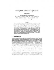
D. Calculation of αk propagation coefficients To calculate of the αk forward propagation coefficients the system is simulated in IP but for the quantizer of interest, k, at SN Ri . This quantizer injects a quantization noise power which is controlled by δk as described in [4]. δk has to be big enough to avoid flooring of the BER curve. As shown in Figure 2, the noise of the quantizer k degrades performance from P1 up to the BER of P2. SN Rq can now be derived out of a pre-computed BER curve of the IP system. Then, αk can be computed as αk = 22δk (10
−SN Rq 10
− 10
−SN Ri 10
)
(7)
Interestingly, by considering rounding quantization, the number of estimations needed becomes a linear function of the number of quantizers, L. Moreover, the impact of the decision-making errors due to quantization is estimated based on Equation 6 and a pre-computed BER curve of the IP system. This two properties make the proposed approach scalable for complex systems. In the case of truncation, the number of estimations needed grows quadratically with L since the quantization noise power mean term is not zero. E. Constraint for quantization degradation In wireless communications, the signal to noise implementation loss is a common metric to characterize the degradation due to the non-idealities of real implementations. The latter specifies the increase in SNR required by the real implementation to deliver the same performance as the ideal receiver. Accordingly, we define the fixed-point degradation, Δ, as the difference in the SNR required by the IP and the FP system to provide a certain performance. � � � � (8) Δ = SN Ri � −4 − SN Rq � −4 10
10
In this work a BER of 10−4 is considered. Notice that this is system dependent and needs to be carefully dimensioned for the different applications. Figure 2 plots the BER curve of both the IP and FP version of a receiver. At SN Ri , an IP receiver would work in P1. However, due to the quantization noise, the actual performance is the one of P2, with an equivalent SNR
QAM-64 BER curve.
of SN Rq . Thus, the FP receiver working point is P3. Δ is the difference in SNR between P2 and P3. IV. E XPERIMENTS A. Case Study 1: FFT in a QAM-64 OFDM receiver FFTs are a key functionality in Orthogonal Frequency Division Multiplexing (OFDM) -based wireless standards, such as WLAN 802.11 n, Mobile WiMAX, 3GPP LTE, etc. In the transmitter considered in this work, a QAM-64 Mapper translates random bits into constellation symbols which are then operated by a 256-points Inverse Fourier Transform (IFFT). The addition of Additive White Gaussian Noise (AWGN) models the channel noise. The receiver performs the inverse operations, FFT and Demapper, to recover the original transmitted bits. The IP BER curve of such OFDM receiver is plotted in Figure 3. A FP 256-points radix-2 FFT is implemented. The latter is constituted by 8 butterfly stages of 128 radix-2 butterflies each. For illustration purposes, a single quantizer, Qk , is inserted at the output of every butterfly belonging to the butterfly stage k. Despite the FFT in isolation is a linear-time-invariant system, in the receiver chain it is followed by non-linear operations. These are affected by the quantization noise of a FP FFT. The slicer operators involved in the Demapper block are a clear example. A slicer is a decision-making operator with an unsmooth region at the exact threshold. Due to the additive channel noise, the input of this slicer has a non-zero probability of sitting in its unsmooth region. In this case, the smallest quantization noise introduced in the FFT can provoke a decision-making error. A.2-3 are violated and perturbation theory fails on predicting the impact of finite precision processing on the final wireless receiver performance. The FP system is simulated with 28 dB SN Ri and the effect of different decimal bit-widths, δ, on different quantizer is exposed. By using Equation 6, the equivalent SN Rq is calculated. Figure 3 shows the working points of the receiver depending on the bit-widths applied in the quantizers. Interestingly, those working points perfectly match the IP BER curve. Therefore the validity of the forward propagation model of Figure 1b is substantiated.
+
y s R
+ -
1/x
s
Fig. 4.
x
+ -
+
y
|x|2
TABLE I M INIMUM δ FOR THE QAM-16 1/2 AND QAM-64 2/3 MODES
x
R
+
+ -
s
x
R
1/b
+ -
s
x
R b
+
y
+ +
+
PED
SSFE data-flow graph.
B. Case Study 2: SSFE near-ML MIMO detector In most recent standards the drastic increase in throughput comes at the expense of complex MIMO detectors. Although linear detectors are mostly implemented so far, its performance significantly degrades with the growth of the modulation scheme. Thus, many implementations of near-ML detectors have recently been published. Concretely, the SSFE (Selective Spanning with Fast Enumeration) [9] is a nearML MIMO detector designed to provide a deterministic and regular data-flow, which enables efficient mappings on parallel programmable architectures. Figure 4 show the data-flow graph of the SSFE algorithm. The signals to be quantized are rounded in black. The SSFE algorithm considered can be configured to evaluate a varying number of constellation symbols around the first estimate for the different antennas. Accordingly, SSFE [1 1 2 4] evaluates 1 constellation symbol at the first antenna, 1 at the second, 2 at the third and 4 at the last one, ordered from stronger to weaker. The group of constellation symbols that are selected to be evaluated depends on the sliced initial estimate. Quantization noise can clearly modify this initial estimate, conditioning also the subsequent selection of constellation symbols. Unlike the propose method, perturbation theory fails on capturing such effects derived from the injected quantization noise. Two 3GPP-LTE modulation modes, namely the 4 antennas SDM (Spatial Division Multiplexing) modulated with QAM16 1/2 and QAM-64 2/3, are quantized. Table 1 shows the minimum bit-widths of the signals quantized for the two modulation modes. Besides, 3 different SSFE modes, namely the [1 1 1 1], [1 1 2 4] and [1 2 4 8] are considered. All the quantizations are constraint by two different Δ: 0.1 and 1 dBs. Notice that the different modulation and SSFE modes reach a BER of 10−4 at different SN Ri , ranging from 18 to 37 dBs. Interestingly, the propose method makes explicit variations on the minimum bit-widths depending on the different options. For the different modulation modes, maximum variations of 2 bits are observed. For the different SSFE modes maximum variations of 1 bit are observed. Finally for the different accuracy constraints, variations up to 2 bits are observed. Importantly, wider variations, up to 4 bits, are observed across the different implementation options. Implementations on reconfigurable architectures, such as FPGA or SWP (Sub-Word Parallel) DSPs [7], can take advantage of these variations in minimum bit-widths to reduce average energy consumption and execution time.
SSFE mode SNR @ BER=10−4 Δ signal y R 1 dB b 1/b PED y R 0.1 dB b 1/b PED
[1 1 1 1] 23 / 37
[1 1 2 4] 19 / 31
[1 2 4 8] 18 / 28
5/6 6/8 5/6 2/2 -/7/8 8 / 10 6/7 3/4 -/-
4/6 6/8 5/6 2/3 3/4 6/7 8 / 10 7/8 3/4 5/6
4/5 6/8 5/6 2/3 3/4 6/7 8 / 10 7/7 3/4 5/6
V. C ONCLUSIONS A new method to evaluate the final impact of finite precision processing in wireless applications is proposed. The latter combines analytical analysis with simulations and extends previous work to include the effect of decision-making errors resulting from quantization. The method can be used for effective dimensioning of minimum bit-widths of wireless DSP algorithm implementations under a given accuracy constraint. Finally, the method described in this paper has a wider ambit than wireless applications. The latter can be applied to any application domain, such as audio and vision, where only signal integrity needs to be kept and approximations can be accommodated without affecting the application performance. R EFERENCES [1] S. Kim, K. Kum, and S. Wonyong, “Fixed-point optimization utility for c and c++ based digital signal processing programs,” IEEE Trans. on Circuits and Systems II, vol. 45, no. 11, pp. 1455–1464, November 1998. [2] A. Oppenheim and R. Schafer, Digital Signal Processing. Englewood Cliffs, NJ: Prentice-Hall, Inc., 1975. [3] P. W. Wong, “Quantization and roundoff noises in fixed-point fir digital filters,” IEEE Trans. on Signal Processing, vol. 39, no. 7, pp. 1552–1563, 1991. [4] B. Widrow, I. Kollar, and M. Liu, “Statistical theory of quantization,” IEEE Trans. on Instrumentation and Measurement, vol. 45, no. 6, pp. 353–61, 1995. [5] L. B. Jackson, Digital filters and signal processing: with MATLAB exercises, 3rd ed. Boston: Kluwer Academic Publishers, 1996. [6] S. Changchun and R. Brodersen, “A perturbation theory on statistical quantization effects in fixed-point dsp with non-stationary inputs,” in Proceedings of the 2004 International Symposium on Circuits and Systems, New Jersey, USA, 2004, pp. 373–376. [7] D. Novo, B. Bougard, A. Lambrechts, L. van der Perre, and F. Cattoor, “Scenario-based fixed-point data format refinement to enable energyscalable software defined radios,” in DATE ’08: Proceedings of the conference on Design, automation and test in Europe. IEEE Press, 2008. [8] R. Rocher, D. Menard, N. Herve, and O. Sentieys, “Fixed-point configurable hardware components,” EURASIP Journal on Embedded Systems, Special issue on Signal Processing with High Complexity: Prototyping and Industrial Design, vol. 2006, pp. 1–13, 2006. [9] M. Li, B. Bougard, W. Xu, D. Novo, L. van der Perre, and F. Cattoor, “The optimization of near-ml mimo detector for parallel programmable architecture,” in DATE ’08: Proceedings of the conference on Design, automation and test in Europe. IEEE Press, 2008.