Finite Queueing Modeling and Optimization: A Selected Review

Hindawi Publishing Corporation Journal of Applied Mathematics Volume 2014, Article ID 374962, 11 pages http://dx.doi.org/10.1155/2014/374962

Research Article Finite Queueing Modeling and Optimization: A Selected Review F. R. B. Cruz1 and T. van Woensel2 1 2

Departamento de Estat´ıstica, Universidade Federal de Minas Gerais, 31270-901 Belo Horizonte, MG, Brazil Department of Industrial Engineering & Innovation Sciences, Eindhoven University of Technology, P.O. Box 513, 5600 MB, Eindhoven, The Netherlands

Correspondence should be addressed to F. R. B. Cruz; [email protected] Received 6 December 2013; Accepted 30 January 2014; Published 23 March 2014 Academic Editor: Nachamada Blamah Copyright © 2014 F. R. B. Cruz and T. van Woensel. This is an open access article distributed under the Creative Commons Attribution License, which permits unrestricted use, distribution, and reproduction in any medium, provided the original work is properly cited. This review provides an overview of the queueing modeling issues and the related performance evaluation and optimization approaches framed in a joined manufacturing and product engineering. Such networks are represented as queueing networks. The performance of the queueing networks is evaluated using an advanced queueing network analyzer: the generalized expansion method. Secondly, different model approaches are described and optimized with regard to the key parameters in the network (e.g., buffer and server sizes, service rates, and so on).

1. Introduction Queueing theory is the mathematical study of waiting lines and it enables the mathematical analysis of several related processes, including arrivals at the queue, waiting in the queue, and being served by the server. The theory enables the derivation and calculation of several performance measures which can be used to evaluate the performance of the queueing system under study. More specifically, the focus in this paper is on finite buffer queueing networks which are characterized by the blocking effect, which eventually degrades the performance, commonly measured via, for example, the throughput of the network. Queueing modeling and optimization of large scale manufacturing systems and complex production lines have been and continue to be the focus of numerous studies for decades (e.g., see Smith [1–3]). Queueing networks are commonly used to model such complex systems (see Suri [4]). The main reason to use queueing modeling is because of their ability to accurately model the resource allocation problems we are interested in (i.e., the buffer, server, and bufferserver combination problems), under approximate Poisson arrivals and general service rates. Of course, there are other methodologies tailored for different settings as, for instance, simulation methods (see Law and Kelton [5]) and advanced methods that explore the spectral characteristics of the

associated matrices in Markovian models (e.g., see the works of Yeralan and Tan [6] and Fadiloglu and Yeralan [7], among others). This review aims at providing an overview of modeling, performance evaluation, and optimization approaches from a queueing theory point of view. Additionally, the algorithms selected were implemented and tested in some basic queueing network topologies, namely, series, merges, and splits. The numerical results provide new insight into this important class of manufacturing network design problems. The paper is structured as follows. In Section 2, we present the performance evaluation method considered for the queueing networks analyzed. Also in Section 2, we elaborate on the different optimization models that exist and discuss some of the optimization tools that are used to optimize these models. Section 3 gives computational results for some selected optimization models for a complex network. Finally, Section 4 concludes the paper and gives some pointers for future research in the area.

2. Material and Methods 2.1. Finite Queueing Networks. Queueing networks are defined as either open, closed, or mixed. In open queueing networks, customers enter the system from outside, receive some service at one or more nodes, and then leave the system.

2 In closed queueing networks, customers never leave or enter the system but a fixed number of customers circulate within the network (see Whitt [9] and Smith [10]). Mixed queueing networks are systems that are open with respect to some customers and are closed with respect to other customers (see Balsamo et al. [11]). Research in the area of queueing networks is very active as we shall see and resulted in a vast amount of journal papers, books, and reports. For a more general discussion on queueing networks, the reader is referred to Walrand [12] among others. In this paper, we will focus on finite queueing networks. The assumption is that the capacity of the buffer space between two consecutive connected service stations is finite. As a consequence, each node in the network might be affected by events at other nodes, leading to the phenomena of blocking or starvation. In the literature, two general blocking mechanisms are presented: blocking after service (BAS) and blocking before service (BBS). BAS occurs when after service a customer sees that the buffer in front of her/him is full and as a consequence s/he cannot continue her/his way in the network. BBS implied that a server can start processing a next customer only if there is a space available in the downstream buffer. If not, the customer has to wait until a space becomes available. Most production lines operate under BAS system. Moreover, in the literature it is the most commonly made assumption regarding the buffer behavior (see Dallery and Gershwin [13]). 2.2. Network Performance Evaluation. Performance evaluation tools for queues include product form methods, numerical methods, approximate methods, and simulation. Let us discuss each of them a bit more in detail. More in-depth information can be found in the references mentioned as follows. Initially, the product form methods decompose the system into single pairs or triplets of nodes instead of analyzing the entire system at once. Details may be found in Perros [14]. Each decomposed node can then be treated as an independent service provider, for which all results and insights of the single node queueing models can be used (see, e.g., Gross et al. [15]). Jackson [16, 17] firstly showed that the joint distribution of the entire network is made up of the product of the marginal distributions at each of the nodes under some strict conditions (e.g., exponential arrivals and services, under no blocking). A decomposition technique yields exact results for queueing networks with product form solutions. For networks without a product form solution, the technique gives a good approximation (see Balsamo et al. [11]). The numerical methods are also useful, as in theory these methods can be used to solve every Markovian model. The problem, however, with numerical solutions is that the state space of queueing networks grows exponentially with the number of nodes, the number of customers, and the number of buffers. As a consequence, numerical methods consume extensive computer time to get to the solution. Numerical methods are applied to smaller networks though (e.g., see Balsamo et al. [11]). Among the approximate methods, the decomposition methods are very popular. These methods are approximate because the subnetworks are only a part of the whole line

Journal of Applied Mathematics and, as such, do not have exactly the same behavior (see Dallery and Gershwin [13]). However, if obtaining an exact solution is too expensive in terms of computational effort, approximate methods are justified. The main challenge with approximate methods is to be as close as possible to the exact values. The accuracy of an approximate method can be tested with numerical solutions (for smaller networks) or by using simulation. The main idea of the decomposition methods is to try to generalize the ideas of independence and product form solutions from the Jackson networks to more general systems. Reiser and Kobayashi [18] and Kuehn [19] were the first to develop this approach. After them, several researchers came up with a similar approach (e.g., Buzacott and Shanthikumar [20] and Alves et al. [21]). Finally, simulation is another way to obtain all relevant performance measures for a queueing network (see Law and Kelton [5]). Successful results on simulation based methods were reported by Cruz et al. [22, 23], Pereira et al. [24], Dorda and Teichmann [25], and Cardoso et al. [26], among many others. 2.3. The Generalized Expansion Method. In this paper, the Generalized Expansion Method (GEM) is used as the prime performance evaluation tool. Consequently, this paper provides a selected review based on the GEM and does not explicitly consider other methodologies to obtain the performance measures. Note that the models described fit any performance evaluation tool. In general, we evaluate the performance of the network via its throughput 𝜃. This throughput (and all other measures, e.g., blocking probability, sojourn time, work-in-process, etc.) can be obtained via a queueing network representation. This queueing network representation then needs to be “solved” to obtain the performance of the given network. Notice that we will focus here on 𝑀/𝐺/𝑐/𝐾 queueing models, which in Kendall notation means a queueing system with Markovian arrival rates, generally distributed service times, 𝑐 servers in parallel in the queue, and a total capacity of 𝐾 users in the queue (including those under service). As it will be detailed soon, the GEM transforms the queueing network into an equivalent Jackson network, which can be decomposed so that each node can be solved independently of each other (similar to a product form solution approach). The GEM is an effective and robust approximation technique to measure the performance of open finite queueing networks. The effectiveness of GEM as a performance evaluation tool has been presented in many papers, including Kerbache and Smith [27–29], Jain and Smith [30], Smith [31], and Andriansyah et al. [32]. The GEM uses BAS, which is prevalent in most systems including production and manufacturing (see Dallery and Gershwin [13]), transportation (see van Woensel and Vandaele [33, 34]), and other similar systems. Developed by Kerbache and Smith [27], the GEM has become an appealing approximation technique for performance evaluation of queueing networks due to its accuracy and relative simplicity. Moreover, exact solutions to performance measurement are restricted only to very simple networks and simulation requires a considerable amount of computational effort.

Journal of Applied Mathematics The GEM is basically a combination of two approximation methods, namely, the repeated trials and the node-bynode decomposition. In order to evaluate the performance of a queueing network, the method first divides the network into single nodes with revised service and arrival parameters. Blocked customers are registered into an artificial “holding node” and are repeatedly sent to this node until they are serviced. The addition of the holding node expands the network and transforms the network into an equivalent Jackson network in which each node can be solved independently. In the remaining part of this section, we will present a high-level overview of the method. For more detailed information and applications of the GEM, the reader is referred to, for example, Kerbache and Smith [28]. The GEM described below assumes that one wants to solve 𝑀/𝐺/𝑐/𝐾 queueing networks. Note that the methodology is generic such that 𝑀/𝑀/1/𝐾, 𝑀/𝑀/𝑐/𝐾, 𝑀/𝐺/1/𝐾, 𝐺𝐼/𝐺/1/𝐾, and 𝐺𝐼/𝐺/𝑐/𝐾 queueing networks could also be analyzed. Only the relevant equations (e.g., the blocking probabilities) need to be adapted for these other cases. There are three main steps in the GEM, namely, network reconfiguration, parameter estimation, and feedback elimination. The notation for the GEM, presented in Basic Network Notation section will be used throughout the paper. The steps are described as follows. Stage I: Network Reconfiguration. For each finite node in the queueing network, an artificial node is created to register the blocked jobs. By introducing such artificial nodes, we also create new routing probabilities in the network. The result of network reconfiguration can be seen from Figure 1. There are two possible states of the finite node, namely, the saturated and the unsaturated states. Arriving jobs will try to access the finite node 𝑗. With a probability of (1 − 𝑝𝐾𝑗 ), the job will find the the finite node unsaturated, when it will enter the queue and eventually be serviced. However, if the finite node 𝑗 is saturated (with a probability of 𝑝𝐾𝑗 ), then the job will be directed to the artificial holding node ℎ𝑗 , where it will be delayed. The delay at the artificial node is modeled using a 𝑀/𝐺/∞ queue, representing a delay time without queueing. Afterward, the blocked job will try to reenter the finite queue 󸀠 ). There is a probability with a success probability of (1 − 𝑝𝐾 𝑗 󸀠 that the blocked job still finds the finite node saturated of 𝑝𝐾 𝑗 and thus it will be directed again to the artificial holding node ℎ𝑗 . This process repeats until the blocked job is able to enter the finite node.

Stage II: Parameter Estimation. At this stage, the values for 󸀠 , and 𝜇ℎ are determined. Notice that the parameters 𝑝𝐾 , 𝑝𝐾 node index 𝑗 is omitted for the sake of simplicity. 𝑝𝐾 : In order to determine 𝑝𝐾 , exact analytical formulas should be used whenever possible (see Kerbache and Smith [29]). For cases where exact 𝑝𝐾 formula is unavailable, approximations for 𝑝𝐾 in 𝑀/𝐺/𝑐/𝐾 setting provided by Smith [31] can be used. These approximations are based on a closed-form expression derivable from the finite capacity exponential queue (𝑀/𝑀/𝑐/𝐾) using Kimura’s [35]

3 M/G/cj /Kj

M/G/ci /Kj

j

i

M/G/ci /Ki

M/G/

pK𝑗

i

(1 −

hj

M/G/cj/Kj ) j

(1 − pK𝑗 )

Figure 1: The generalized expansion method.

two-moment approximation. The following 𝑝𝐾 formula for 𝑀/𝐺/2/𝐾 is presented as an example (see Smith [31]): 𝑝𝐾 =

2

2

2

2

2𝜌2((√𝜌/𝑒𝑠 −√𝜌/𝑒+𝐾)/(2+√𝜌/𝑒𝑠 −√𝜌/𝑒)) (2𝜇 − 𝜆) −2𝜌2((√𝜌/𝑒𝑠 −√𝜌/𝑒+𝐾)/(2+√𝜌/𝑒𝑠 −√𝜌/𝑒)) 𝜆 + 2𝜇 + 𝜆

.

(1)

The 𝑝𝐾 for the 𝑀/𝐺/𝑐/𝐾, for 𝑐 = 3, 4, . . ., will not be shown for brevity but are available in Smith [31]. 󸀠 󸀠 , since no exact method is available to calculate 𝑝𝐾 , 𝑝𝐾 an approximation from Labetoulle and Pujolle [36], based on diffusion techniques, is used: 󸀠 𝑝𝐾

=[

𝜇𝑗 + 𝜇ℎ 𝜇ℎ

−

𝜆 [(𝑟2𝐾 − 𝑟1𝐾 ) − (𝑟2𝐾−1 − 𝑟1𝐾−1 )] 𝜇ℎ [(𝑟2𝐾+1 − 𝑟1𝐾+1 ) − (𝑟2𝐾 − 𝑟1𝐾 )]

−1

] , (2)

in which 𝑟1 and 𝑟2 are the roots of the polynomial. Consider 𝜆 − (𝜆 + 𝜇ℎ + 𝜇𝑗 ) 𝑥 + 𝜇ℎ 𝑥2 = 0,

(3)

󸀠 in which 𝜆 = 𝜆 𝑗 − 𝜆 ℎ (1 − 𝑝𝐾 ), and 𝜆 𝑗 and 𝜆 ℎ are the actual arrival rates to the finite and artificial holding notes, respectively. Furthermore, it can be argued that

̃ (1 − 𝑝 ) = 𝜆 ̃ −𝜆 . 𝜆𝑗 = 𝜆 𝑖 𝐾 𝑖 ℎ

(4)

𝜇ℎ , the delay distribution at the holding node ℎ, is actually nothing but the remaining service time of the finite node 𝑗. Based on the renewal theory, one can formulate the remaining service time distribution as the following rate 𝜇ℎ : 𝜇ℎ =

2𝜇𝑗 1 + 𝜎𝑗2 𝜇𝑗2

,

(5)

in which 𝜎𝑗2 is the service time variance of the finite node 𝑗. At this point, one should notice that if the service time of the finite node is exponentially distributed with rate 𝜇𝑗 , then the memoryless property of exponential distribution will hold, such that 𝜇ℎ = 𝜇𝑗 .

(6)

Stage III: Feedback Elimination. As a result of the feedback loop at the holding node, a strong dependency on the arrival

4

Journal of Applied Mathematics

process is created. In order to eliminate such dependency, the service rate at the holding node must be adjusted as follows: 󸀠 ) 𝜇ℎ . 𝜇ℎ󸀠 = (1 − 𝑝𝐾

(7)

As a consequence, the service rate at node 𝑖 preceding the finite node 𝑗 is affected as well. One can see that the mean service time at node 𝑖 is 𝜇𝑖−1 when the finite node is −1 unsaturated, and 𝜇𝑖−1 + 𝜇ℎ󸀠 when the finite node is saturated. Thus, on average, the mean service time of node 𝑖 preceding the finite node 𝑗 is −1

𝜇𝑖−1 = 𝜇𝑖−1 + 𝑝𝐾 𝜇ℎ󸀠 .

(8)

The above equations apply to all finite nodes in the queueing network. Summary. To sum up, all performance measures of the network can be obtained by solving the following equations simultaneously: 󸀠 ), 𝜆 = 𝜆 𝑗 − 𝜆 ℎ (1 − 𝑝𝐾

̃ (1 − 𝑝 ) , 𝜆𝑗 = 𝜆 𝑖 𝐾 ̃ −𝜆 , 𝜆𝑗 = 𝜆 𝑖 ℎ ̃ −𝜆 , 𝜆𝑗 = 𝜆 𝑖 ℎ 󸀠 𝑝𝐾

=[

𝜇𝑗 + 𝜇ℎ 𝜇ℎ

−

𝜆 [(𝑟2𝐾 − 𝑟1𝐾 ) − (𝑟2𝐾−1 − 𝑟1𝐾−1 )] 𝜇ℎ [(𝑟2𝐾+1 − 𝑟1𝐾+1 ) − (𝑟2𝐾 − 𝑟1𝐾 )]

−1

] , (9)

2

𝑧 = (𝜆 + 2𝜇ℎ ) − 4𝜆𝜇ℎ , 𝑟1 = 𝑟2 =

[(𝜆 + 2𝜇ℎ ) − 𝑧1/2 ] 2𝜇ℎ [(𝜆 + 2𝜇ℎ ) + 𝑧1/2 ] 2𝜇ℎ

𝑝𝐾 ≡ Equation (1) .

, , (10)

Note that (1), for 𝑝𝐾 , only applies to an 𝑀/𝐺/2/𝐾 setting. Other expressions for 𝑝𝐾 for 𝑀/𝐺/𝑐/𝐾 queues, with 𝑐 = 3 to 𝑐 = 10, have been developed by Smith [31] and can be used in the set of (9) and (1). 2.4. Optimization Models. In this section, we review some of the optimization models found in the literature. Given a directed graph 𝐺(𝑉, 𝐴) to represent the queueing network, characterized by Poisson arrivals, in which 𝑉 is the set of node (queues), with nonnegative buffers, multiple servers, and a general service time distribution, and in which 𝐴 is the set of directed arcs (pairs of queues) interconnecting the nodes, we can optimize (i) on the number of buffers, (ii) on the number of servers used in each vertex 𝑉𝑖 , (iii) on the characteristics of the service distribution (e.g., the service rates and/or the service variability), (iv) on the routing probabilities related

to the arcs 𝐴, or (v) on any combination of these possible decision variables. In general, we can write the generic optimization model as follows: 𝑍 = min 𝑓 (x) ,

(11)

subject to Θ (x) ≥ Θ𝜏 , x ≥ 0,

(12)

which minimizes the total allocation 𝑓(x) = ∑𝑖∈𝑉 𝑥𝑖 (i.e., over all vertices 𝑖 ∈ 𝑉), constrained to provide a minimum throughput of Θ𝜏 . A number of specific models can be specified based on the above generic model. (i) When we set x ≡ B, the buffer allocation problem (BAP) appears. One extra constraint needs to be added to reflect the integrality condition, 𝐵𝑖 ∈ N, for all 𝑖 ∈ 𝑉. The objective function is then 𝑍BAP = min ∑𝑖∈𝑉 𝐵𝑖 . This is a model formulation presented and discussed in detail in Smith [37], Smith and Cruz [8], and Smith et al. [38] in which series, merge, and split topologies were examined using the GEM to estimate the performance of these queueing networks and an iterative search methodology based on Powell’s [39] algorithm to find the optimal buffer allocation within the network. The papers of Gershwin and Schor [40] and Shi and Gershwin [41] also deal with buffer allocation. (ii) The server allocation problem (CAP) appears if we have x ≡ c. Again, an extra integrality constraint is needed, 𝑐𝑖 ∈ N, for all 𝑖 ∈ 𝑉. The objective function is then 𝑍CAP = min ∑𝑖∈𝑉 𝑐𝑖 . The CAP was considered by Smith et al. [42] in which a methodology was developed built upon two-moment approximations to the service time distribution embedded in the GEM for computing the performance measures in complex finite queueing networks and Powell’s [39] algorithm for optimally allocating servers to the network topology. (iii) Combining the server and buffer allocation problems by setting x ≡ (B, c) results in the joint buffer and server allocation problem (BCAP). In this case, the integrality constraints are 𝐵𝑖 , 𝑐𝑖 ∈ N, for all 𝑖 ∈ 𝑉. Next to this integrality constraint, one more constraint is needed. It is necessary to ensure that the traffic intensity is such thar 𝜌𝑖 ≡ 𝜆 𝑖 /(𝑐𝑖 𝜇𝑖 ) < 1 to ensure a finite optimal solution. Note that buffers can be equal to zero, hence, having a zero-buffer system (more on bufferless systems in Andriansyah et al. [32] in which such networks were evaluate in terms of the throughput using the GEM that was compared to simulations and a multiobjective optimization approach was adopted to derive the Pareto efficient curves showing the trade-off between the total number of servers used and the throughput). Secondly, note that

Journal of Applied Mathematics

5

the objective function needs to be adapted slightly to take into account the two objectives (i.e., buffers and servers). We consider two options to rewrite the objective function depending on how to deal with the multiobjective issue. (a) First, the objective function can be written as a weighted sum of the two objectives; that is, 𝑍BCAP1 = min {𝜔∑ 𝑐𝑖 + (1 − 𝜔) ∑ 𝐵𝑖 } . 𝑖∈𝑉

(13)

𝑖∈𝑉

We assign a cost of 𝜔 to servers and (1 − 𝜔) to buffers. We can then modify the value of 𝜔, such that 0 < 𝜔 < 1, to reflect the relative cost of servers versus buffers. As 𝜔 is decreased, the cost of servers will become relatively lower than that of buffers. That is, buffers are then more expensive than servers. Alternatively, when the value of 𝜔 is increased, the servers become more costly relative to the buffers. In this way, we evaluate whether different pricing of servers and buffers results in a significantly different buffer and server allocation. It is worthwhile to mention that if 𝜔 = 0, the above problem reduces to the pure BAP and if 𝜔 = 1, the pure CAP is obtained. The BCAP1 problem was treated in details by Woensel et al. [43], when the joint optimization of the number of buffers and servers was firstly solved by means of Powell’s [39] method, a classical nonlinear derivative-free optimization algorithm, while a two-moment approximation and the GEM compute the performance measure of interest (the throughput). The proposed methodology was capable of handling the trade-off between the number of servers and buffers, yielding better throughput than previously published studies. Also, the importance of the squared coefficient of variation of the service time was stressed, since it strongly influenced the approximate optimal allocation. (b) Secondly, the objective function can be formulated in a multicriteria way; that is, 𝑍BCAP2 = min {𝑓1 (c) , 𝑓2 (B)} ,

(14)

in which each one of the two objectives are considered explicitly, with 𝑓1 (c) ≡ ∑𝑖∈𝑉 𝑐𝑖 , and 𝑓2 (B) ≡ ∑𝑖∈𝑉 𝐵𝑖 . Consequently, one obtains an approximation of the Pareto set of solutions for the two objectives. As such, this perspective is more general than the BCAP1 formulation. For further details on multiobjective optimization in general, see Chankong and Haimes [44]. The BCAP2 formulation was treated by Cruz et al. [45, 46] which

developed a multiobjective genetic algorithm to satisfy these conflicting objectives and to produce an approximation of the complete set of all best solutions, known as the Pareto optimal or noninferior set. (iv) A slightly different formulation is the optimal routing problem (OROP). Here, the routing probabilities 𝛼𝑖,𝑗 are determined such that the throughput is maximized. Of course, the sum of all routing probabilities 𝛼𝑖,𝑗 in the arcs leaving each vertex 𝑖 ∈ 𝑉 and reaching its successors 𝑗, such that (𝑖, 𝑗) ∈ 𝐴 should sum up to one 𝑍ORAP = max Θ (𝛼) ,

(15)

subject to 0 ≤ 𝛼𝑖,𝑗 ≤ 1,

∀ (𝑖, 𝑗) ∈ 𝐴,

∑ 𝛼𝑖,𝑗 = 1,

∀𝑖 ∈ 𝑉,

(16)

∀𝑗∈𝛿(𝑖)

in which Θ(𝛼) is the throughput, which is the objective that must be maximized, 𝛼 the optimal routing probability matrix, 𝛼 ≡ [𝛼𝑖,𝑗 ], that is, the matrix that maximizes the objective function of this predefined network, and 𝛿(𝑖) is the set of succeeding vertexes of vertex 𝑖; that is, 𝛿(𝑖) ≡ {𝑗 | (𝑖, 𝑗) ∈ 𝐴}. The throughput will thus be affected by the effective routing of jobs through the network, the variability of the service distribution, the number of servers, and the number of buffers. Among the papers that dealt with the ORAP, we could mention Gosavi and Smith [47] and Daskalaki and Smith [48]. Additionally, Cruz and van Woensel [49] solved the ORAP by using the GEM as the performance evaluation tool of the finite queueing network and optimizing by means of a heuristics based on Powell’s [39] algorithm. (v) A last variation considered is the profit maximization model. The models are thus expanded with financial indicators in order to maximize the profit generated. This profit will be a function of the quantity one can set in the market (i.e., the throughput) and the costs to realize this throughput, which could be the buffer and/or server allocation. The decision variable is thus the investment in buffers or servers ((B, c)). Assume the cost of the buffers or servers is 𝛾 and the gain of a unit of throughput is equal to 𝜙. Then we can formulate the objective function as follows: 𝑍PROFIT = max {𝜙Θ (B, c) − 𝛾∑ (𝐵𝑖 + 𝑐𝑖 ) 𝑖∈𝑉

𝜏

−𝛽 [Θ − Θ (B, c)] } ,

(17)

6

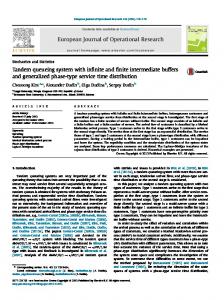
Journal of Applied Mathematics Considering the BCAP model, it can be shown that for a network with 𝑁 nodes, the complexity involved is

5

ZPROFIT

4

[

3

1

0.2

0.4

0.6

X

0

0.8

10

8

6

4

2

Y

(a) 𝑍PROFIT versus 𝑋 ≡ 𝛾/𝜙 and 𝑌 ≡ 𝛽/𝜙

10

1.5

2

1

3.5

2.5

3.5

4

3

4

4.5

9 8 7 6

1.5

2

2.5

3

5

4.5

Y

1

4 3 2

0.5

1.5

0.4

2

0.3 X

2.5

0.2

3

0.1

3.5

4

4.5

1

(18)

Clearly, the solution space grows exponentially in the number of nodes, but not (exponentially) in the capacity of each node. The complexity of the BCAP model can thus be written as 𝑂(𝐾𝑁).

2

0 0

𝐾 (𝐾 + 1) 𝑁 ] . 2

0.6

(b) contour plot

Figure 2: Achieved profit at the optimal buffer allocation for Θ𝜏 = 5.

in which [Θ𝜏 − Θ(B, c)] is either positive or zero (i.e., Θ(B, c) ≤ Θ𝜏 ). Penalty costs of size 𝛽 are charged when the system throughput does not meet the market demand (i.e., Θ(B, c) < Θ𝜏 ). Penalty costs can include the cost of outsourcing production to another factory. Figure 2 displays the behavior of this optimization function for a network of three 𝑀/𝐺/𝑐/𝐾 queues in tandem, with 𝜇𝑖 = 10, 𝑠𝑖2 = 1.5, for all 𝑖, an external arrival rate Λ 1 = 5 and Θ𝜏 = 5. It shows the achieved profit, 𝑍PROFIT , at the optimal buffer allocation, for 𝜙 = 1 and different cost settings 𝛾 and 𝛽. When the operational expense increases (𝑋 ≡ 𝛾/𝜙), it is more attractive to underachieve market demand (i.e., Θ(B, c) ≪ Θ𝜏 ); optimal throughput decreases. When the penalty costs increase (𝑌 ≡ 𝛽/𝜙), it becomes less attractive to underachieve market demand; optimal throughput increases. It is worthwhile to state that the models described above are difficult nonlinear integer programming problems.

2.5. Optimization Methodologies. While the GEM computes the performance measures for the queueing network, many of the above discussed models need to be optimized on the decision variables defined in x. Note that there, of course, exist many optimization methods. An exhaustive discussion is left out of this paper, but the interested reader is referred to Aarts and Lenstra [50] and the references therein. We describe two methodologies which have proven to be successful for the above described models, namely, the Powell’s [39] algorithm and a genetic algorithm approach. Of course, small problems can always be enumerated. Powell’s [39] algorithm can be described as an unconstrained optimization procedure that does not require the calculation of first derivatives of the function. Numerical examples from Himmelblau [51] have shown that the method is capable of minimizing a function with up to twenty variables Powell’s method locates the minimum of 𝑓(x) of a nonlinear function by successive unidimensional searches from an initial starting point x(0) along a set of conjugate directions. These conjugate directions are generated within the procedure itself. Powell’s method is based on the idea that if a minimum of a nonlinear function 𝑓(x) is found along 𝑝 conjugate directions in a stage of the search, and an appropriate step is made in each direction, the overall step from the beginning to the 𝑝-th step is conjugate to all of the 𝑝 subdirections of the search. Genetic algorithms (GA) are optimization algorithms to perform an approximate global search relaying on the information obtained from the evaluation of several points in the search space and obtaining a population of these points that converges to the optimum through the application of the genetic operators mutation, crossover, selection, and elitism. Each of these operators may be implemented in several different ways, each one of them characterizing a specific instance of GA. Additionally, convergence of GA is guaranteed by assigning fitness to each population member and preserving diversity at the same front. For instance, recent successful applications of GA were reported by Lin [52] and Calvete et al. [53], for single-objective applications, and by Carrano et al. [54] and Cruz et al. [45, 46], for multipleobjective applications. A wealth of references is given by these authors. For an application of GA to manufacturing problems, see Andriansyah et al. [32].

3. Results and Insights In this section, we will focus on one example network and describe the results for some of the different optimization

Journal of Applied Mathematics

7

Table 1: Results for the buffer allocation problem (see Smith and Cruz [8]). 2

𝑠 0.5 1.0 1.5

c (1 1 1 1 1 1 1 1 1 1 1 1 1 1 1 1) (1 1 1 1 1 1 1 1 1 1 1 1 1 1 1 1) (1 1 1 1 1 1 1 1 1 1 1 1 1 1 1 1)

2 𝜇 = 10 Λ

B (8 4 4 4 4 4 4 4 4 4 4 4 4 4 4 5) (10 5 5 5 5 4 4 4 4 4 4 4 4 5 5 5) (11 5 5 5 5 5 5 5 5 5 5 5 5 5 5 6)

4 𝜇 = 10

#1

1

𝜇=5

7 𝜇=5

11 𝜇=5

8

12

𝜇=5

𝜇=5

9 𝜇=5

13 𝜇=5

#2 3 𝜇 = 10

5 𝜇 = 10

#1

∑𝑖 𝐵𝑖 69 77 87

𝜃(c, B) 4.9899 4.9879 4.9877

10

6 𝜇=5

#2

#1 𝜇 = 10

∑𝑖 𝑐𝑖 16 16 16

#2

14 𝜇 = 10 16

Θ

𝜇 = 20 15 𝜇 = 10

Figure 3: Combined topology.

models discussed above. We consider a combination of the three basic topologies (series, split, and merge), as shown in Figure 3. This network consists of 16 nodes with the processing rate of servers in each node given in the figure. The network is adopted from Smith and Cruz [8]. We use exactly the same values for Λ, 𝜇, 𝑠2 , and the routing probabilities for the splitting node (#1 and #2). Note that the routing probability #1 refers to the up tier of the node, while #2 refers to the low tier. Refer to Figure 3 for the position of each node in the network. 3.1. The Buffer Allocation Problem (BAP). We reproduce in Table 1 the results from Smith and Cruz [8] for this network structure with Λ = 5 and the routing probabilities equal to 0.5 (Table 29 in their paper). The optimization method used was Powell with multiple restarts to avoid local optima. Note that Smith and Cruz [8] considered an 𝑀/𝐺/1/𝐾 setting and therefore the number of servers in all nodes is set to 1 while optimizing on the buffer allocation. Based on Table 1, we see that the first node (most congested) is receiving more buffers to cope with the relatively high arrival rate. 3.2. The Server Allocation Problem (CAP). Let us now fix the number of buffers beforehand and then optimize on the number of servers used. More specifically, we set all buffers equal to 1 and look at the resulting server allocation. The results are given in Table 2, also obtained from Powell algorithm with multiple restarts to avoid local optima. Interestingly, we observe the same behavior as for the buffer allocation; that is, the first node is receiving more resources than the remaining nodes. On the other hand, the number of servers added is relatively low compared to the buffers added (e.g., 5 versus 8, for 𝑠2 = 0.5). This is because a server is also acting as a buffer, but a server adds more value, measured in throughput, as servers actually provide service.

3.3. The Joint Buffer-Server Allocation Problem (BCAP). Before going to the results for the example network, we analyze the difference between buffers and servers. We saw that the BAP and CAP give different results in terms of number of servers versus number of buffers used. Let us assume that we have a single zero-buffer node with one server (i.e., 𝐾 = 1, 𝐵 = 0, and 𝑐 = 1), submitted to an external arrival rate Λ = 5.0, service rate 𝜇 = 10 and a squared coefficient of variation of the service time distribution 𝑠2 = {0.5, 1.0, 1.5}. Figure 4 gives the percentage increase of adding either a server (adding one to nine servers compared to the base case) or a buffer (adding one to eleven buffers compared to the base case) to the zero buffer base situation. It is clear that in this case, the first added buffer or first added server gives the largest contribution to the throughput value, which is limited by the external arrival rate Λ. Note that the addition of the first extra server gives an increase in throughput of about 58% to 78%, depending upon the squared coefficient of variation of the service time distribution 𝑠2 , while the first added buffer only gives a 36% to 39% increase. Important to mention is that, in order to achieve the same increase in throughput by only using buffers, we need four to six extra buffer spaces, depending on the 𝑠2 , rather than only one server space. The results for the joint buffer-server allocation problem are presented in Table 3, in which the 𝑐/𝐵 price ratio gives an indication of the relative costs of servers compared to buffers, obtained from Powell. A price ratio of 8 : 1, for example, means that servers are 8 times more expensive than buffers. The results from Table 3 show a higher throughput than for the pure BAP, Table 1, for every setting. As expected, we found that the optimal server allocation in the BCAP is different from the server settings in the pure BAP. This, however, depends strongly upon the price ratio of buffers versus servers. We found that 𝑀/𝐺/1/𝐾 is not an optimal

8

Journal of Applied Mathematics Table 2: Results for the server allocation problem. 2

𝑠 0.5 1.0 1.5

c (5 2 2 2 2 2 2 2 2 2 2 2 2 2 2 2) (5 2 2 2 2 2 2 2 2 2 2 2 2 2 2 2) (5 2 2 2 2 2 2 2 2 2 2 2 2 2 2 2)

B (1 1 1 1 1 1 1 1 1 1 1 1 1 1 1 1) (1 1 1 1 1 1 1 1 1 1 1 1 1 1 1 1) (1 1 1 1 1 1 1 1 1 1 1 1 1 1 1 1)

∑𝑖 𝑐𝑖 34 36 34

∑𝑖 𝐵𝑖 16 16 16

𝜃(c, B) 4.9997 4.9996 4.9996

𝑍𝛼 35.29 35.33 35.37

Table 3: Results for the joint buffer-server allocation problem. Λ 5.0

2

𝑠 0.5

𝑐/𝐵 1:8 1:4 1:2 1:1 2:1 4:1 8:1

c (3 3 3 3 3 3 3 3 3 3 3 3 3 3 3 3) (3 3 3 3 3 3 3 3 3 3 3 3 3 3 3 3) (3 3 3 3 3 3 3 3 3 3 3 3 3 3 3 3) (5 3 3 3 3 2 2 2 2 2 2 2 2 3 3 5) (2 2 2 2 2 2 2 2 2 2 2 2 2 2 2 2) (3 1 1 1 1 1 1 1 1 1 1 1 1 1 1 3) (1 1 1 1 1 1 1 1 1 1 1 1 1 1 1 1)

K (3 3 3 3 3 3 3 3 3 3 3 3 3 3 3 3) (3 3 3 3 3 3 3 3 3 3 3 3 3 3 3 3) (3 3 3 3 3 3 3 3 3 3 3 3 3 3 3 3) (5 3 3 3 3 2 2 2 2 2 2 2 2 3 3 5) (5 3 3 3 3 2 2 2 2 2 2 2 2 3 3 5) (3 5 5 5 5 3 3 3 3 3 3 3 3 5 5 3) (11 6 6 6 6 4 4 4 4 4 4 4 4 6 6 11)

∑𝑖 𝑐𝑖 48 48 48 44 32 20 16

∑𝑖 𝐾𝑖 48 48 48 44 44 60 90

∑𝑖 𝐵𝑖 0 0 0 0 12 40 74

𝜃(c, B) 4.9996 4.9996 4.9996 4.9998 4.9989 4.9974 4.9994

𝑍𝛼 5.76 10.0 16.4 22.2 26.5 26.6 23.0

1.0

1:8 1:4 1:2 1:1 2:1 4:1 8:1 1:8 1:4 1:2 1:1 2:1 4:1 8:1

(3 3 3 3 3 3 3 3 3 3 3 3 3 3 3 3) (5 3 3 3 3 2 2 2 2 2 2 2 2 3 3 5) (5 3 3 3 3 2 2 2 2 2 2 2 2 3 3 5) (5 3 3 3 3 2 2 2 2 2 2 2 2 3 3 5) (3 2 2 2 2 2 2 2 2 2 2 2 2 2 2 3) (2 2 2 2 2 1 1 1 1 1 1 1 1 2 2 3) (1 1 1 1 1 1 1 1 1 1 1 1 1 1 1 1) (5 3 3 3 3 2 2 2 2 2 2 2 2 3 3 5) (5 3 3 3 3 2 2 2 2 2 2 2 2 3 3 5) (5 3 3 3 3 2 2 2 2 2 2 2 2 3 3 5) (5 3 3 3 3 2 2 2 2 2 2 2 2 3 3 5) (3 2 2 2 2 2 2 2 2 2 2 2 2 2 2 3) (2 2 2 2 2 1 1 1 1 1 1 1 1 2 2 3) (1 1 1 1 1 1 1 1 1 1 1 1 1 1 1 1)

(3 3 3 3 3 3 3 3 3 3 3 3 3 3 3 3) (5 3 3 3 3 2 2 2 2 2 2 2 2 3 3 5) (5 3 3 3 3 2 2 2 2 2 2 2 2 3 3 5) (5 3 3 3 3 2 2 2 2 2 2 2 2 3 3 5) (3 3 3 3 3 2 2 2 2 2 2 2 2 3 3 3) (6 3 3 3 3 4 4 4 4 4 4 4 4 3 3 4) (13 6 6 6 6 4 4 4 4 4 4 4 4 6 6 13) (5 3 3 3 3 2 2 2 2 2 2 2 2 3 3 5) (5 3 3 3 3 2 2 2 2 2 2 2 2 3 3 5) (5 3 3 3 3 2 2 2 2 2 2 2 2 3 3 5) (5 3 3 3 3 2 2 2 2 2 2 2 2 3 3 5) (3 3 3 3 3 2 2 2 2 2 2 2 2 3 3 3) (6 3 3 3 3 4 4 4 4 4 4 4 4 3 3 4) (15 7 7 7 7 4 4 4 4 4 4 4 4 7 7 15)

48 44 44 44 34 25 16 44 44 44 44 34 25 16

48 44 44 44 40 60 94 44 44 44 44 40 60 104

0 0 0 0 6 35 78 0 0 0 0 6 35 88

4.9994 4.9997 4.9997 4.9997 4.9984 4.9989 4.9987 4.9996 4.9996 4.9996 4.9996 4.9979 4.9983 4.9986

5.94 9.09 15.0 22.3 26.2 28.1 24.1 5.24 9.15 15.0 22.4 26.8 28.7 25.4

1.5

configuration for this particular queueing network structure, except when buffers are becoming relatively too expensive. For these cases, we found that single-servers are optimal indeed (see rows where 𝑐/𝐵 ratio is 8 : 1). We observe that (near) zero-buffer configurations are identified where appropriate; that is, where the servers are relatively cheaper compared to buffers. Varying the squared coefficient of variation of the service time distribution 𝑠2 does result in some changes in the optimal server and buffer allocation, which shows the importance of models dealing with general service times. The results show that the number of buffers seems to be large under high variability, which could be expected since the increase in 𝑠2 means an increase in the variability. The extra buffers are there to handle this high variability. 3.4. Final Remarks and Insights. The above numerical results for the buffer allocation problem, the server allocation problem, and the joint buffer-server allocation problem show that significant gains can be achieved in manufacturing systems. Specifically, setting the buffers and servers in an appropriate way greatly affects the throughput for these manufacturing systems. This is important as these systems need to be as

highly utilized as possible, given the high investments. Our models and optimizations show that the optimal configurations are not always straightforward and thus advanced models and solution methods are needed. We have followed a queueing network approach with finite buffers, as this resembles reality the closest. This modeling approach is of course much harder than, for example, infinite queueing networks. We see based on the various experiments that our solution methodology is powerful and suitable for the different types of models handled in this paper. This offers managers and manufacturing systems designers a powerful tool to work with. We saw that the BAP and CAP obviously give different results. We also note that while the addition of the first extra server gives a certain amount of increase in the throughput, the addition of the first buffer space generally will give a lower increase. In other words, in order to achieve the same increase in throughput by only using buffers, we need more extra buffer spaces rather than only a few server space.

4. Conclusions This review provided an overview of the different modeling issues, the performance evaluation, and optimization

Journal of Applied Mathematics

9

Change in (%)

0.8 0.6 0.4 0.2 0.0 0

2

4

6

8

c s2 = 1.5 s2 = 1.0 s2 = 0.5

(a) percentual increase in 𝜃 versus Δ𝑐

Change in (%)

0.8 0.6 0.4

behavior of the models based on cycle time, work-in-process (WIP), or other performance measures. In a number of industrial improvement projects carried out, we observed that the critical issue to be able to use the above models is related to data availability. More specifically, processing rates, arrival rates, uncertainty in the service process, and so on need to be extracted from the available databases. An interesting approach to obtaining the relevant data is the effective process time (EPT) point of view (see Hopp and Spearman [55]). The advantage of the effective process time (EPT) approach is that various types of disturbances on the shop-floor are aggregated into EPT distributions, this enables effective modeling. However, it is important to note that, disturbances which are aggregated into the EPT distribution cannot be analyzed afterwards. Hence, shopfloor realities or disturbances which are modeled explicitly and excluded from aggregation in the EPT are defined beforehand. Topics for future research on the queueing part include the analysis and optimization of networks with cycles, for example, to model many important industrial systems that have loops, such as systems with captive pallets and fixtures or reverse streams of products due to rework, or even the extension to GI/G/c/K queueing networks with generally distributed and independent arrivals.

Basic Network Notation

0.2 0.0 0

2

4

6

8

10

B s2 = 1.5 s2 = 1.0 s2 = 0.5

(b) percentual increase in 𝜃 versus Δ𝐵

Figure 4: Throughput increase versus added number of servers (Δ𝑐) and buffers (Δ𝐵).

approaches of the manufacturing systems assuming a queueing theory approach. We discussed the merits of the Generalized Expansion Method as a performance evaluation tool of the finite queueing networks. This methodology has proved in the literature to be a valuable approach. Secondly, different optimization models are discussed, namely the buffer allocation problem, the server allocation problem, the joint buffer, server allocation problem, and some other models. The different optimization models are shown to be hard nonlinear integer programming problems which are able to be approximately solved with a Powell heuristic. The paper ended with an overview of some results for the different models considered on a complex queueing network. 4.1. Future Research Suggestions. In this paper, we considered the throughput as the main performance measure. Instead of the throughput, it would be interesting to evaluate the

Λ: 𝜆𝑗: ̃ : 𝜆 𝑗 𝜇𝑗 :

External Poisson arrival rate to the network Poisson arrival rate to node 𝑗 Effective arrival rate to node 𝑗 Exponential mean service rate at finite node 𝑗 Effective service rate at finite node 𝑗 due to 𝜇̃𝑗 : blocking Blocking probability of finite queue 𝑗 of 𝑝𝐾𝑗 : size 𝐾𝑗 󸀠 𝑝𝐾 : Feedback blocking probability in the 𝑗 expansion method The artificial holding node (queue) ℎ𝑗 : preceding node 𝑗 created in the GEM Number of servers at node 𝑗 𝑐𝑗 : Total capacity at node 𝑗 including the items 𝐾𝑗 : in service 𝐵𝑗 ≡ 𝐾𝑗 − 𝑐𝑗 : Buffer capacity at node 𝑗 excluding the items in service 𝑁: Set of nodes (queues) in the queueing network 𝑉: Set of arcs (pairs of nodes) in the queueing network 𝜌𝑗 ≡ 𝜆 𝑗 /(𝑐𝑗 𝜇𝑗 ): Traffic intensity at node 𝑗 Mean throughput rate at node 𝑗 𝜃𝑗 : Squared coefficient of variation of the 𝑠𝑗2 : service time distribution at node 𝑗.

Conflict of Interests The authors declare that there is no conflict of interests regarding the publication of this paper.

10

Acknowledgments The research of professor Frederico Cruz has been partially funded by the Brazilian agencies, CNPq (Conselho Nacional de Desenvolvimento Cient´ıfico e Tecnol´ogico) of the Ministry for Science and Technology of Brazil, CAPES (Coordenac¸a˜ o de Aperfeic¸oamento de Pessoal de N´ıvel Superior), and FAPEMIG (Fundac¸a˜ o de Amparo a` Pesquisa do Estado de Minas Gerais).

References [1] J. M. Smith, “𝑀/𝐺/𝑐/𝐾 performance models in manufacturing and service systems,” Asia-Pacific Journal of Operational Research, vol. 25, no. 4, pp. 531–561, 2008. [2] J. M. Smith, “Properties and performance modelling of finite buffer 𝑀/𝐺/1/𝐾 networks,” Computers & Operations Research, vol. 38, no. 4, pp. 740–754, 2011. [3] J. M. Smith, “M/G/c/K performance models in manufacturing and service systems,” International Journal of Production Research, 2013. [4] R. Suri, “An overview of evaluative models for flexible manufacturing systems,” Annals of Operations Research, vol. 3, no. 1, pp. 13–21, 1985. [5] A. M. Law and W. D. Kelton, Simulation Modeling and Analysis, McGraw-Hill, New York, NY, USA, 3rd edition, 1982. [6] S. Yeralan and B. Tan, “Analysis of multistation production systems with limited buffer capacity—I. The subsystem model,” Mathematical and Computer Modelling, vol. 25, no. 7, pp. 109– 122, 1997. [7] M. M. Fadiloglu and S. Yeralan, “General theory on spectral properties of state-homogeneous finite-state quasi-birth-death processes,” European Journal of Operational Research, vol. 128, no. 2, pp. 402–417, 2001. [8] J. M. Smith and F. R. B. Cruz, “The buffer allocation problem for general finite buffer queueing networks,” IIE Transactions, vol. 37, no. 4, pp. 343–365, 2005. [9] W. Whitt, “Open and closed models for networks of queues,” AT&T Bell Laboratories Technical Journal, vol. 63, no. 9, pp. 1911– 1979, 1984. [10] J. M. Smith, “Optimal workload allocation in closed queueing networks with state dependent queues,” Annals of Operations Research, 2013. [11] S. Balsamo, V. de Nitto Person´e, and R. Onvural, Analysis of Queueing Networks with Blocking, Kluwer Academic Publishers, Dordrecht, The Netherlands, 2001. [12] J. Walrand, An Introduction to Queueing Networks, PrenticeHall, Englewoord Cliffs, NJ, USA, 1988. [13] Y. Dallery and S. B. Gershwin, “Manufacturing flow line systems: a review of models and analytical results,” Queueing Systems, vol. 12, no. 1-2, pp. 3–94, 1992. [14] H. G. Perros, “Queueing networks with blocking: a bibliography,” ACM Sigmetrics, vol. 12, pp. 8–12, 1984. [15] D. Gross, J. F. Shortle, J. M. Thompson, and C. M. Harris, Fundamentals of Queueing Theory, Wiley-Interscience, Hoboken, NJ, USA, 4th edition, 2008. [16] J. R. Jackson, “Networks of waiting lines,” Operations Research, vol. 5, pp. 518–521, 1957. [17] J. R. Jackson, “Jobshop-like queueing systems,” Management Science, vol. 10, no. 1, pp. 131–142, 1963.

Journal of Applied Mathematics [18] M. Reiser and H. Kobayashi, “Accuracy of the diffusion approximation for some queuing systems,” Journal of Research and Development, vol. 18, pp. 110–124, 1974. [19] P. J. Kuehn, “Approximate analysis of general queuing networks by decomposition,” IEEE Transactions on Communications, vol. 27, no. 1, pp. 113–126, 1979. [20] J. A. Buzacott and J. G. Shanthikumar, Stochastic Models of Manufacturing Systems, Prentice-Hall, Englewood Cliffs, NJ, USA, 1993. [21] F. S. Q. Alves, H. C. Yehia, L. A. C. Pedrosa, F. R. B. Cruz, and L. Kerbache, “Upper bounds on performance measures of heterogeneous 𝑀/𝑀/𝑐 queues,” Mathematical Problems in Engineering, vol. 2011, Article ID 702834, 18 pages, 2011. [22] F. R. B. Cruz, J. M. Smith, and R. O. Medeiros, “An M/G/c/C state-dependent network simulation model,” Computers and Operations Research, vol. 32, no. 4, pp. 919–941, 2005. [23] F. R. B. Cruz, P. C. Oliveira, and L. Duczmal, “State-dependent stochastic mobility model in mobile communication networks,” Simulation Modelling Practice and Theory, vol. 18, no. 3, pp. 348– 365, 2010. [24] L. A. Pereira, L. H. Duczmal, and F. R. B. Cruz, “Congested emergency evacuation of a population using a finite automata approach,” Safety Science, vol. 51, no. 1, pp. 267–272, 2013. [25] M. Dorda and D. Teichmann, “Modelling of freight trains classification using queueing system subject to breakdowns,” Mathematical Problems in Engineering, vol. 2013, Article ID 307652, 11 pages, 2013. [26] R. T. N. Cardoso, R. H. C. Takahashi, and F. R. B. Cruz, “Pareto optimal solutions for stochastic dynamic programming problems via Monte Carlo simulation,” Journal of Applied Mathematics, vol. 2013, Article ID 801734, 9 pages, 2013. [27] L. Kerbache and J. M. Smith, “The generalized expansion method for open finite queueing networks,” European Journal of Operational Research, vol. 32, no. 3, pp. 448–461, 1987. [28] L. Kerbache and J. M. Smith, “Asymptotic behavior of the expansion method for open finite queueing networks,” Computers and Operations Research, vol. 15, no. 2, pp. 157–169, 1988. [29] L. Kerbache and J. M. Smith, “Multi-objective routing within large scale facilities using open finite queueing networks,” European Journal of Operational Research, vol. 121, no. 1, pp. 105– 123, 2000. [30] S. Jain and J. M. Smith, “Open finite queueing networks with M/M/C/K parallel servers,” Computers and Operations Research, vol. 21, no. 3, pp. 297–317, 1994. [31] J. M. Smith, “M/G/c/K blocking probability models and system performance,” Performance Evaluation, vol. 52, no. 4, pp. 237– 267, 2003. [32] R. Andriansyah, T. van Woensel, F. R. B. Cruz, and L. Duczmal, “Performance optimization of open zero-buffer multi-server queueing networks,” Computers & Operations Research, vol. 37, no. 8, pp. 1472–1487, 2010. [33] T. van Woensel and N. Vandaele, “Empirical validation of a queueing approach to uninterrupted traffic flows,” 4OR, vol. 4, no. 1, pp. 59–72, 2006. [34] T. van Woensel and N. Vandaele, “Modeling traffic flows with queueing models: a review,” Asia-Pacific Journal of Operational Research, vol. 24, no. 4, pp. 435–461, 2007. [35] T. Kimura, “A transform-free approximation for the finite capacity M/G/s queue,” Operations Research, vol. 44, no. 6, pp. 984–988, 1996.

Journal of Applied Mathematics [36] J. Labetoulle and G. Pujolle, “Isolation method in a network of queues,” IEEE Transactions on Software Engineering, vol. 6, no. 4, pp. 373–381, 1980. [37] J. M. Smith, “Optimal design and performance modelling of 𝑀/𝐺/1/𝐾 queueing systems,” Mathematical and Computer Modelling, vol. 39, no. 9-10, pp. 1049–1081, 2004. [38] J. M. Smith, F. R. B. Cruz, and T. van Woensel, “Topological network design of general, finite, multi-server queueing networks,” European Journal of Operational Research, vol. 201, no. 2, pp. 427–441, 2010. [39] M. J. D. Powell, “An efficient method for finding the minimum of a function of several variables without calculating derivatives,” The Computer Journal, vol. 7, pp. 155–162, 1964. [40] S. B. Gershwin and J. E. Schor, “Efficient algorithms for buffer space allocation,” Annals of Operations Research, vol. 93, pp. 117– 144, 2000. [41] C. Shi and S. B. Gershwin, “An efficient buffer design algorithm for production line profit maximization,” International Journal of Production Economics, vol. 122, no. 2, pp. 725–740, 2009. [42] J. M. Smith, F. R. B. Cruz, and T. van Woensel, “Optimal server allocation in general, finite, multi-server queueing networks,” Applied Stochastic Models in Business and Industry, vol. 26, no. 6, pp. 705–736, 2010. [43] T. van Woensel, R. Andriansyah, F. R. B. Cruz, J. M. Smith, and L. Kerbache, “Buffer and server allocation in general multi-server queueing networks,” International Transactions in Operational Research, vol. 17, no. 2, pp. 257–286, 2010. [44] V. Chankong and Y. Y. Haimes, Multiobjective Decision Making: Theory and Methodology, vol. 8, North-Holland, New York, NY, USA, 1983. [45] F. R. B. Cruz, T. Van Woensel, and J. M. Smith, “Buffer and throughput trade-offs in M/G/1/K queueing networks: a bicriteria approach,” International Journal of Production Economics, vol. 125, no. 2, pp. 224–234, 2010. [46] F. R. B. Cruz, G. Kendall, L. While, A. R. Duarte, and N. L. C. Brito, “Throughput maximization of queueing networks with simultaneous minimization of service rates and buffers,” Mathematical Problems in Engineering, vol. 2012, Article ID 692593, 19 pages, 2012. [47] H. D. Gosavi and J. M. Smith, “An algorithm for sub-optimal routeing in series-parallel queueing networks,” International Journal of Production Research, vol. 35, no. 5, pp. 1413–1430, 1997. [48] S. Daskalaki and J. M. Smith, “Combining routing and buffer allocation problems in series-parallel queueing networks,” Annals of Operations Research, vol. 125, pp. 47–68, 2004. [49] F. R. B. Cruz and T. van Woensel, “Optimal routing in general finite multi-server queueing networks,” under review, 2014. [50] E. Aarts and J. K. Lenstra, Local Search in Combinatorial Optimization, Princeton University Press, Princeton, NJ, USA, 2nd edition, 2003. [51] D. M. Himmelblau, Applied Nonlinear Programming, McGrawHill, New York, NY, USA, 1972. [52] F.-T. Lin, “Solving the knapsack problem with imprecise weight coefficients using genetic algorithms,” European Journal of Operational Research, vol. 185, no. 1, pp. 133–145, 2008. [53] H. I. Calvete, C. Gal´e, and P. M. Mateo, “A new approach for solving linear bilevel problems using genetic algorithms,” European Journal of Operational Research, vol. 188, no. 1, pp. 14– 28, 2008. [54] E. G. Carrano, L. A. E. Soares, R. H. C. Takahashi, R. R. Saldanha, and O. M. Neto, “Electric distribution network multiobjective design using a problem-specific genetic algorithm,”

11 IEEE Transactions on Power Delivery, vol. 21, no. 2, pp. 995– 1005, 2006. [55] W. J. Hopp and M. L. Spearman, Factory Physics, Waveland Press, Long Grove, Ill, USA, 3 edition, 2011.

Advances in

Operations Research Hindawi Publishing Corporation http://www.hindawi.com

Volume 2014

Advances in

Decision Sciences Hindawi Publishing Corporation http://www.hindawi.com

Volume 2014

Journal of

Applied Mathematics

Algebra

Hindawi Publishing Corporation http://www.hindawi.com

Hindawi Publishing Corporation http://www.hindawi.com

Volume 2014

Journal of

Probability and Statistics Volume 2014

The Scientific World Journal Hindawi Publishing Corporation http://www.hindawi.com

Hindawi Publishing Corporation http://www.hindawi.com

Volume 2014

International Journal of

Differential Equations Hindawi Publishing Corporation http://www.hindawi.com

Volume 2014

Volume 2014

Submit your manuscripts at http://www.hindawi.com International Journal of

Advances in

Combinatorics Hindawi Publishing Corporation http://www.hindawi.com

Mathematical Physics Hindawi Publishing Corporation http://www.hindawi.com

Volume 2014

Journal of

Complex Analysis Hindawi Publishing Corporation http://www.hindawi.com

Volume 2014

International Journal of Mathematics and Mathematical Sciences

Mathematical Problems in Engineering

Journal of

Mathematics Hindawi Publishing Corporation http://www.hindawi.com

Volume 2014

Hindawi Publishing Corporation http://www.hindawi.com

Volume 2014

Volume 2014

Hindawi Publishing Corporation http://www.hindawi.com

Volume 2014

Discrete Mathematics

Journal of

Volume 2014

Hindawi Publishing Corporation http://www.hindawi.com

Discrete Dynamics in Nature and Society

Journal of

Function Spaces Hindawi Publishing Corporation http://www.hindawi.com

Abstract and Applied Analysis

Volume 2014

Hindawi Publishing Corporation http://www.hindawi.com

Volume 2014

Hindawi Publishing Corporation http://www.hindawi.com

Volume 2014

International Journal of

Journal of

Stochastic Analysis

Optimization

Hindawi Publishing Corporation http://www.hindawi.com

Hindawi Publishing Corporation http://www.hindawi.com

Volume 2014

Volume 2014