Finite-Time Consensus with Disturbance Rejection ... - Semantic Scholar

1

Finite-Time Consensus with Disturbance Rejection by Discontinuous Local Interactions in Directed Graphs Mauro Franceschelli, Member, IEEE, Alessandro Pisano, Member, IEEE, Alessandro Giua, Senior Member, IEEE, Elio Usai, Member, IEEE Abstract—In this paper we propose a decentralized discontinuous interaction rule which allows to achieve consensus in a network of agents modeled by continuous-time first-order integrator dynamics affected by bounded disturbances. The topology of the network is described by a directed graph. The proposed discontinuous interaction rule is capable of rejecting the effects of the disturbances and achieving consensus after a finite transient time. An upper bound to the convergence time is explicitly derived in the paper. Simulation results, referring to a network of coupled Kuramoto-like oscillators, are illustrated to corroborate the theoretical analysis. Index Terms—Multi-agent systems, consensus, discontinuous control, distributed control, disturbance rejection.

I. I NTRODUCTION The consensus problem for networked systems, i.e., the problem of steering the states of a set of agents towards a common value exploiting only local interactions, finds application in several domains ranging from networks of power generators [1], coordination of flocks of mobile autonomous vehicles [2], [3], [4], [5], synchronization of dynamical systems such as clocks or oscillators [6], [7] and others. Linear interaction rules, as those considered in the above works, always lead to the asymptotic achievement of consensus. In [8] the control problem for synchronization of large networks is addressed via pinning control, a method which consists in controlling only a subset of systems possibly small in number to achieve the desired emerging behavior even if many systems are not directly controlled and the graph that describes the network topology of the uncontrolled agents is only weakly connected or possibly a simple directed forest. General nonlinear interaction rules are considered in [9] for multiagent systems modeled in discrete time where also undirected timevarying network topologies and time-varying delays are taken into account. In [10] the authors study the consensus problem for discretetime second order multi-agent systems considering state transition matrices that are stochastic but with possibly negative elements. Several works have recently appeared in the literature that exploit appropriate nonlinear interaction rules to achieve consensus after a transient of finite length (finite-time consensus). More specifically, in [11] the concept of finite time semistability has been developed and applied to solve the finite time consensus problem for networked systems with static network topology and agents modeled as continuous time integrators. In [12], finite time consensus by means of discontinuous protocols based on signed gradient flows has been developed and applied to networks of first order dynamics. In [4] M. Franceschelli, A. Pisano, A. Giua, E. Usai are with the Dept. of Electrical and Electronic Engineering, University of Cagliari, Cagliari, Italy. Email: {mauro.franceschelli,pisano,giua,usai}@diee.unica.it. Alessandro Giua is also with LSIS, University of Aix-Marseille, Marseille, France. The research leading to these results has been partially supported from the European Union Seventh Framework Programme [FP7/2007-2013] under grant agreement n 257462 HYCON2 Network of excellence, Artemis JU (GA number 333020) as part of the project ACCUS, project PGR00152-RObust Decentralised Estimation fOr large-scale systems (RODEO) of the Italian Ministry for Foreign Affairs and by Regione Sardegna LR 7/2007 (call 2010) under project SIAR (CRP-24709).

and [5], hybrid finite-time consensus protocols exploiting a synergic combined use of continuous and discontinuous control algorithms have been proposed with application, respectively, to rendezvous of mobile robots and formation control for agents modeled by single integrators. In [13], finite-time consensus is achieved in the framework of a leader-follower problem. Agents are modeled by second order dynamics and the suggested solution takes the form of a discontinuous local interaction rule. In [14], discontinuous interaction protocols are proposed for finite time formation tracking by making reference to agents governed by single or double integrator dynamics and considering directed network topologies. In [15], finite time consensus is established for first and second order agents with nonlinear dynamics considering a static network topology with an undirected graph. In [16] and [17] the finite time consensus problem is solved in discrete time for single integrator agents with static and directed network topologies. The approach requires each agent to know the minimal polynomial of the iteration matrix that governs the discrete state updates, and the authors propose a decentralized computation scheme for the required parameters. Some works that consider the switching topology case have appeared for undirected or balanced graphs. In [18], the finite-time consensus problem for first order systems is investigated considering a general class of nonlinear local interaction terms, and stability was proved for static and switching undirected graphs. In [19], the finitetime consensus problem is addressed for networks of continuous time integrators by employing an interaction rule consisting, for each agent, of a weighted sum of fractional powers of the differences between the agent state and that of its neighbors. The authors show that finite time consensus is achieved provided that the network topology stays connected for sufficiently long intervals of time. In [20] and [21], finite-time consensus algorithms are provided for networks of unperturbed integrators by exploiting discontinuous local interaction rules under time varying (both undirected and directed) network topologies. In [22], the authors study discontinuous binary protocols for finite time consensus in directed graphs. We also note that the consensus problem with quantized state variables may lead to finite time convergence results as shown in [23] and [24]. All the above works focus on demonstrating the finite time achievement of consensus, and none of them accounts for external disturbances or unknown coupling terms in the network dynamics. The robust consensus problem for a network of agents affected by noise, disturbances, measurements errors or unmodeled perturbations has been addressed in different forms by several authors [25], [26], [27], [28]. In [25], the consensus problem in the presence of measurements errors is studied in the discrete-time setting, with reference to linear consensus protocols with constant or vanishing weights. In [26], a class of non-linear continuous protocols is investigated that achieve the so-called “ϵ-consensus”, namely an approximate agreement condition where the state of all agents converge towards a common set, in spite of the presence of additive disturbances. In [27], the continuous-time consensus problem is studied in the case of quantized information exchange between agents which is a particular kind of discontinuous feedback where the effect of quantization can be seen as a disturbance. In [28], the finite time consensus problem is investigated for networks of agents affected by Gaussian white noise and the associated convergence properties are characterized in a probabilistic setting. The main contribution of the present work, which considers a network of perturbed continuous time integrators along with a directed communication topology, is to provide for the finite time achievement of an exact consensus condition while explicitly accounting for the presence of unknown bounded disturbances affecting the agents’ dynamics. In [29], similarly to the present work, we

2

have considered a network of first-order integrators perturbed by unknown disturbances, by considering a switching but undirected network topology. The proposed solution was only able to provide disturbance attenuation. Here we propose a different protocol that is able to achieve complete disturbance rejection in directed graphs with static topology. Noticeably, the presented analysis makes use of non smooth Lyapunov analysis arguments. The use of a discontinuous control action is necessary to achieve complete disturbance rejection as discussed in [30] in that a standard finite gain controller which depends continuously on state variables, in absence of a model of the disturbance and knowledge of the network topology, is only able to attenuate the effect of the disturbances on the output but not cancel them out if they are time-varying and unknown. This paper is structured as follows. In Section II the problem statement and system model are introduced. In Section III the convergence and robustness properties of the suggested decentralized interaction rule are characterized. In Section IV numerical simulations for a network of Kuramoto-like agents are provided to corroborate the theoretical analysis. In Section V some concluding remarks are given, and the Appendix Section contains some background result on the solution concept for discontinuous dynamical systems. II. P ROBLEM STATEMENT Let us consider n agents connected by a communication network whose topology is described by a directed graph G = (V, E), where V = {1, . . . , n} denotes the set of agents and E ⊆ {V × V } is the set of edges representing communication channels between the agents. The graph contains an edge (i, j) ∈ E directed from agent j to agent i if agent i receives information from agent j. Furthermore, let L = {lij } denote the Laplacian matrix of graph G whose elements are defined as   |Ni | if i = j, −1 if (i, j) ∈ E, lij = (1)  0 otherwise, where Ni ⊆ V denotes the set of neighbors of agent i, i.e., the set of agents that send informations to the i-th agent. The cardinality of Ni is called in-degree of agent i, and it is referred to as δin,i = |Ni |. A directed path p is an ordered sequence of directed edges that connect two nodes in V . A rooted directed spanning tree is a graph which contains no cycles with the property that there exist a node, called root, from which every other node is reachable by walking a directed path. Let x = [x1 , x2 , ..., xn ]T represent the state of the entire network of agents that are modeled by the perturbed first order integrator dynamics x˙ i (t) = νi (x, t) + ui (t),

xi (0) = xi0 ,

∀i ∈ V,

(2)

where νi (x, t) is an unknown term representing couplings, perturbations or disturbances corrupting the i-th agent dynamics, ui (t) is the local control input and xi0 is the initial condition. Due to the explicit dependence of νi (x, t) on the entire state vector x, this representation takes into account the possibility that the dynamics of the agents are affected by the state of other agents also without the availability of a direct communication channel between them. By stacking the input and disturbance variables into the vectors u = [u1 , u2 , ..., un ]T and ν = [ν1 , ν2 , ..., νn ]T one obtains the next compact representation of the network dynamics x(t) ˙ = ν(x, t) + u(t). Denote νˆ(x, t) = ν(x, t) −

1Tn ν(x, t) 1n , n

(3) (4)

where 1n = [1, 1, ..., 1]T ∈ Rn . Vector νˆ(x, t) represents the deviation of the disturbance term ν(x, t) from its time-varying T average value 1 ν(x,t) . In the rest of the paper we make the following n assumption Assumption 1: ν(x, t) is continuous in x and t and there exists a known constant Π ≥ 0 such that ∥ˆ ν (x, t)∥1 =

n ∑

|ˆ νi (x, t)| ≤ Π,

∀x ∈ Rn , ∀t ∈ R+ ,

(5)

i=1

 Our objective is to develop a local interaction rule ui (t) compatible with the current graph topology and guaranteeing, in spite of the presence of disturbances that satisfy Assumption 1, the following finite-time consensus property ∃tr ∈ R+ :

|xi (t) − xj (t)| = 0,

∀t > tr , ∀i, j ∈ V,

(6)

where tr is the finite transient time. The proposed discontinuous control protocol takes the form ( ) ui (t) = −k · sign Li x(t) , (7) where k is the tuning constant of the algorithm, Li is the i-th row of the Laplacian matrix, and sign(·) is the sign function defined as follows  if z > 0  1 0 if z = 0 sign(z) = (8)  −1 if z < 0 It is useful to remark that the discontinuous protocol (7) can be equivalently written as   ∑ ui (t) = −k · sign  (xi (t) − xj (t)) , i ∈ V. (9) j∈Ni

Denote σi (x) = sign(Li x(t)),

i ∈ V,

(10)

and define vector σ(x) = [σ1 , σ2 , ..., σn ]T .

(11)

We can therefore rewrite the control vector in compact form as u(t) = −k · σ(x),

(12)

and the next closed-loop collective agent dynamics arises x(t) ˙ = ν(x, t) − k · σ(x).

(13)

In the following, we intend the solutions to eq. (13) in the sense of Filippov. Solutions are not unique and their existence is guaranteed by the fact that x(t) ˙ exists almost everywhere by definition and its bounded. In the proof of Theorem 3.3 we introduce and adopt the necessary tools of non-smooth Lyapunov analysis to analyse the convergence properties of eq. (13). The next proposition states two relationships that shall be instrumental to prove the main contribution of this paper. Proposition 2.1: Consider the networked dynamics (13) where graph G = (V, E) contains at least a rooted directed spanning tree. If there exists a pair (i, j) ∈ E such that xi ̸= xj , i.e., the network is not at consensus, then the next properties hold: i) Vector σ(x) has at least one element different from zero. ii) σ(x)T Lσ(x) ≥ 1. (14) Proof of i)

3

Consider the sets of maximal and minimal nodes defined as follows: Vmax = {i ∈ V | (∀j ∈ V ) xi ≥ xj ), Vmin = {i ∈ V | (∀j ∈ V ) xi ≤ xj ). Since the network is not at consensus, both sets are not empty and they are disjoint. Obviously, if i ∈ Vmax then σ(xi ) ≥ 0 and in particular σ(xi ) > 0 iff there exists an arc (i, j) such that xj ̸∈ Vmax . Dually, one can see that if i ∈ Vmin then σ(xi ) < 0 iff there exists an arc (i, j) such that xj ̸∈ Vmin . Since graph G contains a rooted directed spanning tree, from the root node there exists a directed path that reaches every other node. At least one these two cases must hold. If the root node does not belong to Vmax , consider a path from the root to a node in Vmax : along this path there must be an arc (i, j) ∈ Vmax × (V \ Vmax ), hence σ(xi ) ̸= 0. If the root node does not belong to Vmin , consider a path from the root to a node in Vmin : along this path there must be an arc (i, j) ∈ Vmin × (V \ Vmin ), hence σ(xi ) ̸= 0 thus proving property i). Proof of property ii) In what follows we omit the dependence of σi (x) from x. The left hand side of (14) can be rewritten as follows σ(x)T Lσ(x) =

n ∑ i=1

σi

∑ j∈Ni

(σi − σj ) =

n ∑ ∑

σi (σi − σj ) ≥ 0.

i=1 j∈Ni

(15) Since σi ∈ {−1, 0, 1} for i = 1, . . . , n we get that the term σi (σi − σj ) can only be either 0, 1 or 2. It was proved in the previous step i) that at least one entry of vector σ(x) is not zero if the network state is not at consensus. Define the disjoint subsets V+1 , V−1 and V0 of V as follows V+1 = {i ∈ V : σi = 1}, V−1 = {i ∈ V : σi = −1}, V0 = {i ∈ V : σi = 0}.

(16)

Obviously, the above sets constitute a partition of V , i.e., V+1 ∪ V−1 ∪ V0 ≡ V

(17)

It readily follows from the previous step i) that the cardinality of either set V+1 or V−1 is at least one if the network is not in the consensus state. On the other hand, since σi (σi − σj ) = 0 ∀i ∈ V0 , one can rewrite (15) as follows ∑ ∑ ∑ ∑ σ(x)T Lσ(x) = σi (σi − σj ) + σi (σi − σj ) . i∈V+1 j∈Ni

i∈V−1 j∈Ni

(18) Since the graph G contains a rooted directed spanning tree, if the network is not at consensus there exists at least a path that connects two nodes that belong to different sets with at least one node not in V0 . It follows that in such a path we can consider the directed arc (i, j) ∈ E with either i ∈ V+1 and j ∈ V0 ∪ V−1 or with i ∈ V−1 and j ∈ V0 ∪ V+1 . If i ∈ V+1 or i ∈ V−1 and j ∈ V0 then σi (σi − σj ) = 1

(19)

On the contrary if i ∈ V−1 and j ∈ V1 (or, analogously, i ∈ V+1 and j ∈ V−1 ) this would imply the next relation σi (σi − σj ) = 2

(20)

By taking the worst case condition (19) one can conclude that at least one term σi (σi − σj ) in the right hand side of (18) is greater than or equal to one and Proposition 2.1 is proven. 

III. C ONVERGENCE ANALYSIS AND MAIN RESULT We now present the formal proof of convergence of the proposed control protocol showing the finite time attainment of the consensus condition for the considered network of agents and the complete rejection of the disturbance terms provided that the control gain k is taken large enough. Let us define the disagreement vector of the state vector as 1n 1Tn x(t), (21) n Clearly, convergence to consensus implies the convergence to the origin of the disagreement vector. We now recall the Clarke’s definition of generalized gradient [31] that will be exploited in our main result. Definition 3.1 (Clarke generalized gradient): Let V : Rn → R be locally Lipschitz continuous and define δ(t) = x(t) −

∂C V (x) , co {limi→∞ ∇V (xi )|xi → x, xi ∈ / ΩV ∪ N } , where co denotes the convex hull, ΩV is the set of Lebesgue measure zero where the gradient ∇V (x) does not exists and N is an arbitrary set of measure zero.  Moreover, we recall the conditions under which the chain rule can be exploited in non-smooth Lyapunov analysis [32]. Proposition 3.2 (Chain rule): If V : Rn → R is locally Lipshitz continuous and x : R → Rn is absolutely continuous, then for almost every t there exists p ∈ ∂C V (x(t)) such that d [V (x(t))] = pT x˙ dt  We are now ready to state the main result of this paper. Theorem 3.3: Consider the collective agents dynamics (13) and let assumption (5) be satisfied. If the considered graph G contains at least a rooted directed spanning tree and the gain parameter k satisfies the inequality k ≥ 2δin,max Π + ϵ,

ϵ > 0,

(22)

where δin,max = maxi∈V δin,i denotes the maximum in-degree of graph G, Π is the bound given in Assumption 1 and ϵ is an arbitrary positive constant, then the consensus condition expressed by eq. (6) is attained within a finite transient time tr such that tr ≤

∥Lδ(0)∥1 . ε

(23)

Proof: Let zi = Li δ(t), where Li denotes the i-th row of matrix L, and z = [z1 , . . . , zn ]T such that z = Lδ(t). Consider the next non-smooth Lyapunov function ∑ d [V (z(t))] = |zi | = ∥z∥1 . dt i=1 n

(24)

For z1 ̸= 0, z2 ̸= 0, . . . , zn ̸= 0 the time derivative of eq. (24) is well defined and it given by V˙ (t) =

n n ∑ ∑ ∂V z˙i = sign(zi )z˙i . ∂zi i=1 i=1

(25)

The reminder of this proof borrows its main idea from [33] (chapt. 3, Theorem 3, pp. 157-158). If any of the variables zi is zero, the definition of V˙ (t) becomes non trivial since the corresponding right hand side becomes discontinuous. Let us define the sets I0 = {i ∈ V : zi = 0} and I̸= = {i ∈ V : zi ̸= 0}. We interpret the corresponding discontinuous differential equation and its solution in the sense of Filippov [33]. We now consider the Clarke generalized

4

gradient of V (z) as in definition 3.1, which in our case since V (z) is the 1-norm of z takes the form ∂C V (z) = pT

∑ ∑ d SIGN (zi )z˙i . [V (z(t))] ∈ sign(zi )z˙i + dt i∈I i∈I

∑

sign(zi )z˙i + T ˙ = σ(δ(t)) Lδ(t).

=

i∈I̸=

∑ i∈I0

sign(zi )z˙i

= x˙ −

1n 1Tn x˙ n

1n 1Tn (ν(x, t) − k · σ(x)) n = νˆ(x, t) − k · σ(x) + γ(t)1n ,

= ν(x, t) − k · σ(x) −

(28)

(29)

(30)

where 1n 1Tn 1T ν(x, t), γ(t) = n k σ(x). (31) n n In light of eqs. (30)-(31), the time derivative (29) can be rewritten νˆ(x, t) = ν(x, t) −

as d dt

[V (z(t))]

= =

σ(x)T L (ˆ ν (x, t) − k · σ(x) + γ(t)1n ) −k · σ(x)T Lσ(x) + σ(x)T Lˆ ν (x, t) +γ(t)σ(x)T L1n .

(32)

By noticing that L1n = 0, one can simplify (32) as d dt

[V (z(t))] (t)

=

(35)

It is well known that ∥L∥∞ = 2δin,max .

|σ(x)T Lˆ ν (x, t)| ≤ 2δin,max Π.

where σ(δ(t)) is defined as in eq. (11). Therefore, the generalized d time derivative dt [V (z(t))] which in general is a set valued function, in our case is a well defined function to which for every t it corresponds a single point in the real line. Note that both in (27) and (29) the term involving the indexes i ∈ I0 is identically zero as a consequence of the fact that z˙i = 0 ∀i ∈ I0 . Rather than removing such term it is more convenient to keep it, as proposed in (chapt. 3, Theorem 3, pp. 157-158) of [33], d [V (z(t))] in a form which is suitable for as it allows to express dt the next analysis. The dynamics of δ(t) are obtained by differentiating (21) and considering (13) and (10), which yields ˙ δ(t)

∥Lˆ ν (x, t)∥1 ≤ ∥L∥∞ ∥ˆ ν (x, t)∥1 .

(36)

Considering (36) and (5) into (35) we finally get

Since we deal with solutions in the sense of Filippov, the case in which zi (t) = 0 holds for isolated time instants of measure zero can be disregarded in those instants of time [33]. As interestingly noticed in (chapt. 3, Theorem 3, pp. 157-158) of [33], if any of the conditions zi (t) = 0 holds along an interval of time of positive measure then, at those time instants, ∀i ∈ I0 z˙i exists in the sense of Filippov and it takes zero value, i.e. z˙i = 0 ∀i ∈ I0 . We can therefore modify the second term in the right hand side of eq. (27), and exploiting the fact that in our particular case zi = 0 implies z˙ = 0 we find that the set d of points from which dt [V (z(t))] defined in eq. (27) takes values consists in a single point corresponding to [V (z(t))]

(34)

The next estimation holds by virtue of the H¨older inequality

(27)

0

where SIGN (·) is the multivalued function  1 if z > 0,  [−1, 1] if z = 0, SIGN (z) ∈  −1 if z < 0.

d dt

∑ i = |∑ n ˆ(x, t)| i=1 σi (x)L ν n i ≤ ∑i=1 |σi (x)L νˆ(x, t)| i ≤ n ˆ(x, t)| = ∥Lˆ ν (x, t)∥1 i=1 |L ν

|σ(x)T Lˆ ν (x, t)|

(26)

where p ∈ Rn is a vector whose elements pi for i = 1, . . . , n are pi = sign(zi ) if i ∈ I̸= or pi ∈ SIGN (zi ) if i ∈ I0 . Since V (z) is locally Lipshitz continuous we can compute the generalized time derivative of V (z(t)) according to Proposition 3.2 as follows

̸=

It holds that

−k · σ(x)T Lσ(x) + σ(x)T Lˆ ν (x, t). (33)

(37)

Therefore, substituting (37) in (33) and taking into account Proposition 2.1 with relation (14), it yields d [V (z(t))] ≤ −k + 2δin,max Π. (38) dt Considering the tuning condition (22) into the right hand side of eq. (38) then one has that d [V (z(t))] ≤ −ε < 0, dt

(39)

for almost all t as long as there exists i ∈ V such that Li δi (t) ̸= 0, i.e., the consensus state has not been reached. Summarizing, it holds V (x) > 0 V (x) = 0

d [V (z(t))] ≤ −ε dt d [V (z(t))] = 0 and dt

and

for x ̸= α1, α ∈ R (40) for x = α1, α ∈ R

(41)

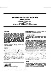
therefore, all solutions converge to the invariant set α1, α ∈ R. From (40), the finite time consensus property with a transient time satisfying (23) is easily verified since ε is a constant lower bound to [ ] d ˙  dt V (t) and Theorem 3.3 is proved. IV. N UMERICAL SIMULATIONS In this section we provide some numerical simulations of the proposed scheme to corroborate the theoretical results. We consider a network of 20 perturbed Kuramoto-like oscillators in which the bounded non-linear couplings, along with additional noise components, are collected into the disturbance term 1∑ νi (x, t) = ωi + sin(xi (t) − xj (t)) + µi (t), (42) n j∈Ni i = 1, 2, ..., n where ωi ∈ [0.1, 0.2] is an input bias, different for each agent and randomly selected, and µi (t) ∈ [0, 0.1] is a random noise with uniform distribution. The network topology is described by a randomly generated directed graph with 20 nodes, shown in Figure 1, which contains a directed spanning tree. By considering the actual topology of the considered example, the worst case bound on the norm of the perturbation deviation vector νˆ(x, t) can be quantified as follows

1T ν(x, t)

≤ 0.4773. ∥ˆ ν (x, t)∥1 = ν(x, t) − 1 (43)

n 1 For the chosen network topology it has been evaluated that δin,max = 3. For the computation of the control gain in accordance with relation (22) we choose ϵ = 0.01, therefore the minimal control gain providing convergence according to (22) is 2δin,max Π + ϵ = 2.85, and the value k = 3 has been adopted in the first test. The continuous time system (13)-(42) has been simulated by using the Euler integration method with a fixed sampling time dt = 10−4 .

5

10 k=6 k=3

V(t)

8 6 4 2 0 0

0.05

0.1

0.15

0.2

0.25

0.3

Time

Fig. 1. Graph representing the directed network topology. (Direction of edges is not shown to improve visual quality)

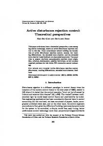
Fig. 4. Finite time transient evolution of the Lyapunov function (24) for k = 3 and k = 6.

V. C ONCLUSIONS AND FUTURE WORK 1

x(t)

0.8 0.6 0.4 0.2 0 0

0.05

0.1

0.15

0.2

0.25

0.3

Time Fig. 2. Transient evolution of the network state x(t) subject to control action with gain k = 3.

In this paper we proposed a decentralized algorithm to solve the finite time consensus problem in a network of integrators affected by bounded disturbances with directed communication topology. A robustness analysis of the proposed discontinuous consensus algorithm, that proves complete disturbance rejection, has been provided. An interesting outcome of the robustness analysis is the link between the maximum in-degree of the underlying network and the minimal amplitude of the control action needed to fully reject the disturbances. Finally, numerical simulations making reference to a network of perturbed Kuramoto-like oscillators have been provided. Future work might be devoted to extend the robustness analysis to networks with switching topology and/or agents governed by more complex dynamics. R EFERENCES

In Figure 2 it is shown the evolution of the network state x(t) in the first test by taking the initial conditions at random within the interval xi (t) ∈ [0, 1]. It is seen that consensus is achieved after a transient of about 0.2s. Figure 3 shows the evolution of the network state x(t) obtained in a second test where the higher value of the control gain k = 6, twice of that used in the first test, was used. Comparing the Figures 2 and 3 shows that increasing the gain speeds up the convergence to consensus. The price to be paid, however, is higher chattering (i.e., high-frequency and small-amplitude vibrations of the state variables) once consensus has been achieved in the discrete-time approximation of the closed loop network dynamics. Figure 4 depicts a comparison between the time evolutions of the Lyapunov function (24) in the two previously outlined tests with different control gain k.

1

x(t)

0.8 0.6 0.4 0.2 0 0

0.05

0.1

0.15

0.2

0.25

0.3

Time Fig. 3. Transient evolution of the network state x(t) subject to control action with gain k = 6.

[1] F. Dorfler and F. Bullo, “Synchronization and transient stability in power networks and non-uniform Kuramoto oscillators,” in American Control Conference, Baltimore, MD, USA, Jun. 2010, pp. 930–937. [2] R. Olfati-Saber, “Flocking for multi-agent dynamic system: Algorithms and theory,” IEEE Trans. on Automatic Control, vol. 51, pp. 401–420, 2006. [3] V. Blondel, J. Hendrickx, A. Olshevsky, and J. Tsitsiklis, “Convergence in multiagent coordination, consensus, and flocking,” in Proc. 44th IEEE Conf. on Decision and Control, Seville, Spain, Dec. 2005, pp. 2996– 3000. [4] Q. Hui, “Finite-time rendezvous algorithms for mobile autonomous agents,” IEEE Transactions on Automatic Control, vol. 56, no. 1, pp. 207 –211, Jan. 2011. [5] F. Xiao, L. Wang, J. Chen, and Y. Gao, “Finite-time formation control for multi-agent systems,” Automatica, vol. 45, no. 11, pp. 2605 – 2611, 2009. [6] L. Schenato and F. Fiorentin, “Average timesynch: a consensus-based protocol for time synchronization in wireless sensor networks,” Automatica, vol. 47, no. 9, pp. 1878–1886, 2011. [7] A. Jadbabaie, N. Motee, and M. Barahona, “On the stability of the kuramoto model of coupled nonlinear oscillators,” in American Control Conference, vol. 5. IEEE, 2004, pp. 4296–4301. [8] W. Yu, G. Chen, J. L¨u, and J. Kurths, “Synchronization via pinning control on general complex networks,” SIAM Journal on Control and Optimization, vol. 51, no. 2, pp. 1395–1416, 2013. [9] Y. Chen, J. Lu, X. Yu, and Z. Lin, “Consensus of discrete-time multiagent systems with transmission nonlinearity,” Automatica, vol. 49, no. 6, pp. 1768 – 1775, 2013. [10] Y. Chen, J. L¨u, X. Yu, and Z. Lin, “Consensus of discrete-time secondorder multiagent systems based on infinite products of general stochastic matrices,” SIAM Journal on Control and Optimization, vol. 51, no. 4, pp. 3274–3301, 2013. [11] Q. Hui, W. M. Haddad, and S. Bhat, “Finite-time semistability and consensus for nonlinear dynamical networks,” IEEE Transactions on Automatic Control, vol. 53, no. 8, pp. 1887–1890, 2008. [12] J. Cort´es, “Finite-time convergent gradient flows with applications to network consensus,” Automatica, vol. 42, no. 11, pp. 1993–2000, 2006.

6

[13] S. Khoo, L. Xie, and Z. Man, “Robust finite-time consensus tracking algorithm for multirobot systems,” IEEE/ASME Transactions on Mechatronics,, vol. 14, no. 2, pp. 219–228, 2009. [14] Y. Cao, W. Ren, and Z. Meng, “Decentralized finite-time sliding mode estimators and their applications in decentralized finite-time formation tracking,” Systems and Control Letters, vol. 59, no. 9, pp. 522 – 529, 2010. [15] Y.Cao and W. Ren, “Finite-time consensus for second-order multi-agent networks with inherent nonlinear dynamics under an undirected fixed graph,” in 50th IEEE Conference on Decision and Control and European Control Conference, Orlando, FL, USA, Dec 2011. [16] S. Sundaram and C. Hadjicostis, “Finite-time distributed consensus in graphs with time-invariant topologies,” in American Control Conference, July 2007, pp. 711 –716. [17] S. Sundaram and C. N. Hadjicostis, “Distributed functional calculation and consensus using linear iterative strategies,” IEEE Journal on Selected Areas in Communications (Special Issue on “Control and Communications”), vol. 26, no. 4, pp. 650 –660, 2008. [18] F. Jiang and L. Wang, “Finite-time information consensus for multiagent systems with fixed and switching topologies,” Physica D, vol. 238, no. 16, pp. 1550–1560, 2009. [19] L. Wang and F. Xiao, “Finite-time consensus problems for networks of dynamic agents,” IEEE Transactions on Automatic Control, vol. 55, no. 4, pp. 950–955, 2010. [20] P. Menon and C. Edwards, “A discontinuous protocol design for finitetime average consensus,” in IEEE Conference on Control Applications, 2010, pp. 2029–2034. [21] S. Rao and D. Ghose, “Sliding mode control-based algorithms for consensus in connected swarms,” International Journal of Control, vol. 84, no. 9, pp. 1477–1490, 2011. [22] G. Chen, F. L. Lewis, and L. Xie, “Finite-time distributed consensus via binary control protocols,” Automatica, vol. 47, no. 9, pp. 1962 – 1968, 2011. [23] F. Ceragioli, C. D. Persis, and P. Frasca, “Discontinuities and hysteresis in quantized average consensus,” Automatica, vol. 47, no. 9, pp. 1916– 1928, 2011. [24] P. Frasca, R. Carli, F. Fagnani, and S. Zampieri, “Average consensus on networks with quantized communication,” International Journal of Robust and Nonlinear Control, vol. 19, pp. 1787 – 1816, 2009. [25] A. Garulli and A. Giannitrapani, “Analysis of consensus protocols with bounded measurement errors,” Systems & Control Letters, vol. 60, no. 1, pp. 44–52, 2011. [26] D. Bauso, L. Giarr´e, and R. Pesenti, “Consensus for networks with unknown but bounded disturbances,” Siam Journal on Control and Optimization, vol. 48, pp. 1756–1770, 2009. [27] P. Frasca, “Continuous-time quantized consensus: Convergence of krasovskii solutions,” Systems & Control Letters, vol. 61, no. 2, pp. 273 – 278, 2012. [28] Y. Zheng, W. Chen, and L. Wang, “Finite-time consensus for stochastic multi-agent systems,” International Journal of Control, vol. 84, no. 10, pp. 1644–1652, 2011. [29] M. Franceschelli, A. Pisano, A. Giua, and E. Usai, “Finite-time consensus based clock synchronization by discontinuous control,” Nonlinear Analysis. Hybrid Systems., vol. 10, no. 1, pp. 83–93, 2013. [30] A. Pisano and E. Usai, “Sliding mode control: A survey with applications in math,” Mathematics and Computers in Simulation, vol. 81, no. 5, pp. 954 – 979, 2011. [31] F. Clarke, Optimization and Nonsmooth Analysis. Wiley-Interscience, New-York, 1983, vol. 18. [32] B. Paden and S. Sastry, “A calculus for computing filippov’s differential inclusion with application to the variable structure control of robot manipulators,” IEEE Transactions on Circuits and Systems,, vol. 34, no. 1, pp. 73 – 82, 1987. [33] A. F. Filippov, Differential Equations with Discontinuous Righthand Sides: Control Systems. Springer, 1988, vol. 18.