Finite Volume Spectrum of 2D Field Theories from Hirota Dynamics

arXiv:0812.5091v2 [hep-th] 5 Dec 2009

AEI-08-NNNN LPTENS-08/68 DESY 08-193

Finite Volume Spectrum of 2D Field Theories from Hirota Dynamics Nikolay Gromovα , Vladimir Kazakovβ and Pedro Vieiraγ

α

DESY Theory, Notkestr. 85 22603 Hamburg Germany; II. Institut f¨ ur Theoretische Physik Universit¨ at Hamburg Luruper Chaussee 149 22761 Hamburg Germany; St.Petersburg INP, Gatchina, 188 300, St.Petersburg, Russia nikgromov AT gmail.com β

Laboratoire de Physique Th´eorique de l’Ecole Normale Sup´erieure et l’Universit´e Paris-VI, 75231, Paris CEDEX-05, France; kazakov AT lpt.ens.fr

γ

Max-Planck-Institut f¨ ur Gravitationphysik, Albert-Einstein-Institut, Am M¨ uhlenberg 1, 14476 Potsdam, Germany; Departamento de F´ısica e Centro de F´ısica do Porto Faculdade de Ciˆencias da Universidade do Porto Rua do Campo Alegre, 687, 4169-007 Porto, Portugal pedrogvieira AT gmail.com

Abstract

We propose, using the example of the O(4) sigma model, a general method for solving integrable two dimensional relativistic sigma models in a finite size periodic box. Our starting point is the so-called Y-system, which is equivalent to the thermodynamic Bethe ansatz equations of Yang and Yang. It is derived from the Zamolodchikov scattering theory in the cross channel, for virtual particles along the non-compact direction of the space-time cylinder. The method is based on the integrable Hirota dynamics that follows from the Y-system. The outcome is a nonlinear integral equation for a single complex function, valid for an arbitrary quantum state and accompanied by the finite size analogue of Bethe equations. It is close in spirit to the Destri-deVega (DdV) equation. We present the numerical data for the energy of various states as a function of the size, and derive the general L¨ uscher-type formulas for the finite size corrections. We also re-derive by our method the DdV equation for the SU (2) chiral Gross-Neveu model.

Contents 1 Introduction and Summary

3

2 TBA and Y-system for O(4) sigma model, or SU (2) Principal Chiral Field

7

2.1

The Model . . . . . . . . . . . . . . . . . . . . . . . . . . . . . . . . . . . . . . . . . . . . . .

7

2.2

TBA and Y-system . . . . . . . . . . . . . . . . . . . . . . . . . . . . . . . . . . . . . . . . . .

8

2.3

Hirota equations . . . . . . . . . . . . . . . . . . . . . . . . . . . . . . . . . . . . . . . . . . .

10

2.4

Asymptotic Bethe Ansatz and Classification of the Solutions . . . . . . . . . . . . . . . . . .

12

2.5

Probing the finite volume . . . . . . . . . . . . . . . . . . . . . . . . . . . . . . . . . . . . . .

13

2.6

Exact solution for the vacuum . . . . . . . . . . . . . . . . . . . . . . . . . . . . . . . . . . . .

14

2.7

Generalization to U (1) sector . . . . . . . . . . . . . . . . . . . . . . . . . . . . . . . . . . . .

15

3 Finite size spectrum for a general state of PCF 3.1

3.2

17

Exact equations for the finite volume spectrum . . . . . . . . . . . . . . . . . . . . . . . . . .

18

3.1.1

Closed equation on the gauge function g(x) . . . . . . . . . . . . . . . . . . . . . . . .

21

3.1.2

Finite size Bethe equations and the energy . . . . . . . . . . . . . . . . . . . . . . . .

22

Large volume limit: ABA and L¨ uscher corrections . . . . . . . . . . . . . . . . . . . . . . . .

23

3.2.1

25

Single particle case . . . . . . . . . . . . . . . . . . . . . . . . . . . . . . . . . . . . . .

4 SU (2) Chiral Gross-Neveu model and related models

26

5 Numerics

28

6

5.1

Implementation of numerics and Mathematica code . . . . . . . . . . . . . . . . . . . . . . . .

29

5.2

Discussion of numerical results . . . . . . . . . . . . . . . . . . . . . . . . . . . . . . . . . . .

31

Conclusions 6.1

33

Summary of the main formulae . . . . . . . . . . . . . . . . . . . . . . . . . . . . . . . . . . .

34

A Derivation of the (ground state) Y -system

35

B General solution in terms of Hirota functions

41

B.1 The main Bethe equations . . . . . . . . . . . . . . . . . . . . . . . . . . . . . . . . . . . . . .

42

C Proof of reality of Tk

43

D Proof of analyticity of T−1 in the physical strip

44

D.1 Analyticity in the U (1) sector . . . . . . . . . . . . . . . . . . . . . . . . . . . . . . . . . . . .

44

D.2 General case . . . . . . . . . . . . . . . . . . . . . . . . . . . . . . . . . . . . . . . . . . . . . .

44

E Details on L¨ uscher formulae derivation

45

2

1

Introduction and Summary

The study of the properties of Quantum Field Theories (QFT’s) in finite volume, or at finite temperature, has a long history and numerous applications. Matsubara description [1] of finite temperature T thermodynamics, by considering the system in the periodic imaginary time t, has lead to the extensive study of the Euclidean QFT’s with one compactified dimension with numerous physical applications [2]. L¨ uscher found the leading finite size corrections to the mass gap in relativistic two dimensional QFT’s [3, 4]. These corrections depend solely on the asymptotic S-matrix of the theory. Recently, L¨ uscher corrections to various multi-particle states in integrable 2D QFT were conjectured [5]. For the integrable 2D QFT’s, as understood during the last two decades, the ambitions can be much higher: these systems are usually solvable at any finite size though a systematic approach to such solutions, as well as a good understanding of the working prescriptions, are still missing. t s

Figure 1: Physical channel, cross-channel and finite volume vs finite temperature. There are two main schemes to address the finite size calculations. The first, pioneered by Destry and deVega (DdV) [6], is based on the integrable discretization. Once such discretization is at hand, the system can be studied by the well established methods based on the transfer matrix approach and the resulting non-linear integral equation (NLIE), often called the DdV equation, calculates not only the ground state energy but also the spectrum of excited states. The method appeared to be very powerful when applied to the Sine-Gordon model [7, 9, 11, 12, 13], or to more general RSOS models [14], Toda theories [15], hard hexagon models [16], etc. However, for generic integrable QFT it is far from easy to find the corresponding integrable lattice regularization and for many models such discretization is not known. Nevertheless, the problem can be usually tackled by using a computation scheme alternative to the DdV approach. As explained in the seminal work of Al.Zamolodchikov [17] this is achieved by the double Wick rotation trick: using the Matsubara imaginary time formulation we can first find the free energy in the infinite volume but finite temperature. Next we flip the meaning of euclidian time and space directions on the cylinder: τ → σ, σ → τ , and interpret the free energy as the ground state of the system in finite volume L = T1 (see fig.1). In this way we can obtain the exact finite volume ground state energy. This computational scheme is known by the name of Thermodynamic Bethe Ansatz (TBA). The TBA equations, whose number is infinite in many interesting models, can be usually concisely casted into the so called Y-system functional equations [18, 19]. Often the latter one can be

3

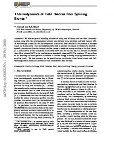
E L/2p

-

L Figure 2: Plots of energies E of a few excited states of O(4) model on a circle of a circumference L L. The vertical axis corresponds to the values of 2π E, the horizontal axis - to the values of L in the logarithmic scale. The lowest curve depicts the vacuum energy. The next one, labeled as θ0 , shows the mass gap energy. The corresponding state is in the U (1) sector, with a single particle at rest, hence with the mode number = 0. The next states in the U (1) sector are denoted by θn1 n2 n3 ,··· , according to the mode numbers n1 , n2 , n3 , . . . excited for the 1-st, 2-nd, 3-rd, etc., particles. For all these states the SU (2)L and SU (2)R spins of the several particles are pointing in the same direction, say they are spin “up”. The dashed line represents a state having a polarization out of the U (1) sector, with left and right “magnons” excited - it corresponds to the quantum state of two particles where both SU (2)L and SU (2)R spins are in the singlet s = 0 state. The qualitative explanation of these graphs will be given in subsection 5.2. rewritten in the form of DdV equations or some similar set of integral equations for a finite set of functions. The method was successfully used for many relativistic models [20, 21, 22, 23, 24]. As explained in the previous paragraph the computation of the exact ground state energy by means of this method is a relatively straightforward task with solid theoretical foundations. To obtain the exact spectrum comprising all excited states of the theory is, on the other hand, a much more involved - and a very interesting - task. A possibility to describe the excited states within the TBA approach, by modifying the analytical properties of the thermodynamic functions, was first suggested in [24]. Another possible way to obtain the spectrum of the theory, proposed around the same time, is based on the analytic continuation of the ground state energy with respect to the parameters of the model, such as the mass or the chemical potential, in order to find the excited states [25]. If the integrable lattice regularization is absent, it is not well understood why these methods work. Nevertheless, the results are usually in the excellent agreement with the perturbation theory, L¨ uscher finite size corrections and the direct Monte-Carlo study for a wide range of sizes L (see for example [26, 27, 28, 29, 30] for O(n) and related σ-models).

4

Lü scher correction Bethe ansatz

Conformal theory

E(L)/m

Hirota dynamics

Thermodynamical Bethe ansatz Lm Figure 3: Domains of applicability of different descriptions of an integrable field theory at a finite volume L. In the ultra-violet regime, for small volume measured in units of a dynamically generated mass, the theory could be described by a conformal theory. In the infrared, at large volume, one can use the asymptotic Bethe equations. The leading order finite size corrections are governed by the (generalized) L¨ uscher corrections. At any volume but for the ground state energy only one can use Thermodynamical Bethe ansatz. Hirota equation, equivalent to Y-system but more efficient when it comes to imposing appropriate analyticity properties, is a universal tool covering the whole diagram. For models with diagonal scattering, like the Sinh-Gordon theory [31], the whole classification of excited states is possible [32]. The situation is much more complex when we deal with the nondiagonal scattering. The nested structure of the corresponding Bethe ansatz equations leads to complicated magnon-type excitations and bound states. Little is known about the excited states in such finite size systems. The only models where the polarized excited states were investigated, using the DdV equations, are the Sine-Gordon model [7] and its supersymmetric version [11] as well as the tricritical Ising model [10]. By the existing methods only the sectors with diagonal scattering can be studied efficiently, as was done for example for the O(4) sigma model in [30]. A general and unified description of all excited states of the σ-models like O(n) or the SU (N ) principal chiral field (PCF), and similar ones, having a “geometric” target space, is still absent. The main goal of the present paper is to give a method of a general and systematic description of all the states of integrable QFT’s in finite volume. We will explain how to go beyond the asymptotic spectrum and compute the full finite size spectrum comprising all excited states of integrable sigma models. We do it here on the example of O(4) sigma model and also for the SU (2) chiral GrossNeveu model but our formalism is certainly more general and is most probably applicable to any integrable 1+1 dimensional σ-models. The main ingredients of the method are: • The two-particles S-matrix for integrable system allows us to write the periodicity condition quantizing the momenta of the physical particles on a large circle of length R. The equations following from the periodicity condition are so called asymptotic Bethe ansatz (ABA) equations describing all states of the model. The details of this computation for the SO(4) sigma

5

model are given in Appendix A1 . They are, however, valid only in a sufficiently big volume compared to the typical interaction distance, Rm ≫ 1 where m is the infinite volume mass gap. • For the ground state, the double Wick rotation (σ, τ ) → (τ, σ) allows to reduce the problem to the thermodynamics. One can put the euclidian theory on the torus with one radius, R, very large and another one, L, arbitrary (see the fig.1). The ground state energy for a finite radius is related to the thermodynamic partition function. The exact equations for it can be found using the asymptotic spectrum given in the cross channel by the asymptotic Bethe equations. The resulting infinite series of integral equations, thermodynamic Bethe ansatz (TBA) equations, are casted into a functional form called Y-system. Here is the main assumption: we assume that different solutions of the Y-system describe not only the ground state but all the excited states. One should furthermore restrict the class of solutions by assuming certain analytic properties which will in particular identify the quantum numbers of the states we are considering. • Classical integrability of the Y-system, as a finite difference equation equivalent to the Hirota difference equation [34, 19], allows us to express explicitly the infinite number of the unknown functions through a finite number of the basic ones [35, 36]. • The Baker-Akhiezer function of the Lax pair associated with the Hirota equation can be interpreted as the Baxter function encoding the “magnon” Bethe roots, responsible for the SU (2)R and SU (2)L polarizations of states. The analyticity properties important for the full formulation of the resulting non-linear integral equation, are also suggested by the Lax equations. The gauge symmetry of Hirota equations allows to explicitly fix the final nonlinear integral equation (NLIE) for each state of the theory. The resulting equation can be studied in various limits (such as L¨ uscher finite size corrections or small volume, conformal limit) or solved numerically in a rather efficient way. The fig.2 shows some of our numerical results obtained from the new equation, plotting the energy of various states as functions of the volume. When the similar results are available in the literature the agrement is perfect. The general scheme elaborated in this paper on the example of the O(4) sigma-model should be applicable to all integrable relativistically symmetric 2D QFT’s. It should be also useful for the study of finite size effects when the system does not look explicitly relativistic but allows the S-matrix description and this S-matrix obeys the crossing symmetry, like the AdS/CFT S-matrix [37, 38]. Y-system and Hirota equations give a unified and powerful point of view at all this subject since they solve in an almost trivial way the “kinematic” part of the problem related to the representation theory, whatever is the symmetry or supersymmetry of the model [35, 39]. Our method based on Hirota equation, being exact for any finite size L of the system, reproduces well various limiting cases (see the fig.3). For the large L, the energies of the states are well described by the L¨ uscher corrections [3, 4, 5]2 . We derive them here for a general state with arbitrary polarization, which is also a new result, extending some hypothesis existing in the literature [5]. For small L, our results are well described by the theory of three free bosons, as will be discussed 1

We are unaware of the existence of such derivation of the Y-system for the PCF in the literature Actually, as we will see from our numerics, L¨ uscher corrections work surprisingly well all the way until Lm ∼ 1. 2

6

in the paper. The results for various low-lying levels, including the cases of non-diagonal scattering which are new, are summarized in the fig.2. Our resulting NLIE can be brought sometimes to a form similar to the DdV equation. In the cases when the latter is available it can even coincide with DdV equation (an example of the chiral Gross-Neveu model is considered in our paper). It would be extremely interesting to understand the relation between the solution based on the integrable lattice discretization of [40] and our proposed integral equations. Nevertheless we should stress that the real power of our method should be in its universality: it should work in all situations when the TBA equations in the form of the Y-system are available.

2

TBA and Y-system for O(4) sigma model, or SU (2) Principal Chiral Field

The method we are proposing it quite general and we hope that a wide range of models could be solved using it. However for the sake of simplicity we will exemplify it on the SU (2) Principal Chiral Field (PCF), equivalent to the O(4) sigma model. In section 4 we will also consider the SU (2) Chiral Gross-Neveu model.

2.1

The Model

The action of the PCF is given by the usual expression 1 Sσ = 2 e0

Z

4 X

dt dx (∂α Xa )2 ,

(Xa )2 = 1 ,

(1)

a=1

whose target space is S 3 . It is equivalent to the SU (2) ⊗ SU (2) principal chiral field (PCF) whose infinite volume solution was P3given in [41, 42, 43]. Indeed, by packing the fields Xi into an SU (2) group element h = X4 + i j=1 Xj σj with σj being the usual Pauli matrices, we can re-write the action as3 Z 1 SPCF = − 2 dt dx tr(h−1 ∂α h)2 . (2) 2e0 The spectrum of this asymptotically free theory in the infinite volume consists of a single − 2π 2

physical particle of mass m = Λe e0 , where Λ is a cut-off. Its wave function transforms in the fundamental representation under each of the SU (2) subgroups. Al. and A.Zamolodchikov [33] proposed the exact elastic scattering matrix for such particles:

iθ iθ 1 ˆ ˆ − Γ + Γ R(θ) R(θ) 2 2 2
, Sˆ12 (θ) = S0 (θ) ⊗ S0 (θ) , S0 (θ) = i 1 iθ
(3) θ−i θ−i Γ 2 + 2 Γ − iθ2

ˆ ˆ where R(θ) is the usual SU (2) R-matrix in the fundamental representation given by R(θ) = θ + iPˆ and Pˆ is the permutation operator exchanging the spins of the particles being scattered. This 3

In the AdS/CF T literature one usually uses

√ λ=

7

4π . e20

S-matrix was established due to: (i) analyticity, (ii) unitarity, (iii) absence of bound states, (iv) crossing. In particular, (ii) and (iv) lead to the following identity S0 (θ + i/2)S0 (θ − i/2) =

θ − i/2 θ + i/2

(4)

on the scalar (dressing) factor. We can use this S-matrix to study the spectrum of N particles in a periodic space circle of a sufficiently big circumference L ≫ m−1 . The spectrum can be defined from the wave function periodicity condition N Y

j=k+1

ˆ k − θj ) S(θ

k−1 Y j=1

ˆ k − θj )|Ψi = e−imL sinh(πθk ) |Ψi , S(θ

(5)

which quantizes the momenta of the physical particles. The asymptotic spectrum of the theory put on a large circle of length L is then given by E=

N X

m cosh(πθj )

(6)

j=1

where θj are solutions to the Bethe equation (see Appendix A for more details). In what follows we will measure all dimensional quantities in the units of m. Diagonalizing the periodicity condition (5) in the physical space by the usual methods (see an appendix in [39] for this model) we get the main Bethe equation e−iL sinh(πθj ) = −

Y k

S02 (θj − θk )

Qu (θj + i/2) Qv (θj + i/2) . Qu (θj − i/2) Qv (θj − i/2)

(7)

The magnon rapidities uj and vj are fixed by the auxiliary Bethe equations −

Qu (uj + i) φ(uj + i/2) Qv (vj + i) φ(vj + i/2) = , − = , Qu (uj − i) φ(uj − i/2) Qv (vj − i) φ(vj − i/2)

where Qw (x) = and φ(x) =

2.2

Q

j (x

Y (x − wj ) ,

for

w = u, v,

(8)

(9)

j

− θj ).

TBA and Y-system

As we mentioned in the introduction, the ground state energy E0 (L) for arbitrary L can be computed starting from asymptotical Bethe ansatz in the cross-channel. For SU (2) principal chiral field this is described in detail in the Appendix A. The output is that the ground state energy is given by Z 1 E0 (L) = − dθ cosh(πθ) log(1 + Y0 ) , (10) 2 where Y0 is one out of an infinite number of Y -functions Yn with n ∈ Z obeying the TBA-type equations log Yn + L cosh(πx)δn0 = s ∗ log(1 + Yn+1 )(1 + Yn−1 ) ,

8

n = 0 ± 1, ±2, . . .

(11)

1 with s = 2 cosh(πx) and the sign ∗ denoting the convolution. If log(Yn (x)) for any n have no singularities inside the physical strip −1/2 < Im x < 1/2 we can easily invert the operator s∗ to get i i simply s−1 = e 2 ∂x + e− 2 ∂x and these integral equations can be rewritten in a functional, Y -system form Yn+ Yn− = (1 + Yn+1 )(1 + Yn−1 ) , (12)

supplemented with the asymptotic boundary conditions for large x Yn ∼ e−L cosh(πx)δn0 × constn .

(13)

The superscripts ± stand for shifts of the argument by ±i/2 4 , f ± ≡ f (x ± i/2) .

(14)

Eq.(12) has however many solutions and only one of them really leads to the ground state energy.

Figure 4: Dynkin diagram (three central nodes) and its extension for the magnon bound states (grey nodes) reflecting the structure of the Y-system. The central, black node corresponds to the U(1) sector excitations of the model (θ-roots), the upper and lower nodes correspond to the more general states for magnon excitations for the SU (2)L wing (u-roots) and the SU (2)R wing (v-roots). It is commonly believed that certain other solutions there describe the excited states [25, 44]. The energy of the N -particle excited states is again given in terms of Y0 but is modified Z N X 1 m cosh(πθj ) , (15) dθ cosh(πθ) log(1 + Y0 ) + E(L) = − 2 j=1

where the extra terms are inspired by the analytic continuation in L and the points θj [25] are singularities of the integrand in the first term Y0 (θj ± i/2) = −1 ,

j = 1, 2, . . . , N .

(16)

As we shell see, the last equation is nothing but the Bethe ansatz equation for physical rapidities modified at the finite volume. The last term in (15) is generated from the integral (10) by picking up the logarithmic poles (16). Our goal in this section is to make use of the integrability of the Y-system rewriting it in the form of classical integrable discrete Hirota dynamics. This allows us to write down explicitly a solution for all Yn in terms of a finite number of functions. Then we will restrict ourself to a certain sub-class of physically relevant solutions with particular analytic properties. The analyticity will allow us to fix the functions completely and parameterize all the physical solutions for the excited N particle states in terms of a finite set of complex parameters, Bethe roots, restricted by supplementary Bethe equations reducing in the infinite volume to the usual Bethe equation. k

k

z }| { z }| { + + . . . + − − . . . − = f (x − 4 = f (x + ik/2) or f We will often use even a more general notation, like f ik/2).

9

2.3

Hirota equations

The Y -system equations eq.(12) can be seen as a gauge invariant version of the so called Hirota equation or T -system     k ¯ k Tk (x + i/2)Tk (x − i/2) − Tk−1 (x)Tk+1 (x) = Φ x + i Φ x−i . (17) 2 2 It can be easily checked [19] that Hirota equation is equivalent to the Y -system eq.(12) if we denote Yk (x) =

Tk+1 (x)Tk−1 (x)

. ¯ x − ik Φ x + i k2 Φ 2

(18)

At first sight, this is just another trivial rewriting of the TBA equations, however the Hirota form appears to be particulary useful. Using Hirota equation we can also write 1 + Yk (x) =

Tk (x + i/2)Tk (x − i/2)

. ¯ x − ik Φ x + i k2 Φ 2

(19)

Let us point out here an important fact. By evaluating the above equation for k = 0 at θj ± i/2 where θj is a zero of T0 we observe that T0 (θj ) = 0 ⇒ Y0 (θj ± i/2) = −1

(20)

which is the Bethe ansatz eq.(16). We will use this fact to associate zeroes of T0 with physical rapidities. Since Yk (x) are real functions by their physical meaning (for ground state they are ratios of densities of complexes and of their holes, see Appendix A) we can restrict ourself to the case when ¯ are complex conjugated functions. Tk are real functions and Φ and Φ Hirota equation (17) is integrable and has a Lax representation through the auxiliary problem [35]           k ¯ k i k k = +Φ x + i Q x−i −i − Tk x − Q x+i +i Tk+1 (x)Q x + i 2 2 2 2 2           k i ¯ k k k ¯ ¯ Tk−1 (x) Q x − i − i − Tk x − Q x−i = −Φ x − i Q x+i . (21) 2 2 2 2 2 ¯ The compatibility of these two equations for the bi-vector of functions {Q(x), Q(x)} leads to the ¯ is the complex conjugate function to Q. Note that if Tk (x) are real initial Hirota equation. Here Q functions then the second equation is simply the complex conjugate of the first one after shifting k → k + 1 and x → x + i/2. Two particularly useful relations from this Lax representation are T1 (x) = T0 (x − i/2)

¯ − i) Q(x Q(x + i) + Φ(x) , Q(x) Q(x)

T−1 (x) = T0 (x + i/2)

¯ Q(x) Q(x) − Φ(x) , Q(x + i) Q(x + i)

(22)

Note that the first relation in (22) is a generalization of the famous Baxter equation usually written for the spin chains. We will see that in the infinite volume limit Φ(x) = T0 (x + i/2) and that

10

these equations reduce to the usual Baxter equation for spin chains, where T1 plays the role of the transfer matrix in fundamental representation for the magnons of the SUR (2) wing of the theory, whereas the second equation plays a similar role for the SUL (2) wing (see Fig.4). The main advantage of the Lax equations (21) is that they are linear in Tk and we can easily express any Tk in terms of T0 , Φ and Q in the explicit form [35]
Q x + i k+1 2
T0 (x − ik/2) Tk (x) = (23) Q x − i k−1 2
    k Φ x − i k+1 k+1 ¯ k+1 X 2 + ij

. + Q x+i Q x−i k+1 2 2 Q x − i k−1 2 + ij Q x − i 2 + ij j=1

This leads to a quite general and explicit solution of the Y -system via eq.(18). A nice feature of this form is that one can efficiently analyze the L → ∞ limit and reproduce the asymptotic spectrum described by BAE eqs.(7,8). This will be the goal of the next section. Hirota and Lax equations exhibit several important symmetries. First of all a discrete symmetry exchanging the u-wing and the v-wing (right and left SU (2)): Yk ↔ Y−k is induced by ¯ , Q↔Q ¯ −− , Q ¯ ↔ Q++ , Tk ↔ T−k , Φ ↔ −Φ

(24)

which will be quite useful for our further constructions. Moreover, both equations (17) and (21) are invariant under the gauge transformation     k k g¯ x − i Tk (x), Tk (x) → g x + i 2 2 Φ(x) → g(x − i/2)g(x + i/2)Φ(x),

¯ ¯ Φ(x) → g¯(x − i/2)¯ g (x + i/2)Φ(x),

Q(x) → g(x − i/2)Q(x).

(25)

To preserve the reality of Tk we should assume that g¯ is the complex conjugated function to g. These transformations leave Yk (x) invariant. The general solution of Hirota equation Tk (x) = h(x + ik/2)

(17) can be also presented in a determinant form [35] k+1 Q(x + i k+1 ) R(x + i ) 2 2 (26) ¯ − i k+1 ) R(x ¯ − i k+1 ) Q(x 2 2

where h(x) is a periodic function: h++ ≡ h(x + i) = h(x) and Q, R are two linearly independent solutions of the Lax equations (21) related by the Wronskian relation R(x) Q(x) . (27) Φ(x) = h(x + i/2) R(x + i) Q(x + i)

This determinant form will be very useful when we will formulate the general solution of the finite size PCF system for any state. It is not absolutely necessary to use it, but it simplifies some derivations.

11

2.4

Asymptotic Bethe Ansatz and Classification of the Solutions

The main problem in computing the exact spectrum of the SU (2) PCF is to find the physical solutions to the Y -system (12) or, alternatively, to the Hirota equation (17), i.e., obeying the right asymptotic properties (13). Their classification is a complicated task, especially when we want to take into account not only the excitations of U (1) sector but also the “magnon” type excitations of SU (2)L and SU (2)R sectors. The goal of this section is thus to identify the large L solutions to the Y -system (12). The discussion in this section is not completely rigorous since our only goal is to get an idea of how asymptotic Bethe ansatz (ABA) eqs.(7,8) appears from the Y -system. Together with the expression (6) the ABA equations must appear from the large L asymptotic of exact solutions, as yielding the leading order value of the full spectrum. The main simplification in the large L limit is that Y0 → 0. From eq.(13) we see that Y0 → 2e−L cosh(πx) and we are left with two decoupled chains of equations for k > 0 and k < 0 [13]. For each wing we can introduce two sets of Tk describing the corresponding solutions of the whole T -system: Tku and Tkv such that Yk>0 (Yk0 0 j (x − θj ) ≡ φ(x). Q • Qu (x) is a polynomial with real roots which we denote Qu (x) = j (x − uj ).

Then from eq.(22) we see that

Φu (x) = T0u (x + i/2) and T1u (x) =

T0u (x + i/2)Qu (x − i) + T0u (x − i/2)Qu (x + i) . Qu (x)

(29)

From the polynomiality condition for Tku (x) and Tkv (x) we get precisely the auxiliary Bethe equations eq.(8). Finally, we should note that eq.(7) for the physical rapidities θj is also satisfied. This follows from imposing Y0 (θj ± i/2) = −1 for all zeros θj of T0u , see (20). At first sight, this seems to be impossible to satisfy since, as we noticed, Y0 (x) is small. However this smallness appears because Y0 is proportional to e−L cosh(πx) which is indeed small inside the physical strip −1/2 < Im x < 1/2 but is of order 1 on the boundary of this strip. To impose this condition we must first compute Y0 to the next order. From (12) at n = 0 we get Y0+ Y0− = Defining S(x) =

QN

j=1 S0 (x − θj )

Y0+ Y0−

=



v+ u− v− T1u+ T−1 T1 T−1 . ++ (φ φ−− )2

(30)

we have, from the crossing relation (4), S ++ S = φ/φ++ , so that

v (x)S 2 (x + i/2) T1u (x)T−1 φ2 (x − i/2)

+ 

12

v (x)S 2 (x + i/2) T1u (x)T−1 φ2 (x − i/2)

−

,

(31)

from which we can identify Y0 up to a zero mode factor of y0 = e−L cosh πx which obeys y0+ y0− = 1. Such factor should be included into Y0 to ensure the proper asymptotic (13). Thus we find v Y0 (x) ≃ e−L cosh(πx) T1u (x)T−1 (x)

S 2 (x + i/2) . φ2 (x − i/2)

(32)

Evaluating it at x = θk − i/2 and using eq.(29) we get −1 ≃ eiL sinh(πθk )

Qu (θk + i/2)Qv (θk + i/2) Y 2 S0 (θk − θj ) , Qu (θk − i/2)Qv (θk − i/2)

(33)

j

which is nothing but the main ABA equation (7) for the middle node in fig.4. We use here the notations ¯ v (x − i) , Qu (x) = Qu (x) , Qv (x) = Q (34) to make the u- and v-wings more symmetric. The advantage of these notations is that the wing exchange symmetry eq.(24) simply exchanges Qv and Qu and in the large L limit they are real polynomials. Finally, since Y0 (x) is exponentially suppressed for real x we can drop the integral contribution in (15) which leaves us with the energy as a sum of energies of individual particles, precisely as expected from (6). Notice that the Zamolodchikov asymptotic scattering theory is implicitly contained in the Y system, as we see from the appearance of the scalar scattering factor S 2 in the formula (32).

2.5

Probing the finite volume

Now, having established the solution at infinite volume, we need an insight into the analytic properties of T -functions in a finite, though large, volume. Let us find perturbatively the finite L corrections for the simplest vacuum solution which for large L corresponds to Qu = Qv = 1, φ = 1. From eq.(23) one can see that for this case, to the leading order, Tku ≃ k + 1 which implies for Yk ≃ |k|2 + 2|k|. Thus we are looking for a solution in the form Yk = |k|2 + 2|k| + yk , k = −∞, . . . , ∞

(35)

where the first two terms in the r.h.s. are the trivial solution at L = ∞, where as yk ∼ Y0 are small. We will see that the solution for the perturbation is unique under the assumption that when k → ∞ the perturbation goes to zero yk → 0. The linearized Y -system in the Fourier form is k+2 k s˜ y˜k+1 − y˜k + s˜ y˜k−1 = 0 , k ≥ 0 k+2 k

(36)

1 where y˜k is the Fourier transform of yk and s˜ = 2 cosh(ω/2) is the Fourier transform of the kernel 1 ˜ . y˜0 = Y0 is a fixed function. We see that this is a second order recurrence equation s= 2 cosh(πθ)

which in general has two linear independent solutions. Fortunately it can be solved explicitly.5 The general solution reads " k|ω| # " k|ω| # ! (k+2)|ω| (k+2)|ω| k(k + 1)(k + 2) e− 2 e 2 e− 2 e 2 y˜k = C1 (ω) + C2 (ω) . − − 2 k k+2 k k+2 5

One can use RSolve function in Mathematica to find the solution.

13

The needed solution satisfying y˜0 = Y˜0 , y˜∞ = 0 corresponds to C1 = Y˜0 , C2 = 0. Making the inverse fourier transformation we get   k(k + 1)(k + 2) 1 1 yk = − ∗ Y0 . (37) π 4x2 + k2 4x2 + (k + 2)2 It can be easily checked that the approximate Tk yielding this solution through (18) are v u ≃k+ = T1−k Tk−1

and Φ(x) = 1 +

k/π ∗ Y0 , k ≥ 0 . 4x2 + k2

1/π ∗ Y0 . 4(x + i/2 + i0)2 + 1

(38)

(39)

The i0 in this expression can be dropped when computing Yk>0 from (18) but is included in this expression so that (18) can also be used for k = 0, for more details see the discussion in the next subsection. An important feature of this asymptotic solutions for Tk , which should persist at any L, is that it acquires two branch cuts at x ∈ R ± ik/2 when L → ∞.6

2.6

Exact solution for the vacuum

We will now extend the solution found in the previous section to arbitrary L. First, we notice that the solution in terms of Tk is much simpler than in terms of Yk . For the vacuum we can use the following ansatz inspired by eq.(38) Tk−1 = k +

k/π ∗ f, 4x2 + k2

k = +0, 1, 2, . . .

(40)

where f is some function which for large L becomes Y0 . One can easily see from the linear system ¯ = 1 that this ansatz solves the Hirota equation and can be presented in the form eq.(21) at Q = Q eq.(23) with Φ(x) = T0 (x + i/2 + i0). Thus the Y-system equations eq.(12) for |k| ≥ 2 are satisfied automatically. Notice that none of the Tk ’s has singularities on the real axis, which is of course a necessary feature of the solution: the physical quantities Yk should not be singular there. To check that the equation for k = 1 is also satisfied we have to define Y0 in terms of Tk . For that we can simply analytically continue eq.(40) to the point k = +0 which gives T−1 (x) = f (x)/2. ¯ We also have Φ(x) = T0 (x+ i/2+ i0), Φ(x) = T0 (x− i/2− i0) as mentioned above. These properties are supported by the second equation (22) which can be viewed as yielding the spectral density in terms of a jump on any of two infinite cuts. Then we get Y0 (x) =

T1 (x)f (x)/2 T0 (x + i/2 − i0)T0 (x − i/2 + i0) −1= T0 (x + i/2 + i0)T0 (x − i/2 − i0) T0 (x + i/2 + i0)T0 (x − i/2 − i0)

(41)

This equation relates Y0 and f . With Y0 so defined the Y-system equations at |k| = 1 are now also satisfied. However the equation (11) for k = 0 is still not used. Using   T1 (x + i/2)T1 (x − i/2) 2 (1 + Y1 )(1 + Y−1 ) = (1 + Y1 )2 = T0 (x + i)T0 (x − i) 6

The term “branch cut” is not very appropriate here since the infinite cut has no branch points. However, as we shall see, a spectral representation will allow us to define Tk (x) in the whole complex plane in terms of spectral density integrals along the cuts.

14

and recalling that s is the inverse shift operator we obtain7 Y0 (x) = e−L cosh(πx)

T12 (x) . [T0 (x + i)T0 (x − i)]∗2s

(42)

Combining it with eq.(41) we get f (x) = 2T1 (x)

T0 (x + i/2 + i0)T0 (x − i/2 − i0) −L cosh(πx) e , [T0 (x + i)T0 (x − i)]∗2s

(43)

which, in virtue of the eq.(40), gives a closed equation for f (x). Notice that from eq.(43) T−1 (x) = f (x)/2 is exponentially small for large L with T−1 (x) ≃ 2e−L cosh(πx) .

(44)

The finite L solution to equation (43) can be easily found by iterations, starting from this large L asymptotic and gradually diminishing L. We solved this equation numerically and get a perfect match with the existing results (see the Tab.1 comparing our results with [26]).

L L=4 L=2 L=1 L = 1/2 L = 1/10

Leading order −0.015513 −0.153121 −0.555502 −1.364756 −7.494391

Eq.(43) −0.015625736 −0.162028968 −0.64377457 −1.74046938 −11.2733646

Results of [26] −0.01562574(1) −0.16202897(1) −0.6437746(1) −1.7404694(2) −11.273364(1)

Table 1: We solve numerically eq.(43) the use Y0 from eq.(41) to compute the energy of the ground state using eq.(10). In the next subsection, we generalize this solution to the excited states in the U (1) sector.

2.7

Generalization to U (1) sector

In this section we will study in detail the U (1) sector of the theory where we consider the states with N particles with the same polarization, i.e. with no magnon excitations. Hence we can put all Q = 1. As mentioned before – see eq.(20) – for N particle states we expect T0 (θj ) = 0 for each of N rapidities of the particles θ1 , . . . , θN . In the previous section the vacuum state, with no particles excited, was analyzed. We saw that ¯ T0 (x) inside the physical strip, Φ(x) above the strip and Φ(x) below the strip could be described by a single function 1/π ∗ T−1 , (45) F(x) = 1 + 2 4x + 1 such that   Φ(x − i/2) , Im (x) > 1/2 F (x) = (46) T0 (x) , |Im (x)| < 1/2 .  ¯ Φ(x + i/2) , Im (x) < −1/2

15

Figure 5: The function F (x) in (47) can be recast as a contour integral as in (49) with the contours as represented in this figure. Here we build a generalization of (45) for the case when T0 has an arbitrary number of zeroes inside the physical strip for which (46) holds:    Z ∞ 1 1 1 T−1 (y)dy 1 F (x) = φ(x) 1 − − , (47) φ(y + i/2) x − y − i/2 2πi −∞ φ(y − i/2) x − y + i/2

Q with φ(x) ≡ N j=1 (x − θj ). The overall factor of φ(x) appears because T0 (θj ) = 0. The spectral representation of F (x) as two integrals over the two infinite cuts at Im (x) = ±1/2 is inspired by (45) and can be also seen from the linear problem (21). Indeed, we have ¯ T−1 (x) = T0 (x + i/2) − Φ(x) = T0 (x − i/2) − Φ(x)

(48)

which justifies the choice of spectral densities used in (47). To see that (46) indeed holds we write (47) as I I I ¯ + i/2)/φ(y)  dy T0 (y)/φ(y) dy Φ(y − i/2)/φ(y) dy Φ(y F (x) = φ(x) + + . (49) y−x y−x y−x γ 2πi γ + 2πi γ − 2πi The contours γ, γ + and γ − encircle respectively the physical strip, the region above the strip and the region below the strip, see figure 5. For this relation to be equivalent to (47) we require that for ¯ + i/2) → φ(x) at |x| → ∞ along the corresponding large x we should have T0 (x), Φ(x − i/2), Φ(x contour. Finally, for (46) to hold, the ratios in (49) should be analytic inside the corresponding ¯ + → φ(x) contours. Notice that at large L the function T−1 is exponentially small and thus Φ− , T0 , Φ as expected from our discussion in section 2.4, to get the ABA equations. The large x limit should be similar to the large L limit since the source term in the Y -system e−L cosh(πx) is small in both cases. 7

We introduce a natural notation g ∗s ≡ es∗log g .

16

Let us now consider the other Hirota functions Tk . From (21) we have T1 (x) = T0 (x + i/2) + ¯ Φ(x) = Φ(x) + T0 (x − i/2) which in terms of the function F (x) reads T1 (x) = F (x + i/2 + i0) + F (x − i/2 + i0) = F (x + i/2 − i0) + F (x − i/2 − i0) ,

(50)

so it is indeed regular on the real axis. Notice that T1 is regular at least inside the enlarged strip |Im (x)| < 1. In the same way we can easily see that Tk>0 is analytic inside the strip |Im (x)| < k+1 2 .

Having expressed T0 , Φ and T1 in terms of T−1 through the function F (x) we can find a closed equation of T−1 from the Y -system equation for n = 0. The derivation is parallel to the one in the previous section and it leads to T−1 (x) = (F (x + i/2) + F (x − i/2))

F (x + i/2 + i0)F (x − i/2 − i0) −L cosh(πx) e , [F (x + i)F (x − i)]∗2s

(51)

supplemented by the quantization condition Y0 (θj + i/2) = −1. As before, the solution to these equations can be easily found from iterations as is explained in the Sec.5. The numerically calculated energies of a few states of this U (1) sector are presented on the fig.2. In the next section, we generalize these results to any excited states including the magnon polarizations. We will use a different strategy and incorporate the gauge invariance of Y -system to find the solutions of Y-system eq.(12) matching the L = ∞ asymptotic of the Sec.2.4.

3

Finite size spectrum for a general state of PCF

We will now describe how to construct the solution for the most general state of the PCF at finite volume L, having an arbitrary number of physical particles with arbitrary polarizations in the SU (2)R and SU (2)L wings (characterized by left and right “magnons” ui and vi ). Our method is based on the following observations and steps: • We know from eq.(32) the structure of the poles and zeroes of all Yk ’s in the limit L → ∞ when Y0 = 0. We assume that this structure will qualitatively persist even for finite L, and the classification of the appropriate solutions of the Y-system will follow the same pattern of poles and zeroes. • We will recast the Y-system in terms of T-system (Hirota equation) since the analytic structure of Tk ’s is much simpler than of Ys as we saw from the vacuum solution (38) at L → ∞. • For any “good” solution of Y -system there is a family of solutions of Hirota equations related by gauge transformations (25). Hirota equation can be solved explicitly in terms of T0 , Φ and Q as in eq.(23). • For L → ∞ we have two independent solutions for Tk ’s as we saw in the previous section. For one solution Tku are asymptotically polynomials for k > 0 and for another one Tkv with k < 0 are polynomials when L is large. We can then smoothly continue these two solutions to finite L’s using the gauge freedom to preserve polynomiality of Q’s. • We have two global solutions of Hirota equation which can be parameterized by T0u , Φu , Qu , and by T0v , Φv , Qv . They represent however the same and unique solution of the Y-system and thus should be related by a gauge transformation g : Tsv = g ◦ Tsu , see (25).

17

• Using certain assumptions about analyticity of T0u and Φu , supported by the Lax equations (21), we can express them as different analytic branches of the same analytic function Gu . ¯ v in terms of Gv . The same can be done for T0v and −Φ • The solution will be completely fixed by the existence of such a gauge transformation g(x) which relates its u– and the v–representations. At the end we will have one single non-linear integral equation (NLIE) on g(x). The final equation for g(x) is new for the Principal Chiral Field. It is different from the system of 3 DdV type equations used for the same model in [30]. Still it resembles in many aspects the non-linear Destri-de Vega (DdV) equation which appears when studying other integrable models. Indeed, our method is very general and it allows to generate DdV-like equations for large classes of sigma models in a systematic way. For the models for which a DdV equation is known we expect our integral equation to coincide with it after an appropriate change of variables. We check this hypothesis on the SU (2) chiral Gross-Neveu model for which we re-derive indeed the known integral equation.

3.1

Exact equations for the finite volume spectrum

In this section, we will derive the finite volume spectral equations of the previous section in the most general form, valid for all excited states of the model with any number of physical particles with arbitrary polarizations (i.e. with any quantum numbers). As we discussed below in the infinite volume, the solution of Y-system with Y0 = 0 can be described in terms of two independent sets of Hirota potentials Tku and Tkv . Since these two different solutions of Hirota equation correspond to the same solution of Y-system they are related by a gauge transformation g(x). These two solutions of Hirota equation can be continuously and unambiguously deformed all the way from very large L, where we know the solution (see the previous section), to any finite value of L. The gauge ambiguity for any of the two solutions, Tku or Tkv , can be fixed by choosing Qu and Qv to be polynomials for any L. Of course we can no longer assume Tku and Tkv , as well as the corresponding Φv and Φu , to be polynomials. Instead we will assume certain analytic properties for them and we will see their consistency with the solution we find at the end. We introduce a polynomial φ(x) with real zeroes θj , j = 1, 2, . . . , N of T0u . They correspond to the rapidities of physical particles on the circle. The gauge function g(x) relating the two solutions of the T -system is assumed to be regular and to have no zeros on the physical strip, so that g T0u has the same zeroes as T0u there. We also assume that8 T0v = g¯ • •

¯

Φu (x) ( φ(x−i/2) ) is regular for Im x > −1/2 (Im x < 1/2) in the whole upper (lower) half plane and goes to 1 for |x| → ∞ in all directions in the upper (lower) half plane; Φu (x) φ(x+i/2)

T0u (x) φ(x)

is regular and goes to 1 at x → ±∞ inside the physical strip − 12 < Im x < 21 ;

8

When x → ∞ we know that Y0 (x) → e−L cosh(πx) , i.e. it is exponentially small, as in the case of large L, and the Y-system, as well as the T-system splits in to two independent u- and v-wings with T0 (x) ∼ Φ(x) ∼ φ(x) ∼ xN .

18

The first property is somewhat similar to the forth property from the previous subsection: the large x asymptotics is governed by the same exponential e−L cosh πθ as the large L asymptotics. As a consequence of the second assumption, inspired by the integral representation (47) for the U (1) u (x) are regular for −(k + 1)/2 < Im x < (k + 1)/2 . sector, Tk>0 Similarly, for another solution we assume that • •

¯ v (x) Φ φ(x+i/2)

Φv (x) ( φ(x−i/2) ) is regular for Im x > −1/2 (Im x < 1/2) in the all upper (lower) half plane and goes to 1 when |x| → ∞ in all directions in the upper (lower) half plane T0v (x) φ(x)

is regular and goes to 1 at x → ±∞ inside − 21 < Im x
+1/2 log   Im x > +1/2 log     φ(x) φ(x)     T u (x) T v (x) log 0 |Im x| < 1/2 . , Gu (x) = Gv (x) = log 0 |Im x| < 1/2 φ(x)   φ(x)     ¯ u (x + i/2)   Φ −Φv (x + i/2)     Im x < −1/2 Im x < −1/2  log  log φ(x) φ(x) (56)

These formulas are easily understood from simple contour manipulation as depicted in figure 6. Let us consider the resolvent Gu , plug (53) and (54) into (52) and consider separately the ¯ T0u (x) Φu (x−i/2) 0 (x) terms containing φ(x) , and Φu (x+i/2) . Since Tφ(x) → 1, x → ±∞, we can close the φ(x) φ(x)

T0 (x) around the physical strip and contracting it around contour in the integrals containing logφ(x) the pole y = x we obtain the middle relations in (56) if x lies in the physical strip. Similarly, → 1, x → ∞, we can close the contour in the using the fact that in the upper half-plane Φu (x−i/2) φ(x)

integrals containing log Φu (x−i/2) (after the obvious shift of integration variable) around the upper φ(x) half-plane and contracting it around the pole y = x we obtain the upper relations in (56) provided ¯ are treated similarly with the contours being Im(x) > 1/2. The integrals containing log Φu (x−i/2) φ(x) closed in the lower half-plane. For the resolvent Gv the same sort of reasonings apply. As we mentioned above, the two solutions of Hirota equation we defined in this way, are related by a gauge transformation Tkv = g ◦ Tku . However, the polynomials Qu and Qv are not necessarily related by this gauge transformation g(x). Instead, one can easily see that Qv is mapped to another v linearly independent solution of eq.(21) Ru = Q g − . We can use eqs.(26,27) to express all Tk ’s and Φ’s in terms of Q’s. In particular, we have  + +  ++ ¯ −− ¯− ¯−  ¯v  Qu Qv Q Qu Q u Qv u + Qu Qv − − , T0 = h . (57) Φu = h g− g+ g¯ g 9

These spectral densities denoted by ρ should not be confused with the densities of Bethe roots ̺ used in appendix A in the derivation of the Y-system ground state equations.

20

Similar relations for v wing can be obtained from the gauge transformation Φv = g− g+ Φu and T0v = g¯gT0u . For the densities (53-54) this yields ρu

e

T u+ =+ 0 = Φu

g + ++ ++ g¯+ Qu Qv g + ++ ¯ −− g − Qu Qv

¯uQ ¯v −Q

¯v − Qu Q

ρv

, e

T v+ = − ¯0 = Φv

g + ++ ++ g¯+ Qv Qu g¯− ++ ¯ −− g¯+ Qv Qu

¯v Q ¯u −Q

¯u − Qv Q

.

(58)

Note that one can get ρv from ρu by exchanging indices u ↔ v and g → 1/¯ g.

We see that the densities and thus both Gu and Gv now can be expressed solely in terms of three polynomials Qv , Qu , φ and a function g(x), generating the gauge transformation relating the two wings. It is left only to find a closed equation on g(x). We do it in the following subsection.

3.1.1

Closed equation on the gauge function g(x)

In the previous subsection, we managed to express all relevant quantities in terms of three polynomials Qv , Qu , φ and a complex function g(x). Using the condition that two solutions of Hirota equation are related by the gauge transformation generated by g(x) we can write a closed equation on that function. In particular, using the fact that Φv and Φu are related by the gauge transformations (25) we obtain Φv = g + g − Φu . (59) It gives a closed relation on g which we can rewrite, assuming that g is regular within the physical strip, as follows   1 Φv ∗s iL sinh(πx) , (60) − g = ie 2 Φu where the zero mode of the inverted operator was chosen to ensure the proper large x asymptotic. v u = T−1 ∼ e−L cosh(πx) leading to the right behavior of Y (see eq.(18)) Indeed with this choice T−1 0 g − g¯+ at large L. Using (52) this can be re-casted as 1

g = ie 2 iL sinh(πx) S(x) exp [s ∗ Gv (x − i/2 − i0) − s ∗ Gu (x + i/2 + i0)] where we used (56) and the identity 

φ− φ+

∗s

= S+S−


∗s

=S,

following from the crossing relation (4). We remind that φ(x) = QN j=1 S0 (x − θj ).

(61)

(62) QN

j=1 (x

− θj ) and S(x) =

The closed NLIE (61) for g(x) is our main result. Together with the expressions for the densities in terms of g (53-54) it allows us to calculate (1 + Y0 ) and thus to obtain the energy of a state (15).

In what follows in this section we will rewrite it in a little more convenient form which will be useful for the numerical computations for particular states. Conjugating the last equation we find g¯ = −ie−iL/2 sinh(πx) S −1 (x) exp [s ∗ Gv (x + i/2 + i0) − s ∗ Gu (x − i/2 − i0)] . Finally it is useful to translate these equations into an equation for the phase g/¯ g    1 − g = −eiL sinh(πx) S 2 (x) exp K0 ∗ (ρu + ρv ) − K0+ ∗ (¯ ρu + ρ¯v ) , g¯ 2

21

(63)

(64)

where K0 =

1 2 2πi ∂x log S0

and we used

Gw (x + i/2 + i0) − Gw (x − i/2 − i0) = K1 (x + i/2 − i0) ∗ ρ¯w − K1 (x − i/2 + i0) ∗ ρw

(65)

and the convolution form of the dressing kernel as K0 = 2s ∗K1 , K1 (x) = π(4x22 +1) . For the squared norm g¯ g we get from eq.(60)  ¯ v T u+ T u− ∗s T v ¯ v ∗s  Φv Φ Φv Φ 0 0 0 = (66) g¯ g= v+ v− u = exp(Gv − Gu ) , ¯u ¯ Φu Φ T Φ Φ T0 T0 u u 0 where we used Y10 Y0 = 1 inside the square brackets to get the last equality. This equation can be also obtained from the gauge transformation T0v = g¯ g T0u . As we shell see in section 5 these equations can be efficiently solved numerically, by iteration, where at each iteration step a single convolution integral arises involving the densities ρu and ρv . We use eq.(58) and eq.(59) together with our analyticity assumptions to constrain g, Φu,v and In the next section we will fix the remaining finite number of complex parameters - zeros of polynomials Qv , Qu and the real zeroes of φ. After that one can use eq.(23) to construct all Tk . In appendix C we show that all Tk obtained in this way will be real functions and thus Hirota equation for them is satisfied. This means that we solved indeed the Y-system with the right physical analytic properties for the solutions. T0u,v .

3.1.2

Finite size Bethe equations and the energy

Finally it is left to explain how to fix the finite number of constants, the Bethe roots θj , uj and vj , which are zeros of the polynomials φ , Qu , Qv and which completely characterize a state. The zeros of φ are by definition the zeros of T0 which means that at these points eρu (θj ±i/2) = eρv (θj ±i/2) = 0 as we can see from eq.(58). It can be also written as follows + Q+ u Qv g ¯− ¯− ¯ = 1 , Q u Qv g

at x = θj ,

which we can rewrite using eq.(64) as   +  1 − Q+ u Qv + −iL sinh(πθj ) 2 K0 ∗ (ρu + ρv ) − K0 ∗ (¯ ρu + ρ¯v ) , e = −S (θj ) ¯ − ¯ − exp 2 Qu Qv

(67)

at x = θj . (68)

Note that when L → ∞ we can neglect the last factor to get precisely the usual infinite volume ABA eq.(7). The equations for the auxiliary Bethe roots uj can be derived in many alternative ways. The most standard way is to demand analyticity of T1 at x = uj (see eq.(22)) ¯ −− + T u− Q++ = 0 , at x = uj . Φu Q u u 0

(69)

We see that in general there is no reason to assume uj to be real when L is finite. Using the resolvent Gu to represent T0 and Φu appearing in this expression we get the auxiliary Bethe equations following from (69) in the form φ− Q++ u P (uj ) , (70) 1 = − + ¯ −− φ Qu

where P (x) is defined on the upper half plane by

P (x) = exp [K1 (x − i/2) ∗ ρu − K1 (x + i/2) ∗ ρ¯u ] , Im x > 0 ,

22

(71)

In the large L limit P (x) ∼ 1 and we get the ABA eq.(8). A similar equation fixes the roots vj .

The integral equation (61) together with the equations (68), (70) fixing the zeros of the polynomials Qu , Qv , φ are the complete set of equations which one should solve to find the full spectrum of the SU (2) × SU (2) principal chiral field. Once g(x) and the positions of the zeros θj , uj , vj are found, we can compute the exact energy of the corresponding quantum state from eqs.(15,55) and (58) Z N X 1 E= cosh(πθk ) − cosh(πx)(ρu + ρ¯u )dx . (72) 2 k=1 + g Q++ ++ g¯+ u Qv −Q¯ u Q¯ v where we can use due to (58) ρu + ρ¯u = ρv + ρ¯v = log g+ ++ ¯ −− . g− Qu Qv −Qu Q¯ v

Let us remark that our construction for a general state in this paper was based on the assumption that in the asymptotic regime L → ∞ all the roots uj , vj become real.However, it is well known that the complex solutions are also possible. We hope that even in this case our equations maintain their form, although this situation deserves a special care. In section 4 we will explain how to efficiently implement these equations for numerical study. Before that, in the next section we will study the large L behavior of these equations thus reprouscher ducing not only the large volume results of section 2.4 but also the subleading corrections (L¨ corrections).

3.2

Large volume limit: ABA and Lu ¨ scher corrections

The SU (2) principal chiral field spectrum is given by (15), or (72). As we have seen in the previous section, in the large L limit the Bethe roots θj are given by their asymptotic values obtained from a solution to the asymptotic Bethe equations, and since Y0 and ρ’s are exponentially small we can drop the integral contribution in (68) and (70) and recover the usual asymptotic spectrum. In this section we focus on the leading finite size corrections to this result. Due to these corrections auxiliary roots uj and vj become complex even if they were real asymptotically at large L. In this section we denote the real part of the roots uj , vj by Uj and Vj while the (small) imaginary parts we denote by ∆uj and ∆vj . The positions of the momentum carrying roots θj are also corrected, however they stay real. We will also use the notation Y Y Qu (x) = (x − Uj ) , Qv (x) = (x − Vj ) . (73) j

j

We have to compute the first correction to the positions of the Bethe roots. To the leading order we can drop the exponentially small densities ρu and ρv in eq.(61), to get g(x) ≃ iS(x)eiL/2 sinh(πx)

(74)

which we can use to compute the spectral densities from (53-54). We see that some terms in the expression for ρu are exponentially suppressed and we can expand ρu ≃

+ ¯ u − Qu Q++ ¯ u − Qu Tu S + Q++ Q++ φ− + Q−− Q Q v φ + e−L cosh(πx) − u+ v ≃ + u +−1 . Qu S φ Qv Qu Qu Qu φ

23

(75)

In the last equality we neglect the small imaginary part of the axillary roots and we use (22) to u and the crossing relation v = g− g ¯+ T−1 the leading order together with the gauge transformation T−1 − S + S − = φφ+ . The poles at x = Uj should cancel, due to eq.(70), among the first and the second term since (1) (2) the density by definition is regular. We introduce the notations ρu and ρu for the first and the second term in (75). The first one can be simply written as ρ(1) u ≃

X 2∆uj . x − Uj

(76)

j

Since the whole density is regular we can apply the principal part prescription to the finite integrals in (64) without changing the result. Having done so we are free to split the convolutions into convolutions with ρ(1) and ρ(2) . In (68) we should then expand the factor      + Z Z Qu − − (1) (2) exp iIm − K0 (x − y)ρu (y) exp iIm − K0 (x − y)ρu (y) , (77) ¯− Q u (1)

and the similar factor for the v roots, to the next to leading order. We notice that ρu is purely imaginary to the leading order, as seen from eq.(76), and therefore we can simplify the term in the square brackets !   (1)+ (1)−  Q+  Q+ Q+ Q+ 1 − ρu + ρu u u u u + (1) (1) (K0 + K0 ) ∗ ρu ≃ − ≃ − 1 + K1 ∗ ρu = − 1 + (78) exp − ¯u ¯u ¯u 2 2 Qu Q Q Q where the convolutions are understood in the sense of principal value. Thus in the Bethe equations (67) in this approximation the imaginary parts of the axillary roots cancel against the contribution from ρ(1) and we simply get −eiL sinh(πx) S 2

i  h + Q+ u Qv − (2) (2) at x = θj . = exp −iIm K ∗ ρ + ρ u v 0 − Q− u Qv

(79)

Proceeding in the same fashion in the eq.(70) for the auxiliary Bethe roots we arrive at a similar conclusion. Namely only the real parts of the auxiliary roots survive when we separate the density into ρ(1) and ρ(2)   φ− Q++ u at x = Uj . (80) = exp −2iIm K1− ∗ ρ(2) − + −− u φ Qu

See appendix E for details. We see that all terms except for the convolutions with ρ(2) have a simple effect of absorbing the imaginary parts of the Bethe roots. It turns out that the remaining convolutions, containing ρ(2) , can be nicely written in terms of the leading order Y0 found before in (32),  ++ −   ++ −  + 2 −− + + Qv φ + Q−− (S ) v φ −L cosh(πx) Qu φ + Qu φ Y0 (x) ≃ e , (81) Qu Qv (φ− )2 where the θj appear in φ and S while the uj (vj ) auxiliary roots appear in the corresponding Baxter polynomials Qu (Qv ). Notice that this quantity is already exponentially small, so we can take here the asymptotic values for the auxiliary roots. As explained in detail in appendix E, the quantities inside the principal part integrals are related to the derivative of this function with respect to θk or

24

uk and vk which we treat in (81) as independent variables. More precisely we have the remarkable identities  h i ∂θ Y0 (y) (2) , (82) i Im K0− (θi − y) ρ(2) = − i u (y) + ρv (y) 2πi   ∂u Y0 (y) . (83) 2i Im K1− (uj − y)ρ(2) = + i u (y) 2πi

Thus we finally obtain the corrected Bethe ansatz equations in the  Z ∂Uj Y0 (y) φ+ Q−− u − − ++ = exp − dy φ Qu 2πi  Z + + ∂θj Y0 (y) iL sinh(πx) 2 Qu Qv −e S − − = exp − dy 2πi Qu Qv Z  ∂Vj Y0 (y) φ+ Q−− v − − ++ = exp − dy φ Qv 2πi

following elegant form: at x = Uj , at x = θj ,

(84)

at x = Vj .

It is not completely surprising that we managed to express everything in terms of Y0 . To the leading order, Y0 can be expressed in terms of S-matrix only: it is the relevant eigenvalue of the operator   e−L cosh(πx) tr Sˆ01 (x − θ1 )Sˆ02 (x − θ2 ) . . . Sˆ0N (x − θN ) . (85)

We see that (84) corresponds precisely to the conjectured equation (27) in [5] only inside the U (1) sector. However, our result is different from outside the U (1) sector when there are axillary roots Uj and Vj . Finally the equation for the energy of the state corrected by the finite size effects is given by eq.(15) in terms of Y0 in the leading approximation and the corrected positions of the roots θj which should be found from eq.(84). The right-hand sides of the corrected Bethe equations (84) have a simple interpretation: for the middle equation, it reflects the contribution of scattering of the “physical” particles off the virtual ones on the cylinder, whether as the other two reflect the same effect for the “magnons” responsible for the isotopic degrees of freedom of the particles. Although these equations are derived here only for a particular model their form looks very universal and can be immediately generalized to any other integrable sigma model where the exact scattering matrix is known.

3.2.1

Single particle case

In this section we consider the single particle case for the L¨ uscher-type correction of the previous subsections. This analysis was done in a more general context in [5]. When we have a single particle with momentum θ1 (84) yields simply Z dy ∂θ Y0 (y) , L sinh (πθ1 ) = 2πn − − 2π 1

(86)

which corrects the leading order quantization condition L sinh(πθ10 ) = 2πn .

25

(87)

Now, from (81) we see that the x dependence in Y0 (x) comes from the exponential factor e−Lπ cosh(πx) and also from the combinations x − θj , x − uj and x − vj appearing in the remaining terms in this expression. Thus ∂y Y0 (y) = −Lπ sinh(πy)Y0 (y) −

N X k=1

∂θk Y0 (y) −

Ju X k=1

∂uk Y0 (y) −

Jv X

∂vk Y0 (y) ,

(88)

k=1

which, in the case we are considering, with N = 1 and Ju = Jv = 0, allows us to simplify (86) to Z dy L sinh (πθ1 ) = 2πn + L sinh(πy)Y0 (y) , (89) 2 so that the leading finite size correction to the energy (15) reads Z
1 0 E(L) − cosh(πθ1 ) ≃ − cosh(πy) 1 − tanh(πy) tanh(πθ10 ) e−L cosh(πy) tr Sˆ01 (y − θ10 ) , 2

(90)

precisely as expected for the L¨ uscher corrections [4].

4

SU (2) Chiral Gross-Neveu model and related models

Our NLIE resembles the Destri-deVega equation and, at least in the cases the last one is known, can even coincide with it. In the cases when the DdV equation is not known, like the SU (2)L × SU (2)R PCF, or O(4) model studied in this paper, we obtain a new, DdV-like equation. In this subsection, to demonstrate our method, we show how to reproduce the DdV equation for the chiral SU (2) Gross-Neveu model on a finite circle. The TBA equations for this model are given by the same Y -system (12) with an important difference that Ys