Firefly algorithm based energy loss minimization approach for optimal sizing & placement of distributed generation Ketfi Nadhir,
Djabali Chabane
Electrical Engineering Department. University of Batna
Electrical Engineering Department. University of Setif 1
[email protected]
[email protected]
Abstract — This paper propose a Firefly algorithm (FA) for optimal placement and sizing of distributed generation (DG) in radial distribution system to minimize the total real power losses and to improve the voltage profile. FA is a metaheuristic algorithm which is inspired by the flashing behavior of fireflies. The primary purpose of firefly’s flash is to act as a signal system to attract other fireflies. Metaheuristic algorithms are widely recognized as one of the most practical approaches for hard optimization problems. The most attractive feature of a metaheuristic is that its application requires no special knowledge on the optimization problem. In this paper, IEEE 33bus distribution test system is used to show the effectiveness of the FA. Comparison with Shuffled Frog Leaping Algorithm (SFLA) is also given. Keywords —Active power, Distributed Generation Firefly Algorithm, Power losses.
I. INTRODUCTION
O
Bouktir Tarek Electrical Engineering Department. University of Setif 1
ne of the most important motivation for the studies on integration of distributed resources to the grid is the exploitation of the renewable resources such as; hydro, wind, solar, geothermal, biomass and ocean energy, which are naturally scattered around the country and also smaller in size. Accordingly, these resources can only be tapped through integration to the distribution system by means of Distributed Generation. Distributed Generation (DG), which generally consists of various types of renewable resources, can be defined as electric power generation within distribution networks or on the customer side of the system[1]. DG can be an alternative for industrial, commercial and residential applications. DG makes use of the latest modern technology which is efficient, reliable, and simple enough so that it can compete with traditional large generators in some areas[2],[3]. On account of achieving above benefits, the DG must be reliable, dispatchable, of the proper size and at the proper locations [4]. The Firefly Algorithm (FA) is a metaheuristic, natureinspired, optimization algorithm which is based on the social (flashing) behavior of fireflies, or lighting bugs, in the summer sky in the tropical temperature regions. It was developed by Dr. Xin-She Yang at Cambridge University in 2007 and it is
[email protected]
based on the swarm behavior. In particular, although the firefly algorithm has many similarities with other algorithms which are based on the so-called swarm intelligence, such as the famous Particle Swarm Optimization (PSO), Artificial Bee Colony optimization (ABC) and Bacterial Foraging (BFA) algorithms. Furthermore, according to recent bibliography, the algorithm is very efficient and can outperform other conventional algorithms, such as genetic algorithms, for solving many optimization problems, a fact that has been justified in a recent research, where the statistical performance of the firefly algorithm was measured against other wellknown optimization algorithms using various standard stochastic test functions. Its main advantage is the fact that it uses mainly real random numbers, and it is based on the global communication among the swarming particles (the fireflies), and as a result, it seems more effective in multiobjective optimization[5].. In this paper DG is considered as an active power source. The best location and size of DG unit in the distribution system to minimize the total loss are fond by Firefly algorithm. This will also improve the voltage profile. II. PROBLEM FORMULATION: The load flow of distribution system is different from that of transmission system because it is radial in nature and has high R/X ratio . In this method of load flow analysis the main aim is to reduce the data preparation and to assure computation for any size for distribution network. The proposed algorithm can know the topology of the grid, just to read line and bus data. The voltage of each node is calculated by using a simple algebraic equation. Although the present method is based on forward sweep, it computes load flow of any complicated radial distribution networks. 1
P1
2
P2
PL2
i-1
Pi-1
PLi-1
i
Pi
PLi
i+1
Pi+1
PLi+1
n
Pn
PLn
Fig 1. Single-line diagram of a radial distribution network 978-1-4673-5814-9/13/$31.00 ©2013 IEEE
Vi
Vi+1
Ii Ri + j*Xi
i
I+1 Pi+1 + j*Qi+1
Fig 2.Electrical equivalent of fig 1
From Fig.1 and 2, the following equations can be written:
(P
2 i −1
Pi = Pi −1 − PLi − R i −1, i
V
Pi = Pi +1 + PLi + 1 + R i ,i + 1
Ii =
+ Q i2−1
(P
2 i −1
2
i
+ Q i2
V
2
(1)
)
(2)
i
V i ∠ δ i − V i +1 ∠ δ i +1 R i + jX
)
i
Pi + 1 − j * Q i + 1 = V i *+ 1 * I i
(3) (4)
The DG is simply modeled as a constant active (P) power generating source. The specified values of this DG model are real (PDG) power output of the DG. The DGs can be modeled as negative power load model. The load at bus i with DG unit is to be modified as
P Li = P Load
,i
− P DG
(5)
,i
The power loss of any line section connecting buses i and i+1 can be computed as:
PLoss (i, i + 1) = Ri ,i +1
(P
i
2
+ Qi2
V
2 i
)
(6)
The total power loss in all feeders, PT,Loss may then be determined by summing up the losses of all line sections of the feeder, which is given as:
PT , Loss =
n −1
∑
P Loss (i , i + 1 )
(7)
i =1
The equations mentioned above are used to determine the size and location of DG with minimal losses in the distribution system.
F obj = min
line
∑
i=1
P Loss
(8)
Where line is number of transmission lines in the distribution system.The basic steps of the load flow can be summarized at the pseudo code as follows: The basic steps of the load flow can be summarized at the pseudo code as follows:
Initialization bus voltage Initializing branch current for i = 1: number of lines for j = 1: number of lines search terminal bus search Intermediaries bus search common bus end for j end for i for i = 1: number of bus Calculation of load currents End for i = 1: length (number of bus Intermediate) Calculation of currents of bus intermediate End for i for i = 1: length (number of bus Intermediate) Calculation of currents injected into the common bus End for i for i = 2: Number of bus Calculating voltages to each bus End for i Calculate the sum of Power Losses
Fig. 3. Pseudo code of the Load flow of the distribution system.
III. FIREFLY ALGORITHM The firefly algorithm has three particular idealized rules which are based on some of the major flashing characteristics of real fireflies. These are the following [5]: 1) All fireflies are unisex, and they will move towards more attractive and brighter ones regardless their sex. 2) The degree of attractiveness of a firefly is proportional to its brightness which decreases as the distance from the other firefly increases due to the fact that the air absorbs light. If there is not a brighter or more attractive firefly than a particular one, it will then move randomly. 3) The brightness or light intensity of a firefly is determined by the value of the objective function of a given problem. For maximization problems, the light intensity is proportional to the value of the objective function. A. Attractiveness In the firefly algorithm, the form of attractiveness function of a firefly is the following monotonically decreasing function:
β r = β 0 ∗ exp (− γ rijm ) , with m ≥ 1
(9)
Start FireFly Algorithm
Where, r is the distance between any two fireflies, β0 is the initial attractiveness at r = 0, and γ is an absorption coefficient which controls the decrease of the light intensity.
Read line data, bus data and min and max size of DG
B. Distance The distance between any two fireflies i and j, at positions xi and xj , respectively, can be defined as a Cartesian or Euclidean distance as follows : d
r ij = x i − x
j
=
∑ (x
i,k
− x
k =1
j,k
)2
Find terminal bus, Intermediaries bus and Initializing branch current and bus voltage Initialize location of fireflies Iteration =1
(10)
Where xi,k is the kth component of the spatial coordinate xi of the ith firefly and d is the number of dimensions we have, for d = 2, we have
) (
)2
However, the calculation of distance r can also be defined using other distance metrics, based on the nature of the problem, such as Manhattan distance or Mahalanobis distance.
C. Movement The movement of a firefly i which is attracted by a more attractive (brighter) firefly j is given by the following equation:
( )(
Calculation of load currents
(11)
)
1⎞ ⎛ xi = xi + β0 ∗ exp − γrij2 ∗ x j − xi + α ∗⎜ rand− ⎟ 2⎠ ⎝
Calculation of currents of bus intermediate Run load flow
(
rij = xi − x j 2 + yi − y j
Insert variable x into load flow data
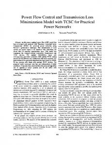
IV. APPLICATION OF THE FIREFLY ALGORITHM The process of incorporating the firefly algorithm for solving the optimal DG placement and sizing problem is shown in fig. 4 The test system for the case study is radial distribution system with IEEE 33 buses as shown in Figure 5.The total loads for this test system are 3.72 MW and 2.3 MVR.
Calculating voltages to each bus Calculate the sum of Power Losses
(12)
Where the first term is the current position of a firefly, the second term is used for considering a firefly’s attractiveness to light intensity seen by adjacent fireflies, and the third term is used for the random movement of a firefly in case there are not any brighter ones. The coefficient α is a randomization parameter determined by the problem of interest, while rand is a random number generator uniformly distributed in the space [0,1]. As we will see in this implementation of the algorithm, we will use β 0 =1.0, α ∈ [0, 1] and the attractiveness or absorption coefficient γ =1.0, which guarantees a quick convergence of the algorithm to the optimal solution [5].
Calculation of currents injected into the common bus
Objective function evaluation Ranking fireflies by their light intensity/objective Find the current best solution load flow data
Move all fireflies to the better locations (Updating fireflies)
No Iteration maximum
Yes Print results
End Fig 4. Flow of optimal allocation of DG using firefly algorithm
The substation voltage is 12.66 KV and the base of power is 10.00MVA. The test data of 33 bus Distribution system is available in papers [6] and [7] respectively. The results of FA are compared with those obtained by the method Shuffled Frog Leaping Algorithm SFLA [8].
(attractiveness) is 0.2. The scaling parameter is 0.25. Gamma (absorption coefficient) is 1 [9]. The Fig. 6 shows the Firefly convergence characteristic for cases 2 and 3 respectively. The Fig. 7 shows the bus voltages before and after installing DG. For the case 2, the minimum value of losses is 0.1167 MW with FA and is 0.1182 with Shuffled Frog Leaping Algorithm (SFLA). For case 3, the minimum value of losses obtained by FA is 0.0969 MW and by SFLA is 0.1054 MW. It also can be noted that the minimum bus voltage for cases 2 and 3 are 0.9398 pu and 0.9484 pu respectively by FA and 0.9384 pu and 0.9687 pu respectively by SFLA. The optimal location and size of DG in case 2 are bus 30 and 1.1904 MW respectively . For case 3, the optimal locations are at bus 14 and 30 with respectively sizes 0.6128 MW and 1.0131 MW . For the 33 bus system, the case 2 can reduce the total real power loss by 41%. For case 3, they can further reduce the real power loss by 51%. These results show the effectiveness of FA compared to SFLA. The comparison studies of these 3 cases are tabulated in Table 1.
1
Fig. 5.The schematic of a 33 bus radial distribution system
0.99
The following three cases to study the impact of DG installation on the system performance are considered: Case 1: Calculate the distribution network losses and minimum voltage without DG.
0.98 0.97 V o lt a g e ( p . u )
0.96
0.5 0.48
0.95
0.45
0.94
0.42 0.39
0.93
With one DG Without DG With tow DG
O b je c t if f u n t io n f (x )
0.36 0.92
0.33 0.3
0.91
0.27
With one DG With tow DG
0.24
0.9 5
0.21 0.18
10
15 20 Bus Number
25
30
Fig 7. Bus voltage before and after DG Installation
0.15 0.12 0.09 0.06 0.03 0
0
5
10
15 Iteration
20
25
30
Fig 6. Firefly convergence characteristic with one and tow DG
Case 2: Calculate the distribution network losses and minimum voltage with the one DG included once its optimal location and size are determined. Case 3: Calculate the distribution network losses and minimum voltage with the two DG included once its optimal location and size are determined. For FA parameters, population size is 20. The maximum iteration for FA algorithm is 30. Minimum value of beta
From the table 1, it can be seen that the result of location DG is similar with the Optimal Placement of DG in Radial Distribution Networks Using Shuffled Frog Leaping Algorithm (SFLA). For case 2 where the location for installing the DG is at bus 30 and for case 3 the optimal locations are at bus 14 and 30 respectively. The total line power losses obtained by FA are lower than obtained by Shuffled Frog Leaping Algrithm [8]. V. CONCLUSION In this paper, a Firefly algorithm (FA) for optimal placement and sizing of DG is efficiently minimizing the total real power loss and improve the voltage profile.
TABLE 1 COMPARISON RESULTS OF THE 33 BUS SYSTEM BETWEEN FIREFLY ALGORITHM AND SHUFFLED FROG LEAPING ALGRITHM FOR THREE CASES
Optimal location And size
0.1978
18
0.9039
-
-
SFLA
0.2277
18
0.8889
-
-
FA
0.1167
18
0.9398
1.1904
30
SFLA
0.1182
18
0.9384
1.1999
30
0.6128
14
1.0131
30
0.6022
14
1.0311
30
Allocation
voltage (p.u)
FA
Size(MW)
BUS Number
Real power Losses (MW)
Minimum bus voltage
Case 1
Case 2
FA
0.0969
18
0.9484
Case 3 SFLA
0.1054
18
0.9687
The proposed method was tested on IEEE 33-bus distribution system with three cases, without DG and with one and two DG included in the system. The performance of FA is good for solving the optimal location and sizing problem in the distribution system. The results show that incorporating the DG in the distribution system can reduce the total line power losses and improve the voltage profile. The total losses of the system in case with two DG integrated in the system are better than the case without and with one DG. The comparison with Shuffled Frog Leaping Algorithm (SFLA) [8] also has been conducted to see the performance of FA in solving the optimal allocation and sizing problems. REFERENCES [1] T. Ackermann, G. Anderson, L. Söder; “Distributed Generation: a Definition”, Electric Power System search, 2001, Vol. 57, pp.195-204. [2] W. El-Khattam, M.M.A. Salama; “Distributed generation technologies, definitions and benefits”, Electric Power Systems Research, 2004, Vol. 71, pp.119-128. [3] G.Pepermans, J.Driesen,D .Haeseldonckx, R.Belmans, W.D.haeseleer;“Distributed generation: definitions, benefits and issues”, Energy Policy, 2005, Vol. 33, pp.787-798. [4] P. P. Barker, R. W. de Mello; “Determining the Impact of Distributed Generation on Power Systems: Part 1–Radial Distribution Systems”, IEEE PES Summer Meeting, 2000, Vol.3, pp.1645-1656.
Yang, "Firefly algorithms for multimodal [5] X.-S. optimization,"Stochastic Algorithms: Foundation and Applications SAGA 2009, vol.5792, pp. 169-178, 2009 [6] J.Z. Zhu; “Optimal Reconfiguration of Electrical Distribution Network using the Refined Genetic Algorithm”, Electric Power Systems Research, 2002, Vol. 62, pp. 37-41. [7] M.A. Kashem, V. Ganapathy, G.B. Jasmon, M.I.Buhari; “A Novel Method for Loss Minimization in Distribution Networks” Proceeding of International Conference on Electric Utility Deregulation and Restructuring and Power Technologies, pp.251-255, 2000. [8] E. Afzalan, M. A. Taghikhani, M. Sedighizadeh “Optimal Placement and Sizing of DG in Radial Distribution Networks Using SFLA” International Journal of Energy Engineering 2012, 2(3): pp. 73-77 [9] M. H. Sulaiman, M.W. Mustafa.; A. Azmi; O. Aliman; S. R. Abdul Rahim; “ Optimal Allocation and Sizing of Distributed Generation in Distribution System via Firefly Algorithm ” Power Engineering and Optimization Conference (PEDCO) Melaka, Malaysia, 2012, pp. 84-89