First-order vs. higher-order modification in distributional semantics Gemma Boleda Linguistics Department University of Texas at Austin
[email protected]
Eva Maria Vecchi Center for Mind/Brain Sciences University of Trento
[email protected]
Miquel Cornudella and Louise McNally Departament de Traducci´o i Ci`encies del Llenguatge Universitat Pompeu Fabra
[email protected],
[email protected] Abstract Adjectival modification, particularly by expressions that have been treated as higherorder modifiers in the formal semantics tradition, raises interesting challenges for semantic composition in distributional semantic models. We contrast three types of adjectival modifiers – intersectively used color terms (as in white towel, clearly first-order), subsectively used color terms (white wine, which have been modeled as both first- and higher-order), and intensional adjectives (former bassist, clearly higher-order) – and test the ability of different composition strategies to model their behavior. In addition to opening up a new empirical domain for research on distributional semantics, our observations concerning the attested vectors for the different types of adjectives, the nouns they modify, and the resulting noun phrases yield insights into modification that have been little evident in the formal semantics literature to date.
1
Introduction
One of the most appealing aspects of so-called distributional semantic models (see Turney and Pantel (2010) for a recent overview) is that they afford some hope for a non-trivial, computationally tractable treatment of the context dependence of lexical meaning that might also approximate in interesting ways the psychological representation of that meaning (Andrews et al., 2009). However, in order to have a complete theory of natural language meaning, these models must be supplied with or connected to a compositional semantics; otherwise,
we will have no account of the recursive potential that natural language affords for the construction of novel complex contents. In the last 4-5 years, researchers have begun to introduce compositional operations on distributional semantic representations, for instance to combine verbs with their arguments or adjectives with nouns (Erk and Pad´o, 2008; Mitchell and Lapata, 2010; Baroni and Zamparelli, 2010; Grefenstette and Sadrzadeh, 2011; Socher et al., 2011)1 . Although the proposed operations have shown varying degrees of success in a number of tasks such as detecting phrase similarity and paraphrasing, it remains unclear to what extent they can account for the full range of meaning composition phenomena found in natural language. Higher-order modification (that is, modification that cannot obviously be modeled as property intersection, in contrast to firstorder modification, which can) presents one such challenge, as we will detail in the next section. The goal of this paper is twofold. First, we examine how the properties of different types of adjectival modifiers, both in isolation and in combination with nouns, are represented in distributional models. We take as a case study three groups of adjectives: 1) color terms used to ascribe true color properties (referred to here as intersective color terms), as prototypical representative of first-order modifiers; 2) color terms used to ascribe properties other than simple color (here, subsective color terms), as representatives of expressions that could in principle 1 In a complementary direction, Garrette et al. (2011) connect distributional representations of lexical semantics to logicbased compositional semantics.
1223 Proceedings of the 2012 Joint Conference on Empirical Methods in Natural Language Processing and Computational Natural c Language Learning, pages 1223–1233, Jeju Island, Korea, 12–14 July 2012. 2012 Association for Computational Linguistics
be given a well-motivated first-order or higher-order analysis; and 3) intensional adjectives (e.g. former), as representative of modifiers that arguably require a higher-order analysis. Formal semantic models tend to group the second and third groups together, despite the existence of some natural language data that questions this grouping. However, our results show that all three types of modifiers behave differently from each other, suggesting that their semantic treatment needs to be differentiated. Second, we test how five different composition functions that have been proposed in recent literature fare in predicting the attested properties of nominals modified by each type of adjective. The model by Baroni and Zamparelli (2010) emerges as a suitable model of adjectival composition, while multiplication and addition shed mixed results. The paper is structured as follows. Section 2 provides the necessary background on the semantics of adjectival modification. Section 3 presents the methods used in our study. Section 4 describes the characteristics of the different types of adjectival modification, and Section 5, the results of the composition operations. The paper concludes with a general discussion of the results and prospects for future work.
2
The semantics of adjectival modification
Accounting for inference in language is an important concern of semantic theory. Perhaps for this reason, within the formal semantics tradition the most influential classification of adjectives is based on the inferences they license (see (Parsons, 1970) and (Kamp, 1975) for early discussion). We very briefly review this classification here. First, so called intersective adjectives, such as (the literally used) white in white dress, yield the inference that both the property contributed by the adjective and that contributed by the noun hold of the individual described; in other words, a white dress is white and is a dress. The semantics for such modifiers is easily characterized in terms of the intersection of two first-order properties, that is, properties that can be ascribed to individuals. On the other extreme, intensional adjectives, such as former or alleged in former/alleged criminal, do not license the inference that either of the properties holds of the individual to which the modified nom1224
inal is ascribed. Indeed, such adjectives cannot be used as predicates at all: (1) ??The criminal was former/alleged. The infelicity of (1) is generally attributed to the fact that these adjectives do not describe individuals directly but rather effect more complex operations on the meaning of the modified noun. It is for this reason that these adjectives can be considered higher-order modifiers: they behave as properties of properties. Though rather abstract, the higher-order analysis is straightforwardly implementable in formal semantic models and captures a range of linguistic facts successfully. Finally, subsective adjectives such as (the nonliterally-used) white in white wine, consitute an intermediate case: they license the inference that the property denoted by the noun holds of the individual being described, but not the property contributed by the adjective. That is, white wine is not white but rather a color that we would probably call some shade of yellow. This use of color terms, in general, is distinguished primarily by the fact that color serves as a proxy for another property that is related to color (e.g. type of grape), though the color in question may or may not match the color identified by the adjective on the intersective use (see (G¨ardenfors, 2000) and (Kennedy and McNally, 2010) for discussion and analysis). The effect of the adjective, rather than to identify a value for an incidental COLOR attribute of an object, is often to characterize a subclass of the class described by the noun (white wine is a kind of wine, brown rice a kind of rice, etc.). This use of color terms can be modeled by property intersection in formal semantic models only if the term is previously disambiguated or allowed to depend on context for its precise denotation. However, it is easily modeled if the adjective denotes a (higher-order) function from properties (e.g. that denoted by wine) to properties (that denoted by white wine), since the output of the function denoted by the color term can be made to depend on the input it receives from the noun meaning. Nonetheless, there is ample evidence in natural language that a firstorder analysis of the subsective color terms would be preferable, as they share more features with pred-
icative adjectives such as happy than they do with adjectives such as former. The trio of intersective color terms, subsective color terms, and intensional adjectives provides fertile ground for exploring the different composition functions that have been proposed for distributional semantic representations. Most of these functions start from the assumption that composition takes pairs of vectors (e.g. a verb vector and a noun vector) and returns another vector (e.g. a vector for the verb with the noun as its complement), usually by some version of vector addition or multiplication (Erk and Pad´o, 2008; Mitchell and Lapata, 2010; Grefenstette and Sadrzadeh, 2011). Such functions, insofar as they yield representations which strengthen distributional features shared by the component vectors, would be expected to model intersective modification. Consider the example of white dress. We might expect the vector for dress to include non-zero frequencies for words such as wedding and funeral. The vector for white, on the other hand, is likely to have higher frequencies for wedding than for funeral, at least in corpora obtained from the U.S. and the U.K. Combining the two vectors with an additive or multiplicative operation should rightly yield a vector for white dress which assigns a higher frequency to wedding than to funeral. Additive and multiplicative functions might also be expected to handle subsective modification with some success because these operations provide a natural account for how polysemy is resolved in meaning composition. Thus, the vector that results from adding or multiplying the vector for white with that for dress should differ in crucial features from the one that results from combining the same vector for white with that for wine. For example, depending on the details of the algorithm used, we should find the frequencies of words such as snow or milky weakened and words like straw or yellow strengthened in combination with wine, insofar as the former words are less likely than the latter to occur in contexts where white describes wine than in those where it describes dresses. In contrast, it is not immediately obvious how these operations would fare with intensional adjectives such as former. In particular, it is not clear what specific distributional features of the adjective would capture the effect that the ad1225
jective has on the meaning of the resulting modified nominal. Interestingly, recent approaches to the semantic composition of adjectives with nouns such as Baroni and Zamparelli (2010) and Guevara (2010) draw on the classical analysis of adjectives within the Montagovian tradition of formal semantic theory (Montague, 1974), on which they are treated as higher order predicates, and model adjectives as matrices of weights that are applied to noun vectors. On such models, the distributional properties of observed occurrences of adjective-noun pairs are used to induce the effect of adjectives on nouns. Insofar as it is grounded in the intuition that adjective meanings should be modeled as mappings from noun meanings to adjective-noun meanings, the matrix analysis might be expected to perform better than additive or multiplicative models for adjective-noun combinations when there is evidence that the adjective denotes only a higher-order property. There is also no a priori reason to think that it would fare more poorly at modeling the intersective and subsective adjectives than would additive or multiplicative analyses, given its generality. In this paper, we present the first studies that we know of that explore these expectations.
3
Method
We built a semantic space and tested the composition functions as specified in what follows. 3.1
Semantic space
The semantic space we used for our experiments consists of a matrix where each row vector represents an adjective, noun or adjective-noun phrase (henceforth, AN). We first introduce the source corpus, then the vocabulary that we represent in the space, and finally the procedure to build the vectors representing the vocabulary items from corpus data. 3.1.1 Source corpus Our source corpus is the concatenation of the ukWaC corpus2 , a mid-2009 dump of the English Wikipedia3 and the British National Corpus4 . The corpus is tokenized, POS-tagged and lemmatized 2
http://wacky.sslmit.unibo.it/ http://en.wikipedia.org 4 http://www.natcorp.ox.ac.uk/ 3
with TreeTagger (Schmid, 1995) and contains about 2.8 billion tokens. We extracted all statistics at the lemma level, ignoring inflectional information. 3.1.2 Vocabulary The core vocabulary of the semantic space consists of the 8K most frequent nouns and the 4K most frequent adjectives from the corpus. By crossing the set of 700 most frequent adjectives (reduced to 663 after removing questionable items like above, less and very) and the 4K most frequent nouns and selecting those ANs that occured at least 100 times in the corpus, we obtained a set of 179K ANs that we added to the semantic space, for a total of 191K rows. These ANs were used for training the linear models as well as for providing a basis for the analysis of the results. 3.1.3 Semantic space parameters The dimensions (columns) of our semantic space are the top 10K most frequent content words in the corpus (nouns, adjectives, verbs and adverbs), excluding the 300 most frequent words of all parts of speech. For each word or AN, we collected raw cooccurrence counts by recording their sentenceinternal co-occurrence with each of words in the dimensions. The counts were then transformed into Local Mutual Information (LMI) scores, an association measure that closely approximates the commonly used Log-Likelihood Ratio but is simpler to compute (Evert, 2005). Specifically, given a row element r, a column element c and a counting function C(r, c), then LM I = C(r, c) · log
C(r, c)C(∗, ∗) C(r, ∗)C(∗, c)
(1)
where C(r, c) is how many times r cooccurs with c, C(r, ∗) is the total count of r, C(∗, c) is the total count of c, and C(∗, ∗) is the cumulative cooccurrence count of any r with any c. The dimensionality of the space was reduced using Singular Value Decomposition (SVD), as in Latent Semantic Analysis and related distributional semantic methods (Landauer and Dumais, 1997; Rapp, 2003; Sch¨utze, 1997). Both LMI and SVD were used for the core vocabulary, and the AN vectors were computed based on the values for the 1226
core vocabulary. All of the results discussed in the article are based on the SVD-reduced space, because it yielded consistently better results, except for those involving multiplicative composition, which was carried out on the non-reduced model because SVD reduction introduces negative values for the latent dimensions used for the reduced space. Some of the parameters of the space and composition functions were set based on performance on independent word similarity and AN similarity tasks (Rubenstein and Goodenough, 1965; Mitchell and Lapata, 2010). In addition to LMI, we tested the performance using log-transformed frequencies and found very poor performance in the aforementioned tasks. The number of latent dimensions for the SVD-reduced space was set at 300 after testing the performance using 300, 600 and 900 latent dimensions. In the discussion, we use the cosine of two vectors as a measure of similarity. This is the most common choice in related work, as it has shown to be robust across different tasks and settings, though other options (in particular, measures that are not symmetric or do not normalize) could be explored (Widdows, 2004). 3.2
Composition models
The experiments described below were carried out using five compositional methods that have been explored in recent studies of compositionality in distributional semantic spaces (Mitchell and Lapata, 2010; Guevara, 2010; Baroni and Zamparelli, 2010). For each function, we define p as the composition of the adjective vector, u, and the noun vector, v, a nomenclature that follows Mitchell and Lapata (2010). Additive (add) AN vectors were obtained by summing the corresponding adjective and noun vectors. We also explored the effects of the additive model with normalized component adjective and noun vectors (addn ). p=u+v
(2)
Multiplicative (mult) AN vectors were obtained by component-wise multiplication of the adjective and noun vectors in the non-reduced semantic space. p=u v
(3)
Dilation (dl) AN vectors were obtained by calculating the dot products of u·u and u·v and stretching v by a factor λ (in our case, 16.7) in the direction of u (Clark et al., 2008; Mitchell and Lapata, 2010). The effect of this operation is to “stretch” the head vector v (noun, in our case) in the direction of the modifying vector u (adjective). p = (u · u)v + (λ − 1)(u · v)
(4)
The factor λ was selected based on the optimal parameters presented in Mitchell and Lapata (2010). We tested both reported values (16.7 and 2.2) and found λ = 16.7 to perform better in terms of rank of observed equivalent (see Section 5). The preceding functions produce an AN vector from the component A and N vectors. The remaining two functions do not use the vector for the adjective, but learn a matrix representation for it. The composed AN vector is obtained by multiplying the matrix by the noun vector. The general equation for the two functions is the following, where B is a matrix of weights that is multiplied by the noun vector v to produce the AN vector p. p = Bv
(5)
In the linear map (lim) approach proposed by Guevara (2010), one single matrix B is learnt that represents all adjectives. An AN vector is obtained by multiplying the weight matrix by the concatenation of the adjective and noun vectors, so that each dimension of the generated AN vector is a linear combination of dimensions of the corresponding adjective and noun vectors. In our implementation, B is an 300 x 300 weight matrix representing an adjective, and v is a 300-dimension noun vector. Following Guevara (2010), we estimate the coefficients of the equation using (multivariate) partial least squares regression (PLSR) as implemented in the R pls package (Mevik and Wehrens, 2007), setting the latent dimension parameter of PLSR to 300. This value was chosen after testing values 100, 200 and 300 on the AN similarity tasks (Mitchell and Lapata, 2010). Coefficient matrix estimation is performed by feeding PLSR a set of input-output examples, where the input is given by concatenated adjective and noun vectors, and the output is the vector of the corresponding AN directly extracted from our 1227
semantic space. The matrix is estimated using a random sample of 2.5K adjective-noun-AN tuples.5 In the adjective-specific linear map (alm) model, proposed by Baroni and Zamparelli (2010), a different matrix B is learnt for each adjective. The weights of each of the rows of the weight matrix are the coefficients of a linear equation predicting the values of one of the dimensions of the normalized AN vector as a linear combination of the dimensions of the normalized component noun. The linear equation coefficients are estimated again using PLSR, and in the present implementation we use ridge regression generalized cross-validation (GCV) to automatically choose the optimal ridge parameter for each adjective (Golub et al., 1979). This procedure drastically outperforms setting a fixed number of dimensions. The model is trained on all NAN vector pairs available in the semantic space for each adjective, and range from 100 to over 1K items across the adjectives we tested. 3.3
Datasets
We built two datasets of adjective-noun phrases for the present research, one with color terms and one with intensional adjectives.6 Color terms. This dataset is populated with a randomly selected set of adjective-noun pairs from the space presented above. From the 11 colors in the basic set proposed by Berlin and Kay (1969), we cover 7 (black, blue, brown, green, red, white, and yellow), since the remaining (grey, orange, pink, and purple) are not in the 700 most frequent set of adjectives in the corpora used. From an original set of 412 ANs, 43 were manually removed because of suspected parsing errors (e.g. white photograph, for black and white photograph) or because the head noun was semantically transparent (white variety). The remaining 369 ANs were tagged independently by the second and fourth authors of this paper, both native English speaker linguists, as intersective (e.g. white towel), subsective (e.g. white wine), or idiomatic, i.e. compositionally non-transparent (e.g. black hole). They were allowed the assignment of at 5
2.5K ANs is the upper bound of the software package used. Available at http://dl.dropbox.com/u/513347/ resources/data-emnlp2012.zip. See Bruni et al. (to appear) for an analysis of the color term dataset from a multimodal perspective. 6
most two labels in case of polysemy, for instance for black staff for the person vs. physical object senses of the noun or yellow skin for the race vs. literally painted interpretations of the AN. In this paper, only the first label (most frequent interpretation, according to the judges) has been used. The κ coefficient of the annotation on the three categories (first interpretation only) was 0.87 (conf. int. 0.82-0.92, according to Fleiss et al. (1969)), observed agreement 0.96.7 There were too few instances of idioms (17) for a quantitative analysis of the sort presented here, so these are collapsed with the subsective class in what follows.8 The dataset as used here consists of 239 intersective and 130 subsective ANs. Intensional adjectives. The intensional dataset contains all ANs in the semantic space with a preselected list of 10 intensional adjectives, manually pruned by one of the authors of the paper to eliminate erroneous examples and to ensure that the adjective was being intensionally used. Examples of the ANs eliminated on these grounds include past twelve (cp. accepted past president), former girl (probably former girl friend or similar), false rumor (which is a real rumor that is false, vs. e.g. false floor, which is not a real floor), or theoretical work (which is real work related to a theory, vs. e.g. theoretical speed, which is a speed that should have been reached in theory). Other AN pairs were excluded on the grounds that the noun was excessively vague (e.g. past one) or because the AN formed a fixed expression (e.g. former USSR). The final dataset contained 1,200 ANs, distributed as follows: former (300 examples), possible (244), future (243), potential (183), past (87), false (44), apparent (39), artificial (36), likely (18), theoretical (6).9 Table 1 contains examples of each type of AN we are considering. 7
Code for the computation of inter-annotator agreement by Stefan Evert, available at http://www.collocations. de/temp/kappa_example.zip. 8 An alternative would have been to exclude idiomatic ANs from the analysis. 9 Alleged, one of the most prototypical intensional adjectives, is not considered here because it was not among the 700 most frequent adjectives in the space. We will consider it in future work.
1228
Intersective white towel black sack green coat red disc blue square
Subsective white wine black athlete green politics red ant blue state
Intensional artificial leg former bassist likely suspect possible delay theoretical limit
Table 1: Example ANs in the datasets.
4
Observed vectors
We began by exploring the empirically observed vectors for the adjectives (A), nouns (N), and adjective-noun phrases (AN) in the datasets, as they are represented in the semantic space. Note that we are working with the AN vectors directly harvested from the corpora (that is, based on the cooccurrence of, say, the phrase white towel with each of the 10K words in the space dimensions), without doing any composition. AN vectors obtained by composition will be examined in the following section. Though observed AN vectors should not be regarded as a gold standard in the sense of, for instance, Machine Learning approaches, because they are typically sparse10 and thus the vectors of their component adjective and noun will be richer, they are still useful for exploration and as a comparison point for the composition operations (Baroni and Lenci, 2010; Guevara, 2010). Figure 1 shows the distribution of the cosines between A, N, and AN vectors with intensional adjectives (I, white box), intersective uses of color terms (IE, lighter gray box), and subsective uses of color terms (S, darker gray box). In general, the similarity of the A and N vectors is quite low (cosine < 0.2, left graph of Figure 1), and much lower than the similarities between both the AN and A vectors and the AN and N vectors. This is not surprising, given that adjectives and nouns describe rather different sorts of things. We find significant differences between the three types of adjectives in the similarity between AN and A vectors (middle graph of Figure 1). The adjective and adjective-noun phrase vectors are nearer for 10
The frequency of the adjectives in the datasets range from 3.5K to 3.7M, with a median frequency of 109,114. The nouns range from 4.9K to 2.5M, with a median frequency of 148,459. While the frequency of the ANs range from 100 to 18.5K, with a median frequency of 239.
cos(AN,A)
cos(AN,N)
●
1.0
1.0
1.0
cos(A,N) ● ●
●
0.8
● ●
0.8
0.8
● ● ●
●
● ● ● ● ● ● ● ●
● ● ●
0.6
●
0.6
0.6
● ● ●
●
●
●
0.4 0.2
0.0
0.0
0.0
0.2
0.2
●
0.4
0.4
● ●
I
L
N
I
L
N
I
L
N
Figure 1: Cosine distance distribution in the different types of AN. We report the cosines between the component adjective and noun vectors (cos(A,N)), between the observed AN and adjective vectors (cos(AN,A)), and between the observed AN and noun vectors (cos(AN,N)). Each chart contains three boxplots with the distribution of the cosine scores (y-axis) for the intensional (I), intersective (IE), and subsective (S) types of ANs. The boxplots represent the value distribution of the cosine between two vectors. The horizontal lines in the rectangles represent the first quartile, median, and third quartile. Larger rectangles correspond to a more spread distribution, and their (a)symmetry mirrors the (a)symmetry of the distribution. The lines above and below the rectangle stretch to the minimum and maximum values, at most 1.5 times the length of the rectangle. Values outside this range (outliers) are represented as points.
intersective uses than for subsective uses of color terms, a pattern that parallels the difference in the distance between component A and N vectors. Since intersective uses correspond to the prototypical use of color terms (a white dress is the color white, while white wine is not), the greater similarity for the intersective cases is unsurprising – it suggests that in the case of subsective adjectival modifiers, the noun “pulls” the AN further away from the adjective than happens with the cases of intersective modification. This is compatible with the intuition (manifest in the formal semantics tradition in the treatment of subsective adjectives as higher-order rather than firstorder, intersective modifiers) that the adjective’s effect on the AN in cases of subsective modification depends heavily on the interpretation of the noun with which the adjective combines, whereas that is less the case when the adjective is used intersectively. As for intensional adjectives, the middle graph shows that their AN vectors are quite distant from the corresponding A vectors, in sharp contrast to what we find with both intersective and subsective 1229
color terms. We hypothesize that the results for the intensional adjectives are due to the fact that they cannot plausibly be modeled as first order attributes (i.e. being potential or apparent is not a property in the same sense that being white or yellow is) and thus typically do not restrict the nominal description per se, but rather provide information about whether or when the nominal description applies. The result is that intensional adjectives should be even weaker than subsectively used adjectives, in comparison with the nouns with which they combine, in their ability to “pull” the AN vector in their direction. Note, incidentally, that an alternative explanation, namely that the effect mentioned could be due to the fact that most nouns in the intensional dataset are abstract and that adjectives modifying abstract nouns might tend to be further away from their nouns altogether, is ruled out by the comparison between the A and N vectors: the A-N cosines of the intensional and intersective ANs are similar. We thus conclude that here we see an effect of the type of modification involved. An examination of the average distances among
the nearest neighbors of the intensional and of the color adjectives in the distributional space supports our hypothesized account of their contrasting behaviors. We predict that the nearest neighbors are more dispersed for adjectives that cannot be modeled as first-order properties (i.e., intensional adjectives), than for those that can (here, the color terms). We find that the average cosine distance among the nearest ten neighbors of the intensional adjectives is 0.74 with a standard deviation of 0.13, which is significantly lower (t-test, p