First-Principles Computation of YVO3; Combining Path-Integral ...
Recommend Documents
We report a comprehensive neutron diffraction study of the crystal structure and .... were grown using the crucible-free floating zone technique as described ...
Due to the oxygen deficiency at one of the apical oxygen sites, the Fe-atom at 4i(0,y,0) is shifted out of the plane [or from the ideal value y = ¼ to 0.253(1)], which ...
LEM integrates two modes of operation: Machine Learning mode, which ..... conventional evolutionary algorithm, ES, that we re-implemented in C++ from an ...
bDepartment of Chemical Engineering, National Taiwan University of ... spectroscopy and first principles electronic structure computations indicate that Ni and ...
To enable this study to be carried out, such a sequence of nested multi-block ... 1(a) Domain decomposition around the DLR-F4 wing body configuration using.
Birkhoff decomposition of doubly stochastic matrices, an arbitrary .... a 2 Ã 2 permutation matrix. ..... because commuting a diagonal matrix with a permutation.
Mar 20, 2008 - ... of the Pbnm and P21/b crystal systems are given in the upper left corner of each figure. arXiv:0803.3046v1 [cond-mat.str-el] 20 Mar 2008 ...
REQUIREMENTS FOR THE DEGREE ... Faculty Fellow of Computer Science ... code very quickly, a useful feature for compilers that stress compilation speed over ... track of what is important in computer science, and helped me to distinguish ...
considered; it is shown numerically that, for a xed spatial truncation, the error in the truncation scales with .... ODE codes such as Homcont, see. 8, 10], can ... the explicit construction of this projection for semilinear elliptic equations in 27,
[email protected]. 1. Motivation ... body of work in security usability is growing, but much of it is adhoc and ... Modification Using Guided Inference. Submitted to ...
submatrix of n à n matrix A which is composed of rows and columns indexed by 1 ⤠k1 ..... We implement Algorithm 4.1 in the package Mathematica 8.0 and.
May 1, 2017 - a Saturday, a Sunday, or a legal holiday as defined in T.C.A. § 15-1-101, or, when the act to be done is
Reviews of books in areas related to computational mathematics are also ...
Steffen Börm and Stefan A. Sauter, BEM with linear complexity for the ..... AMS
website, corrections may be made to the paper by submitting a traditional ....
ERNST HAIRER
... of Computation. Exploring the Power of Computing ... The book covers the
traditional topics of formal languages and automata and complexity classes but
also ...
Oct 14, 2008 ... Theory of Computation. Solutions to Homework 1. Problem 1. Briefly describe a
Turing machine that accepts a string x ∈. {0,1}∗ if and only if x ...
1. CHAPTER 17. Theory of Computation. (Solutions to Odd-Numbered Problems)
. Review Questions. 1. The three statements in our Simple Language are the ...
Keywords: Geometric moments; moment invariants; fast computation of .... Comparison of values of the function xp and its Schlick's approximation for different.
Why not just use von-Neumann computing (C,. Java, â¦) ... Erich Gamma, Richard Helm, Ralph Johnson, John Vlissides: Design Patterns, Addision-. Wesley ...
At the 0th clock tick, NS1 and NS2 are 0. For all further clock ticks, the outputs of the neurons are NS1 and NS2 (for neuron 1 and 2 respectively). c) EXS is the ...
aggregate model might be to combine the information in the disaggregate variables first, ... uncertainty are the primary sources of differences in forecast accuracy ... shows that aggregating forecasts by component does not necessarily help to .... p
Sep 29, 2014 -
Dec 7, 2005 ... computer games. For example, the ESP Game, introduced in this thesis, is an
enjoyable online game — many people play over 40 hours a ...
SQL Server 2005 and VB.Net on Surah Al-Baqarah. The ..... [33] M. Shoaib, M.N. Yasin, K. Hikmat Ullah, M.I. Saeed, and M.S.H.. Khiyal, âRelational WordNet ...
First-Principles Computation of YVO3; Combining Path-Integral ...
Sep 30, 2006 - by using the local muffin-tin orbital basis is applied to derive the whole band structure. The electron degrees of freedom far from the Fermi level ...
First-Principles Computation of YVO3; Combining Path-Integral Renormalization Group with Density-Functional Approach Yuichi Otsuka1,2 1
∗ †
and Masatoshi Imada1,2,3
Institute for Solid State Physics, University of Tokyo, Kashiwanoha, Kashiwa, Chiba 277-8581, Japan 2
3
PRESTO, Japan Science and Technology Agency, 4-1-8 Honcho, Kawaguchi, Saitama, Japan Depertment of Applied Physics, University of Tokyo, 7-3-1 Hongo Bunkyo-ku, Tokyo 113-8656, Japan We investigate the electronic structure of the transition-metal oxide YVO3 by a hybrid first-principles scheme. The density-functional theory with the local-density-approximation by using the local muffin-tin orbital basis is applied to derive the whole band structure. The electron degrees of freedom far from the Fermi level are eliminated by a downfolding procedure leaving only the V 3d t2g Wannier band as the low-energy degrees of freedom, for which a low-energy effective model is constructed. This low-energy effective Hamiltonian is solved exactly by the path-integral renormalization group method. It is shown that the ground state has the G-type spin and the C-type orbital ordering in agreement with experimental indications. The indirect charge gap is estimated to be around 0.7 eV, which prominently improves the previous estimates by other conventional methods. KEYWORDS: First-principles
calculation,
density-functional
theory,
local-density-
approximation, path-integral renormalization group, transition-metal oxide, Mott transition, orbital order, charge gap
1. Introduction Recent intensive studies have revealed that strongly correlated electron systems exhibit a variety of distinguished physical properties.1 Basic aspects of the correlation effects have been studied mainly by simplified models, such as the Hubbard, and Heisenberg models. For example, at least some essence of the Mott transition, which is widely seen in the strongly correlated electron systems, is believed to be captured by the single-band Hubbard model. However, if we focus on a variety of physical properties in real materials, many challenging issues are found beyond the simplified models. Especially in the systems where spin and orbital are coupled, rich structure and various phenomena have attracted much interest. When the strong Coulomb interaction suppresses charge fluctuations, spin and orbital degrees of freedom play a crucial role. In order to understand such realistic and complex systems, computational ∗
Present address: Synchrotron Radiation Research Center, Japan Atomic Energy Research Institute, Hyogo
methods from the first principles offer promising approaches because of their ability to treat charge, spin and orbital degrees of freedom on equal footing with full fluctuation effects taken into account. Computational methods for electronic structure calculations are roughly classified into two categories. One is based on the density-functional theory (DFT) supplemented, for example, with the local-density-approximation (LDA).2, 3 Since the LDA costs less computation time, this scheme has proven its advantage in calculating electronic structure of real materials. However, the LDA essentially ignores spatial and dynamical fluctuations which are relevant in the strongly correlated systems. In addition, the LDA in general underestimates the charge gap. The other approach is based on the wave function scheme. The Hartree-Fock (HF) method often gives a good starting point to discuss competition among ordered states, while it tends to overestimate the charge gap. The HF approximation itself is a rather crude one, where spatial and temporal correlations are ignored. However, one can improve the accuracy systematically within the wave function scheme by expanding basis set, for instance, by introducing configuration interaction or by path-integral renormalization-group (PIRG) methods.4 The method along this line tends to need much longer computational time, which prevents us from applying it directly to real materials. Recently, a hybrid method called DFT-PIRG which combines the DFT with a wave function method, namely PIRG has been proposed.5 The DFT is utilized to first obtain the overall band structure extending to the energy scale far from the Fermi level. Then the downfolding procedure eliminates the high-energy degrees of freedom far from the Fermi level by the renormalization process. After this downfolding process, an effective model for the low-lying electronic structure is obtained, which is solved exactly by a low-energy solver. The PIRG method is a promising choice for a low-energy solver because it allows us to treat spatial and dynamical fluctuations in a controllable way. It has indeed been applied to Sr2 VO4 5, 6 and has reproduced the basic experimental properties including the fact that this compound is located just on the verge of the Mott transition with a tiny but nonzero gap amplitude (. 0.1eV). In the present work, we study YVO3 as another example of the charge-spin-orbital coupled system by the DFT-PIRG method. YVO3 belongs to the family of transition-metal oxides with two valence electrons in the 3d orbitals (t2g manifold). The lattice structure is an orthorhombically distorted perovskite with the space group P bnm (four vanadium sites in a unit cell) at room temperatures. The GdFeO3 type distortion, rotation and tilting of the VO6 octahedra are present, where the reduced V-O-V angle makes the narrow t2g bands. With lowering the temperature, it undergoes two successive phase transitions in both spin and orbital sectors. First, the G-type orbital ordering (OO) appears at 200K with a structural change to the P 21 /a symmetry, where a site with the dxy and dyz orbitals occupied and one with the the dxy and dzx are alternatively arranged in
2/17
J. Phys. Soc. Jpn.
Full Paper
three dimensions. The magnetic structure shows the C-type spin ordering (SO) below 116K, where spins are aligned antiferromagnetically in the a-b plane and ferromagnetically along the c-axis. With further lowering the temperature, the SO and OO simultaneously change at 77K, and the ground-state is the C-type OO with the G-type SO.7, 8 The crystal structure recovers the P bnm symmetry as illustrated in Fig. 1. In the charge sector, YVO3 is a typical Mott insulator with a large charge gap (∼ 1eV). This is partly attributed to a large GdFeO3 type distortion, which reduces the band width effectively. In addition, coupling to Jahn-Teller distortions is important in determining the orbital states.
Fig. 1. (Color online): Illustration of the P bnm orthorhombic crystal structure of YVO3 . Each V atom (large red sphere) is octahedrally surrounded by O atoms (small blue spheres). Other (light yellow) spheres represents Y atoms.
The relation between the SO and the OO has been studied by the unrestricted HF approximation.9, 10 Although the HF result explains the spin and orbital orders in the ground-state consistently with the experiments, the magnitude of the charge gap is largely overestimated (∼ 3.4eV) compared to the experimental value (∼ 1eV). From the first-principles calculations, the 3/17
J. Phys. Soc. Jpn.
Full Paper
local spin density approximation (LSDA) and the generalized gradient approximation (GGA) have been applied with the full-potential linearized augmented-plane-wave method.11, 12 The LSDA results have shown the metallic ground state. On the other hand, the ground state is insulating with GGA, but it failed to reproduce the correct SO and OO. In addition, the gap amplitude is underestimated (0.009eV). The LDA+U method has succeeded in describing the correct ground state.12, 13 However, aside from the issue of avoiding the double counting of the Coulomb interaction generally known in LDA+U calculation, this ground state is obtained by adjusting the parameter U to reproduce the experimental band gap. It is desired to estimate the screened Coulomb interaction itself from the first principle. In addition, it is also important to go beyond the single-Slater-determinant approximation to examine effects of quantum fluctuations accurately, and to estimate spatial and temporal fluctuations from the first principles. This is because orbital-spin fluctuations may seriously alter the ground state through strong correlations combined with quantum fluctuations. The purpose of the present work is to study the ground state of YVO3 from the firstprinciples calculation at a quantitative level. We will discuss how the SO and OO are reproduced with the DFT-PIRG scheme and estimate the charge gap. The basic procedures are the same as the case of Sr2 VO4 . Readers are referred to refs. 5, 6 for more detailed description of this scheme. Here we note that the target materials are quite different, while the procedures are similar. In contrast to Sr2 VO4 , YVO3 is a cubic perovskite with the GdFeO3 -type distortion, where its isotropic three dimensionality or mixing between t2g orbitals may show different aspects. The inter-orbital Coulomb interaction and the Hund’s rule coupling are considered to be more effective for the 3d2 configuration of YVO3 . Furthermore, YVO3 has much larger Mott gap (∼ 1eV). To examine the applicability of the DFT-PIRG method, it is desired to test whether it works in such completely different systems. In Sec. II, we derive the effective low-energy model. In Sec.III, the Hartree-Fock solution to this model is considered. We discuss results of the PIRG calculation in Sec. IV. Section V is devoted to summary. 2. Constructing Effective Model In many cases of the strongly correlated electron systems, the bands close to the Fermi level are relatively narrow and well separated from the bands far from the Fermi level. In fact, for the transition metal oxides, the 3d bands are mostly responsible for the low-energy excitations. Compared to the width of the 3d bands, other bands are located far from the Fermi level. Furthermore, if the crystal-field splitting is strong, it may be sufficient to consider only either eg or t2g bands for the low-energy degrees of freedom. This hierarchy structure in energy enables us to treat the system in a hybrid scheme. The electron correlation effects and dynamical fluctuations are important near the Fermi level, whereas the electronic structure far from the Fermi level is expected to be well repro-
4/17
J. Phys. Soc. Jpn.
Full Paper
duced by LDA. Therefore, in the first step of our hybrid scheme, the whole electronic structure is calculated from the density functional approach by employing LDA based on the linear muffin-tin orbital (LMTO) method.14, 15 The LDA enables us to calculate the whole electronic structure within the presently available computer power. Then we eliminate the electronic degrees freedom far from the Fermi level. This is done by the renormalization (downfolding) procedure, where the electron correlation effects are properly considered in the calculation of the screening and self-energy effects. After the downfolding procedure, the low-energy degrees of freedom isolated near the Fermi level are extracted in the effective Hamiltonian, which will be solved accurately in the PIRG method. Let us explain the whole procedure developed in the literature5, 6 by extending it specifically for the present compound YVO3 . At first, we compute the LDA band structure from the LMTO basis. Since YVO3 has sufficiently large crystal-field splitting (∼ 0.1eV) due to a large Jahn-Teller distortion, we focus on three low-energy bands which mainly consist of the 3d t2g orbitals. The whole Hilbert space is now spanned by the LDA basis functions for the LMTO t2g bands {|di} and the set of the rest basis {|ri}. Then we eliminate the subspace {|ri} and reduce the Hilbert space to the subspace which only consists of the set {|di}.5, 16 The Hamiltonian matrix is now spanned only within this restricted Hilbert subspace, which provides us with the low-energy tight-binding effective Hamiltonian defined on the Wannier basis for the 3d t2g bands. Note that the band structure of the effective tight-binding Hamiltonian defined only on the low-energy subspace well reproduces the t2g part of LDA bands computed from the whole LMTO basis as is illustrated in Fig. 2.
Fig. 2. (Color online): Comparison of the band structure of 3d t2g orbitals computed from LMTO calculations (solid light blue lines) with the downfolded tight-binding model (dashed-dotted brown lines) for YVO3 .
Next, the parameter values for the final effective low-energy Hamiltonian for the 3d t2g Wannier bands become renormalized by the interaction between electrons in the subspace 5/17
J. Phys. Soc. Jpn.
Full Paper
{|ri} and those of 3d t2g near the Fermi level in the subspace {|di}. The renormalization appears both in the screening of the interaction parameters and the renormalization of the kinetic energy part. These two procedures are briefly outlined in the following paragraphs. Here we sketch out the derivation of the effective Coulomb interaction among the 3d t2g electrons, which consists of two steps. In the first step, by using the standard constrained-LDA (c-LDA) method, we compute the interaction matrix Wr1 without effects of hybridization between 3d and non-3d orbitals. This part takes into account only the screening caused by the redistribution of the non-3d electrons. From this c-LDA procedure, we obtain the screening of the Coulomb interaction between two electrons in the t2g Wannier band caused by the polarization of electrons at the non-3d orbitals in the LMTO basis. In the second step, we consider the screening of the Coulomb interaction between t2g electrons caused by polarization of electrons on the 3d LMTO basis other than the t2g basis (namely caused by the eg component and the 3d LMTO atomic orbital component residing in the oxygen 2p Wannier band) in the random-phase-approximation (RPA) scheme. By taking Wr1 obtained from the c-LDA scheme as a starting Coulomb interaction, we can write the RPA screening as Wr (ω) =
Wr1 , 1 − Pdr (ω)Wr1
(1)
where Pdr denotes polarization of electrons in the 3d LMTO basis but in the non-t2g Wannier bands. The total polarization of the 3d bands is given by Pd (ω) = Pdr (ω) + Pt2g (ω),
(2)
where Pt2g represents contribution from 3d t2g Wannier bands. Then, we notice that the following identity holds, W (ω) =
Wr (ω) Wr1 . = 1 − Pd (ω)Wr1 1 − Pt2g (ω)Wr (ω)
(3)
It implies that Wr (ω) can be considered to be the effective Coulomb interaction among the 3d t2g electrons. Although this partially screened interaction Wr (ω) in general is dynamical, its frequency dependence is small within the energy scale of the t2g bandwidth. Thus we can safely take the zero-frequency limit Wr (ω = 0) as the effective Coulomb interaction to construct the low-energy Hamiltonian, which will be treated exactly by the PIRG method. We note that this separability of the screening effects enables the downfolding procedure. The reason why we perform two steps in calculating the screening is that the c-LDA is less computer-time consuming, whereas it does not take into account the frequency dependence. On the other hand, RPA is more time consuming, whereas it is to some extent able to consider dynamical fluctuations, which is important near the Fermi level. In the downfolding process, the kinetic-energy part is also modified through the selfenergy Σ(k, ω). Such a self-energy is mostly momentum independent and its imaginary part is negligible at low energy. Thus the self-energy effect mainly contributes to the renormalization
6/17
J. Phys. Soc. Jpn.
Full Paper
factor Z given by, Z = [1 − ∂ReΣ/∂ω|ω=0 ]−1 ,
(4)
which is obtained by the numerical estimates from the ω-dependence of the self-energy Σ(ω). This means that the self-energy effect reduces the band width, leading to the kinetic-energy part renormalized by Z. The self-energy Σ(k, ω) can be evaluated in the GW approximation, and the renormalization factor Z has been calculated for several transition metal oxides. We take Z = 0.8, which is a typical value among these materials. For more complete description of the downfolding procedure, readers are referred to refs. 5, 6, 17, 18 and 19. After eliminating the high-energy part, the effective Hamiltonian is reduced to a threeband Hubbard model in three dimensions: H = Hk + λHU ,
(5)
where Hk and HU denote the kinetic and interaction energy terms, respectively and λ is a tuning parameter which controls the overall strength of the interaction. The realistic value corresponds to λ = 1. Due to the lattice distortion, each unit cell has four vanadium sites. The definition of the unit cell is shown in Fig.3. The kinetic part of the Hamiltonian is given by a tight-binding model, Hk =
XXX X σ
i,j
c†ilmσ tijll′ mm′ cjl′ m′ σ ,
(6)
l,l′ m,m′
where c†ilmσ (cilmσ ) denotes the creation (annihilation) operator for spin σ =↑, ↓ at m-th orbital of site l in the i-th unit cell and tijll′ mm′ is the overlap integral. We note that the orbitals which we consider here are “local t2g orbitals”, which is constructed basically from the local crystalfield of the VO6 octahedral frame. Because of the tilting distortion of the VO6 octahedra, each orthogonal orbital is a mixture of dxy , dyz , dz 2 , dzx and dx2 −y2 in the original coordinate. However, the t2g components are still dominant due to the large crystal-field splitting. We choose a base |l, mi that diagonalizes the on-site matrix elements tiillmm′ .20 The expansion coefficients of the unitary transformations over the real harmonics (|xyi, |yzi, |z 2 i, |zxi, |x2 − y 2 i) in the orthorhombic coordinate frame are given as follows: |xyi |yzi |l, 1i 2i |l, 2i = Ml , |z |zxi |l, 3i 2 2 |x − y i
7/17
(7)
J. Phys. Soc. Jpn.
Full Paper V-4 V-2 c/2 V-3
b/2
(a)
V-1 a/2
c b
(b)
a
y’
z’ x’
Fig. 3. (Color online): (a) The definition of the unit cell. Each unit cell has 4 vanadium atoms(V-1, V-2, V-3 and V-4). (b) The lattice structure of YVO3 . The thick (red) solid line indicates a unit cell.
where we can see that the orbitals m = 1 and m = 3 mainly correspond to dzx and dyz (dyz and dzx ) orbitals, respectively for l = 1, 2(3, 4) and the orbitals m = 2 mainly consist of dxy . The diagonalized matrix has (m, m) elements −0.2711 tiillmm′ = 0.0000 0.0000
given by −0.0000 −0.2175 −0.0000
0.0000
0.0000 , −0.1054
(12)
within each vanadium atom (namely only diagonal elements for i and l are shown here). This matrix elements do not depend on i and l. We summarize other off-diagonal matrix elements in Appendix . The lattice distortion brings about level splittings among t2g orbitals, which 8/17
J. Phys. Soc. Jpn.
energy(eV)
Full Paper
U11
U22
U33
U12
U13
U23
J12
J13
J23
3.178
3.235
3.232
1.961
1.955
1.985
0.633
0.627
0.633
Table I. The interaction energy obtained by the downfolding procedure.
is estimated to be 0.17 eV as seen in eq.(12). We take into account up to the third-nearestneighbor transfers because the transfers beyond them are negligible. The Coulomb interaction term is considered in each vanadium site: X X X HU = Umm nilmσ nilm−σ + Umm′ nilmσ nilm′ −σ + (Umm′ − Jmm′ ) nilmσ nilm′ σ i,l,m,σ
where Umm and Umm′ denote intra- and inter-orbital Coulomb repulsion, and Jmm′ is the Hund’s rule coupling. We have checked that the long-range interaction is irreverent for this system. The value of the interaction is shown in Table I. 3. Hartree-Fock Calculation As a starting point of the PIRG calculation, we apply the Hartree-Fock approximation. The effective model is decoupled to a mean-field Hamiltonian in the usual manner. Concentrating on homogeneous solutions, we take the order parameter as 1 X † hcilmσ cilm′ σ i, blmm′ σ ≡ N
(14)
i
where N denotes number of unit cells. Assuming a specific SO as an initial state, we calculate the HF self-consistent equations until the energy converges. During the HF calculations, each SO is retained when the interactions are large, while the spin structure relaxes into a paramagnetic solution for small interactions. In Fig. 4, we show the relative HF energy for each SO measured from the ferromagnetic (FM) solution. It is consistent with the experimental result and the previous HF calculations9 that the G-type SO is the lowest in energy. The energy of the G-type SO solution is close to that of the C-type SO, which naturally explains the fact that YVO3 is located near the phase boundary between the G-type and C-type SO.21 The HF ground state with G-type SO solution also gives the C-type OO. With these SO and OO, we also calculate the HF charge gap ∆HF (Fig.5), which gives 1.19eV for the realistic value c (λ = 1.0). Despite the HF method in general often overestimates the charge gap, our result is very close to the experimental one (∼ 1 eV). Indeed, the gap amplitude is overestimated by 2eV in ref. 9, although it also employs the Hartree-Fock approximation as well. The difference comes from the difference in the effective low-energy model. It is crucially important to derive a reliable low-energy model from the first principles. Our effective model obtained by the downfolding procedure has an advantage in reproducing both the order patterns and the gap
9/17
J. Phys. Soc. Jpn.
Full Paper
amplitude even at the HF level. We discuss the charge gap in detail below.
Relative Energy (eV/f.u.)
0
−0.01
−0.02
F−type SO A−type SO C−type SO G−type SO
−0.03
0.6
0.8
1
λ
1.2
1.4
Fig. 4. Energy difference between the FM and various AF solutions as functions of λ in the HF solution. The closed circles, diamonds and upper triangles represent the results of G−, C− and A−type AF solutions, respectively. The lower triangles is the results of the FM.
4. PIRG Calculation Here we briefly summarize the procedure of the PIRG calculation.4 The ground state wave function is extracted from a proper initial wave function |Φi by following the principle that limp→∞ [exp (−τ H)]p |Φi generates the ground state where τ represents a small number such that we can use the Suzuki-Trotter decomposition. The interaction terms are decoupled by the Hubbard-Stratonovich (HS) transformation. The path integral is expressed by the summation over the HS variables. The variational wave function is composed of L nonorthogonal Slater P determinant basis functions as |ΦiL = L i=1 ci |φi i. For a fixed L, the coefficients ci and the choice of basis |φi i are optimized. Note that the case of L = 1 corresponds to the HF solution. The spatial and dynamical fluctuations are taken into account by increasing a number of Slater-determinant basis functions L. For sufficient large L, the ground-state energy decreases linearly as a function of the energy variance. This linear behavior ensures valid extrapolation to the full Hilbert space. For YVO3 , the wave function of the G-type SO solution obtained by HF calculations as an initial state of the PIRG calculation gives the lowest energy state. We have performed calculations up to L = 192 on N = 2 × 2 × 2 unit cells (32 vanadium atoms). We discuss system-size dependence later. In Fig.6, we can see an example that this linear extrapolation
10/17
J. Phys. Soc. Jpn.
Full Paper
∆c (eV)
2
1
HF PIRG 0 0
0.5
λ
1
1.5
Fig. 5. The λ dependence of the charge gap ∆c for the HF (L = 1) solutions (circles) and the PIRG results (squares). The solid line is the least-square fit to the PIRG results.
works well in a controllable way. We also check that the G-type SO and C-type OO are preserved during the extrapolation process, while their amplitudes are slightly modified. The spin and orbital configurations in the ground state are illustrated in Fig. 7 We calculate the total energy E(M↑ , M↓ ) for the system with M = M↑ + M↓ electrons, where Mσ denotes number of electrons with spin σ. Then we obtain the chemical potential as follows: E+ =E(4N + 1, 4N + 1)
(15)
E0 =E(4N, 4N )
(16)
E− =E(4N − 1, 4N − 1)
(17)
∆E E+ − E0 = ∆M 2 E0 − E− ∆E = , µ− = ∆M 2 µ+ =
(18) (19)
where E0 is the energy of the 1/3-filled system which corresponds to YVO3 . The charge gap ∆c is estimated as a difference between these two chemical potentials, ∆ c = µ+ − µ− .
(20)
We note that the gap obtained by the above procedure is the indirect one that should give the lower bound of the direct gap. Figure 5 shows λ dependence of the charge gap calculated by HF and PIRG. As the result of fluctuation, ∆c of PIRG is reduced by 30-40% in comparison with the HF results. We also see that ∆c behaves linearly as a function of λ, which is similar
11/17
J. Phys. Soc. Jpn.
Full Paper λ=0.8
energy (eV/f.u.)
2.41
EG=2.362
2.405
PIRG fitting 0.0011
0.0012
0.0013
energy variance
(a) λ=1.0
energy (eV/f.u.)
3.54
EG=3.515
3.538
3.536
PIRG fitting
3.534 0.0004
0.00045
0.0005
energy variance
(b) λ=1.2
energy (eV/f.u.)
EG=4.632 4.648
4.646
PIRG fitting 0.0002
(c)
0.000225
0.00025
energy variance
Fig. 6. The ground-state energy per unit as function of energy variance calculated by PIRG for (a) λ=0.8, (b) λ=1.0 and (c) λ=1.2. EG denotes the extrapolated value of energy to the energy variance.
12/17
J. Phys. Soc. Jpn.
Full Paper
Fig. 7. (Color online): Ordered spin- and orbital- patterns in the ground state of the PIRG solution. The arrows represent the magnetic local moment at each vanadium atom. The orbital states are shown in the form of the spatial electron distribution.
to the HF results. For the realistic value (λ = 1.0), the charge gap is 0.70 ± 0.07 eV, which seems to be slightly smaller than the experimental optical gap.21 This is partly because that the PIRG calculation gives the indirect gap in general, while the optical gap is the direct one. The difference between the indirect and direct gap is estimated as ∼ 0.1eV in the HF solution. Since the PIRG calculation is performed on a finite-size system, the charge gap may further be reduced with a finite-size scaling. Because of the limitation of computer resources, for the moment, results on finite-size scaling are not available. However, we have checked that the charge gap is insensitive to the system size in the HF calculations. It may suggest that the charge gap is determined from a local origin. We believe that the present result is close to the thermodynamic limit. Our result is quantitatively consistent with the experimental results as compared to those of HF(3.4eV)9 or GGA (0.009eV).11 We stress that the present results are obtained from the first-principles calculation without any adjustable parameters. 5. Summary In summary, the transition metal oxide YVO3 is investigated by the DFT+PIRG scheme. First we use the DFT method to construct the effective low-energy Hamiltonian which consists of the tight-binding part and the effective screened Coulomb interactions. The PIRG method is employed as a low-energy solver that can fully take into account spatial and dynamical fluctuations. The obtained spin and orbital state is consistent with the experiment. The indirect-charge gap is estimated to be 0.70 ± 0.07 eV, which is smaller than the inferred experimental optical (direct) gap, but is consistent each other in terms of the difference between direct and indirect gaps. It has prominently improved the estimation compared to the
13/17
J. Phys. Soc. Jpn.
Full Paper
LDA or GGA method. Our results are all consistent with the available experimental results. It is desired to measure the indirect gap to compare with the present result. The present application to YVO3 further proves that DFT+PIRG offers a quantitatively precise first-principles scheme for strongly correlated electron systems. The method establishes it as a standard scheme for reliable estimates of the electronic structure when the lattice structure is given. Acknowledgments The authors would like to thank Igor Solovyev for providing us with the data for the downfolded Hamiltonian and valuable suggestions. We are also grateful to Y. Imai for fruitful discussions. YO acknowledges helpful comments with A. Yamasaki. This work is partially supported by grant-in-aids for scientific research from Ministry of Education, Culture, Sports, Science and Technology under the grant numbers 16340100 and 17064004. A part of our computation has been done at the supercomputer center of the Institute for Solid State Physics, University of Tokyo. Appendix: Transfer Integrals We present off-diagonal matrix elements in the transfer integrals of the tight-binding model. The indices i and j specify a unit cell and l and l′ represent a vanadium atom in the unit cell. Between two vanadium atoms, the transfer matrix tijll′ mm′ has (m, m′ ) elements, where m and m′ denotes an orbital. Here we only show the transfer matrices with at least one element larger then 0.01eV. Other transfer matrices are also included in the actual calculations. • i = j (intra-unit cell)
References 1) M. Imada, A. Fujimori and Y. Tokura: Rev. Mod. Phys. 70 (1988) 1039. 2) P. Hohenberg and W. Kohn: Phys. Rev. 136 (1964) B864. 3) W. Kohn and L. J. Sham: Phys. Rev. 140 (1965) A1133. 4) T. Kashima and M. Imada: J. Phys. Soc. Jpn. 70 (2001) 2287. 5) Y. Imai, I. Solovyev and M. Imada: Phys. Rev. Lett. 95 (2005) 176405. 6) Y. Imai and M. Imada: J. Phys. Soc. Jpn. 75 (2006) 094713. 7) H. Kawano, H. Yoshizawa and Y. Ueda: J. Phys. Soc. Jpn. 63 (1994) 2857. 8) S. Miyasaka, Y. Okimoto and Y. Tokura: Phys. Rev. B 68 (2003) 100406. 9) T. Mizokawa and A. Fujimori: Phys. Rev. B 54 (1996) 5368. 10) T. Mizokawa, D. I. Khomskii and G. A. Sawatzky: Phys. Rev. B 60 (1999) 7309. 11) H. Sawada, N. Hamada, K. Terakura and T. Asada: Phys. Rev. B 53 (1996) 12742. 12) H. Sawada and K. Terakura: Phys. Rev. B 58 (1998) 6831. 13) Z. Fang, N. Nagaosa and K. Terakura: Phys. Rev. B 67 (2003) 035101. 14) O. K. Anderson: Phys. Rev. B 12 (1975) 3060. 15) O. Gunnarsson, O. Jepsen and O. K. Andersen: Phys. Rev. B 27 (1983) 7144. 16) I. V. Solovyev: Phys. Rev. B 69 (2004) 134403. 17) I. V. Solovyev: Phys. Rev. Lett. 95 (2004) 267205. 18) I. V. Solovyev and M. Imada: Phys. Rev. B 71 (2005) 045103. 19) F. Aryasetiawan, M. Imada, A. Georges, G. Kotliar, S. Biermann and A. I. Lichtenstein: Phys. Rev. B 70 (2004) 195104. 20) E. Pavarini, A. Yamasaki, J. Nuss and O. K. Andersen: New J. Phys. 7 (2005) 188. 21) S. Miyasaka, Y. Okimoto and Y. Tokura: J. Phys. Soc. Jpn. 71 (2002) 2086.