Jul 19, 2013 - DS] 19 Jul 2013 ..... (19) and that the central product in this expression is a (k â .... called Hungarian algorithm [19], or approximately using.
First-principles multiway spectral partitioning of graphs Maria A. Riolo1, 2 and M. E. J. Newman2, 3
arXiv:1209.5969v2 [cs.DS] 19 Jul 2013
2
1 Department of Mathematics, University of Michigan, Ann Arbor, MI 48109 Center for the Study of Complex Systems, University of Michigan, Ann Arbor, MI 48109 3 Department of Physics, University of Michigan, Ann Arbor, MI 48109
We consider the minimum-cut partitioning of a graph into more than two parts using spectral methods. While there exist well-established spectral algorithms for this problem that give good results, they have traditionally not been well motivated. Rather than being derived from first principles by minimizing graph cuts, they are typically presented without direct derivation and then proved after the fact to work. In this paper, we take a contrasting approach in which we start with a matrix formulation of the minimum cut problem and then show, via a relaxed optimization, how it can be mapped onto a spectral embedding defined by the leading eigenvectors of the graph Laplacian. The end result is an algorithm that is similar in spirit to, but different in detail from, previous spectral partitioning approaches. In tests of the algorithm we find that it outperforms previous approaches on certain particularly difficult partitioning problems.
I.
INTRODUCTION
Graph partitioning, the division of a graph or network into weakly connected subgraphs, is a problem that arises in many areas, including finite element analysis, electronic circuit design, parallel computing, network data analysis and visualization, and others [1, 2]. In the most basic formulation of the problem one is given an undirected, unweighted graph of n vertices and asked to divide the vertices into k nonoverlapping groups of given sizes, such that the number of edges running between groups—the so-called cut size—is minimized. This is known to be a computationally hard problem. Even for the simplest case where k = 2 it is NP-hard to find the division with minimum cut size [3]. Good approximations to the minimum can, however, be found using a variety of heuristic methods, including local greedy algorithms, genetic algorithms, tabu search, and multilevel algorithms. One particularly elegant and effective approach, which is the subject of this paper, is spectral partitioning [4], which makes use of the spectral properties of any of several matrix representations of the graph, most commonly the graph Laplacian. The first Laplacian spectral partitioning algorithms date back to the work of Fiedler in the 1970s [5, 6] and were aimed at solving the graph bisection problem, i.e., the problem of partitioning a graph into just two parts. For this problem the underlying theory of the spectral method is well understood and the algorithms work well. One calculates the eigenvector corresponding to the second lowest eigenvalue of the graph Laplacian and then divides the graph according to the values of the vector elements—the complete process is described in Section II. More recently, attention has turned to the general multiway partitioning problem with arbitrary k, which is harder. One elementary approach is to repeatedly bisect the graph into smaller and smaller parts using Fiedler’s method or one of its variants, but this can give rise to poor solutions in some commonly occurring situations. A better approach, and the one in widest current
use, is to construct the n × (k − 1) matrix whose columns are the eigenvectors for the second- to kth-lowest eigenvalues of the Laplacian. The rows of this matrix define n vectors of k−1 elements each which are regarded as points in a (k − 1)-dimensional space. One clusters these points into k groups using any of a variety of heuristics, the most common being the k-means method, and the resulting clusters define the division of the graph. This method works well in practice, giving good results on a wide range of test graphs, and if one is concerned only with finding an algorithm that works, one need look no further. Formally, however, it does have some drawbacks. First, it is not a true generalization of the method for k = 2. If one were to apply this algorithm to a k = 2 problem, one would end up performing k-means on the second eigenvector of the graph Laplacian, which is a different procedure from the standard k = 2 algorithm. Second, the algorithm is not normally even derived directly from the minimum-cut problem. Instead, the algorithm is typically proposed without justification, and justified after the fact by demonstrating that it performs well on particular partitioning tasks. This approach is perfectly correct but somewhat unsatisfactory in that it does not give us much understanding of why the calculation works. For that, it would be better to derive the algorithm from first principles. The purpose of this paper is to give such a derivation for multiway spectral partitioning. Our main goal in doing so is to gain an understanding of why spectral partitioning works, by contrast with the traditional presentation which demonstrates only that it does work. However, as we will see, the algorithm that we derive in the process is different in significant ways from previous spectral partitioning algorithms and in Section IV we present results that indicate that our algorithm can outperform more conventional approaches for certain classes of graphs. The previous literature on spectral partitioning is extensive—this has been an active area of research, especially in the last few years. There is also a large literature on the related problem of spectral clustering of high-dimensional data sets, which can be mapped onto a
2 weighted partitioning problem on a complete graph using an affinity matrix. The 1995 paper of Alpert and Yao [7] provides an early example of an explicit derivation of a general multiway partitioning algorithm. Their algorithm is substantially different from the most commonly used variants, involving a vector partitioning step, and also contains one arbitrary parameter which affects the performance of the algorithm but whose optimal value is unknown. The algorithms of Shi and Malik [8] and Meil˘ a and Shi [9] are good examples of the standard multiway partitioning using k-means, although applied to the slightly different problem of normalized-cut partitioning. A number of subsequent papers have analyzed these algorithms or variants of them [10–13]. Summaries are given by von Luxburg [4], Verma and Meil˘ a [14], and Bach and Jordan [15], although the discussions are in the language of data clustering, not graph partitioning. Perhaps the work that comes closest to our own is that of Zhang and Jordan [16], again on data clustering, in which partitions are indexed using a set of (k − 1)-dimensional “margin vectors,” which are oriented using a Procrustes technique. We also use Procrustes analysis in one version of the method we describe, although other details of our approach are different from the method of Zhang and Jordan. The outline of this paper is as follows. In Section II we review the derivation of the standard spectral bisection algorithm and then in Section III present in detail the generalization of that derivation to the multiway partitioning problem, leading to an algorithm for multiway partitioning of an arbitrary undirected graph into any number of groups of specified sizes. In Section IV we give example applications of this algorithm to a number of test graphs, and demonstrate that its performance is similar to, or in some cases slightly better than, approaches based on k-means. In Section V we give our conclusions and discuss directions for future research.
i belongs to group 2. We note that � 1 if i and j are in the same group, 1 2 (si sj + 1) = 0 otherwise. (1) Thus the number of edges within groups is given by P 1 1 (s s +1)A , where A is an element of the adjai j ij ij ij 2 2 cency matrix (having value 1 if there is an edge between i and j, and zero otherwise) and the extra factor of 12 compensates for double counting of vertex pairs in the P sum. The total number of edges in the entire graph is 12 ij Aij and hence the number of edges between groups—which is the cut size R—is given by X X R = 12 Aij − 14 (si sj + 1)Aij ij
=
1 4
ij
X (1 − si sj )Aij = ij
1 4
X
di −
i
SPECTRAL BISECTION
The term spectral bisection refers to the special case in which we partition a graph into exactly k = 2 parts. For this case there is a well-established first-principles derivation of the standard partitioning algorithm, which we review in this section. Our goal in subsequent sections will be to find a generalization to the case of arbitrary k. Suppose we are given an undirected, unweighted graph on n vertices, which we will assume to be connected (i.e., to have only one component), and we wish to divide its vertices into two groups which, for the sake of simplicity, we will take to be of equal size 21 n (with n even). We define an index variable si for each vertex i = 1 . . . n such that si = 1 if vertex i belongs to group 1 and si = −1 if
X
si sj Aij , (2)
ij
P where di = j Aij is the degree of vertex i. Noting that s2i = 1 for all i, this equation can be rewritten as X X X di δij si sj − 14 Aij si sj = 14 Lij si sj , (3) R = 41 ij
ij
ij
where Lij = di δij − Aij is the ijth element of the graph Laplacian matrix L. Alternatively, we can write R in matrix notation as R = 14 sT Ls,
(4)
where s is the n-component vector with elements si . Our goal, for a given graph and hence for given L, is to minimize the cut size R over possible bisections of the graph, represented by s, subject to the constraint that the two groups P are the same size, which is equivalent to saying that i si = 0 or 1T s = 0,
II.
1 4
(5)
where 1 is the uniform vector (1, 1, 1, . . .). Unfortunately, as mentioned in the introduction, this is a hard computational problem. But one can in many cases find good approximate solutions in polynomial time by using a relaxation method. We generalize the discrete variables si = ±1 to continuous real variables xi and solve the relaxed minimization with respect to the vector x = (x1 , x2 , . . .) of Rx = 41 xT Lx,
(6)
subject to the constraint 1T x = 0,
(7)
which is the equivalent of Eq. (5). One must however also apply an additional constraint to prevent x from becoming zero, which is normally taken to have the form xT x = n.
(8)
3
s x
FIG. 1: The possible values of the vector s lie at the corners of a hypercube in n-dimensional space, while the relaxed vector x can lie at any point on the circumscribing hypersphere.
Choices of x satisfying this second constraint include all allowedPvalues ofPthe original unrelaxed vector s, since sT s = i s2i = i 1 = n, but also include many other values in addition. Geometrically, one can think of s as defining a point in an n-dimensional space, with the allowed values si = ±1 restricting the point to fall at one of the corners of a hypercube. The value of P x falls on T 2 the circumscribing hypersphere, since x x = i xi = n √ implies that x has constant length n. The hypersphere coincides with the values of s at the corners of the hypercube, but includes other values in between as well—see Fig. 1. The relaxed problem is straightforward to solve by differentiation. We enforce the two conditions (7) and (8) with Lagrange multipliers λ and µ so that � X X � ∂ X Lij xi xj − λ x2i − µ xi = 0. (9) ∂xk ij i i P Performing the derivatives we find that 2 j Lkj xj − 2λxk − µ = 0 or in matrix notation Lx = λx + 12 µ1. Multiplying on the left by 1 we get 1T Lx = λ1T x + 12 nµ, and employing Eq. (7) and noting that 1 is an eigenvalue of L with eigenvalue zero, we find that µ = 0. Thus we have Lx = λx.
(10)
In other words x is an eigenvector of the graph Laplacian satisfying the two conditions (7) and (8). Our solution is completed by noting that the cut size Rx within the relaxed approximation, evaluated at the solution of (10), is nλ . (11) 4 This is minimized by choosing λ as small as possible, in other words by choosing x to be the eigenvector corresponding to the lowest possible eigenvalue. The lowest eigenvalue of L is always zero, with corresponding eigenvector proportional to 1, but we cannot choose this eigenvector because it is forbidden by the condition 1T x = 0, Rx = 14 xT Lx = 41 λxT x =
FIG. 2: Left: a small, computer-generated graph with two equally sized groups of vertices. Right: the elements of the Fiedler vector—the second eigenvector of the graph Laplacian—plotted on an arbitrary scale. A division of the vertices into two groups according to the signs of these elements (the dashed line indicates zero) recovers the groups.
which requires that the solution vector x be orthogonal to 1. (This is equivalent to saying that we’re not allowed to put all vertices in the same one group, which would certainly ensure a small cut size, but wouldn’t give a bisection of the graph.) Our next best choice is to choose x proportional to the eigenvector for the second-lowest eigenvalue, the so-called Fiedler vector. This solves the relaxed optimization problem exactly. The final step in the process is to “unrelax” back to the original variables si = ±1, which we do by rounding the xi to the nearest value ±1, which means that positive values of xi are rounded to +1 and negative values to −1. Thus our final algorithm is a straightforward one: we calculate the eigenvector of the graph Laplacian corresponding to the second-lowest eigenvalue and then divide the vertices into two groups according to the signs of the elements of this vector. Although the solution of the relaxed optimization is exact, the unrelaxation process is only an approximation—there is no guarantee that rounding to ±1 gives the correct optimum for the unrelaxed problem—and hence the overall algorithm only gives an approximate solution to the partitioning problem. In practice, however, it appears to work well. Figure 2 shows an example. As we have described it, the algorithm above also does not guarantee that the two final groups of vertices will be of equal size. The relaxed optimization guarantees that
4 P
= 0 because of Eq. (7), but we are not guaranteed i xiP that i si = 0 after the rounding procedure. Normally P i si will be close to zero, and hence the groups will be of nearly equal sizes, but there may be some imbalance. In typical usage, however, this is not a problem. In many applications one is willing to put up with a small imbalance anyway, but if one is not then a post-processing step can be performed that moves a small number of vertices between groups in order to restore balance.
III.
GENERALIZATION TO MORE THAN TWO GROUPS
Our primary purpose in this paper is to give a generalization of the derivation of the previous section to spectral partitioning into more than two groups. The method we present allows the groups to be of any sizes we choose—they need not be of equal size as in our twoway example. As we will see, the algorithm we derive differs in significant ways from previous multiway partitioning algorithms.
A.
Cut size for multiway partitioning
To generalize the spectral bisection algorithm to the case of more than two groups we need first to find an appropriate generalization of the quantities si used in Section II to denote membership of the different communities. For a partitioning into k groups, we propose using (k − 1)-dimensional vectors to denote the groups, vectors that in the simplest case point to the k vertices of a (k − 1)-dimensional regular simplex. Let us denote by wr with r = 1 . . . k a set vectors pointing to the vertices of a regular (k − 1)-dimensional simplex centered on the origin. For k = 3, for example, the three vectors would point to the corners of an equilateral triangle; for k = 4 the vectors would point to the corners of a regular tetrahedron, and so forth—see Fig. 3. Such simplex vectors are not orthogonal. Rather they satisfy a relation of the form wrT ws = δrs −
1 . k
(12)
(Note that the individual vectors are normalized so that wrT wr = 1−1/k. One could normalize them to have unit length, but subsequent formulas work out less neatly that way.) We will use these simplex vectors as labels for the k groups in our partitioning problem, assigning one vector to represent each of the groups. All assignments are equivalent and any choice will work equally well. We label each vertex i with a vector variable si equal to the simplex vector wr for the group r that it belongs to.
k=2
k=3
k=4
FIG. 3: As group labels we use vectors wr pointing from the center to the corners of a regular (k − 1)-dimensional simplex. For k = 2 the simplex consists of just two points on a line, consistent with the indices si = ±1 used in Section II. For k = 3 the simplex is an equilateral triangle; for k = 4 it is a regular tetrahedron. In higher dimensions it takes the form of the appropriate generalization of a tetrahedron to four or more dimensions, which would be difficult to draw on this two-dimensional page.
Then Eq. (12) implies that � 1 1 if i and j are in the same group, sTi sj + = 0 otherwise, k (13) which is the equivalent of Eq. (1), and the derivation of the cut size follows through as before, giving X X R = 21 (di δij − Aij )sTi sj = 12 Lij sTi sj , (14) ij
ij
where Lij is once again an element of the graph Laplacian matrix L. Alternatively, we can introduce an n × (k − 1) ˜ whose ith row is equal to si and write indicator matrix S the cut size in matrix notation as R=
1 2
˜ T LS). ˜ Tr(S
(15)
These simplex vectors are not, however, the only possible choice for the vectors si . In fact, we have a lot of latitude about our choice. The vectors can be translated, rotated, reflected, stretched or shrunk in a variety of ways and still give a simple expression for the cut size. If the groups into which our graph is to be partitioned are of equal size, then plain simplex vectors as above are a good choice, but for unequal groups it will be useful to consider group vectors of the more general form DQ(wr −t), where D is a (k − 1) × (k − 1) diagonal matrix, Q is a (k − 1) × (k − 1) orthogonal matrix, and t is an arbitrary vector. This choice takes the original simplex vectors and does three things, as illustrated in Fig. 4: first it translates them an arbitrary distance given by t, then it rotates and/or reflects them according to the orthogonal transformation Q, and finally it shrinks (or stretches) them independently along each axis by factors given by the diagonal elements of D. The result is that the ma˜ describing the division of the network into groups trix S is transformed into a new matrix S: ˜ − 1tT )QT D. S = (S
(16)
5
Rotate
Translate
Stretch
FIG. 4: As labels for the groups we use vectors derived from the regular simplex vectors of Fig. 3 by a uniform translation, followed by a rotation and/or reflection, followed in turn by stretching or shrinking along each axis independently.
˜ = SD−1 Q + 1tT Inverting this transformation, we get S and substituting this expression into Eq. (15), the cutsize can be written in terms of the new matrix as � � R = 12 Tr (QT D−1 ST + t1T )L(SD−1 Q + 1tT ) =
1 2
Tr(QT D−1 ST LSD−1 Q) =
1 2
We perform an eigenvector decomposition of this matrix in the form U∆UT , where where U is an orthogonal matrix and ∆ is the diagonal matrix of eigenvalues, which are all nonnegative since the original matrix is a perfect square. Then we let
Tr(ST LSD−2 ), (17)
where in the second equality we have made use of L1 = 0. The freedom of choice of the vector t and the matrices Q and D allows us to simplify our problem as follows. First, we will require that ST 1 = 0. Taking the transpose of Eq. (16) and multiplying by 1, this implies that ˜ T − t1T )1 = 0 and hence fixes the value of t: (S X nr 1 ˜T t= S 1= wr , n n r
(18)
where nr is the number of vertices in group r. The condition ST 1 = 0 is the equivalent of Eq. (5) in the two-group case, and, just P as (5) does, it fixes the sizes of the groups, since the sum r nr wr occupies a unique point in the space of the simplex vectors for every choice of group sizes. We would also like our matrix S to satisfy a condition equivalent to sT s = n in the two-group case, which will take the form ST S = I, where I is the identity matrix. The freedom to choose Q and D allows us to do this. We note that ˜ T − t1T )(S ˜ − 1tT )QT D, ST S = DQ(S
(19)
Q = UT ,
where we have used (18).
(21)
and we have ˜ T − t1T )(S ˜ − 1tT )QT D ST S = DQ(S = ∆−1/2 UT U∆UT U∆−1/2 = ∆−1/2 ∆∆−1/2 = I,
(22)
as required. To summarize, we take simplex vectors centered on the origin and transform them according to wr → DQ(wr − t),
(23)
where t, Q, and D are chosen according to Eqs. (18) and (21). We use the transformed vectors to form the rows of the matrix S, then the cut size for the partition of the graph indicated by S is given by R=
1 2
Tr(ST LSD−2 ),
(24)
ST 1 = 0,
(25)
ST S = I.
(26)
while S obeys
and
and that the central product in this expression is a (k − 1) × (k − 1) symmetric matrix that expands as ˜ T − t1T )(S ˜ − 1tT ) = S ˜T S ˜ −S ˜ T 1tT − t1T S ˜ + t1T 1tT (S X X nr ns ˜T S ˜ − nttT = =S nr wr wrT − wr wsT , n r rs (20)
D = ∆−1/2 ,
B.
Minimization of the cut size
The remaining steps in the derivation are now straightforward, following lines closely analogous to those for the two-group case. Our goal is to minimize the cut size (24) subject to the condition that the group sizes take the desired value, which is equivalent to the constraint (25).
6 vectors that satisfy (26), but also include many other choices as well. Between them, the two conditions (28) and (29) imply that the columns of X should be orthogonal to one another, orthogonal to the vector 1, and normalized to have unit length. As we now show, the correct choice that satisfies all of these conditions and minimizes Rx is to make the columns proportional to the eigenvectors of the graph Laplacian corresponding to the second- to kth-lowest eigenvalues. The relaxed cut size (27) can be minimized, as before, by differentiating, applying the conditions (28) and (29) with Lagrange multipliers: � ∂ X −2 Lij Xim Xjm Dmm ∂Xkl ijm � X X − λmn Xim Xin − µm Xim = 0, imn
im
(30) FIG. 5: The eigenvectors of the Laplacian define n points in a (k − 1)-dimensional space and we round each point to the nearest simplex vector to get an approximate solution to the partitioning problem. The particular graph used here was, for the purposes of illustration, deliberately created with three groups in it of varying sizes, using a simple planted partition model [17] in which edges are placed between vertices independently at random, but with higher probability between vertices in the same group than between those in different groups.
Once again this is a hard computational problem, but, by analogy with the two-group case, we can render it tractable by relaxing the requirement that each row of S be equal to one of the discrete vectors (23), solving this relaxed problem exactly, then rounding to the nearest vector again to get an approximate solution to the original unrelaxed problem. The process is illustrated in Fig. 5. We replace S with a matrix X of continuous-valued elements to give a relaxed cut size Rx =
1 2
Tr(XT LXD−2 ),
(27)
where the elements of X will be allowed to take any real values subject to the constraint XT 1 = 0,
(28)
equivalent to Eq. (25). Again, however, we also need an additional constraint, equivalent to Eq. (8), to prevent all elements of X from becoming zero (which would certainly minimize Rx , but would not give a useful partition of the graph), and the natural choice is the generalization of (26): T
X X = I.
(29)
As in the two-group case, choices of X satisfying this condition necessarily include as a subset the original group
so that 2 j Lkj Xjl Dll−2 − 2 m Xkm λml − µl = 0, or in matrix notation LXD−2 = XΛ + 12 1µT , where Λ is a (k−1)×(k−1) symmetric matrix of Lagrange multipliers and µ is a (k − 1)-dimensional vector. As before, we can multiply on the left by 1T to show that µ = 0, and hence we find that P
P
LX = XΛD2 .
(31)
Now, making use of the fact that XT X = I (Eq. (29)), we have ΛD2 = XT XΛD2 = XT LX = D2 ΛXT X = D2 Λ. (32) In other words, D2 and Λ commute. Since D is diagonal this impiles that Λ is also diagonal, in which case Eq. (31) implies that each column of X is an eigenvector of the graph Laplacian with the diagonal elements of ΛD2 being the eigenvalues. In other words the eigenvalues are 2 λi = Λii Dii .
(33)
The conditions (28) and (29) tell us that the eigenvectors must be distinct (because they are orthogonal to each other), normalized to unity, and orthogonal to the vector 1. This still leaves us considerable latitude about which eigenvectors we use. We can resolve the uncertainty by considering the cut size Rx , Eq. (27), which is given by Tr(XT LXD−2 ) = 12 Tr(XT XΛ) = X X λi = 12 Λii = 12 2 . Dii i i
Rx =
1 2
1 2
Tr Λ (34)
2 Our goal is to minimize this quantity and, since both Dii and the eigenvalues of the Laplacian λi are nonnegative, the minimum is achieved by choosing the smallest allowed eigenvalues of the Laplacian. We are forbidden by Eq. (28) from choosing the lowest (zero) eigenvalue,
7 because its eigenvector is the vector 1, so our best allowed choice is to choose the columns of X to be the eigenvectors corresponding to the second- to kth-lowest eigenvalues of the Laplacian. Which column is which depends on the values of the Dii . The minimum of Rx is achieved by pairing the largest λi with the largest Dii , the second largest λi with the second largest Dii , and so on. This now specifies the value of the matrix X completely and hence consitutes a complete solution of the relaxed minimization problem. The correct choice of X is one in which the k − 1 columns of the matrix are equal to the normalized eigenvectors corresponding to the second- to kth-lowest eigenvalues of the graph Laplacian, with the columns arranged so that their eigenvalues increase in the same order as the diagonal elements of the matrix D. The only remaining step in the algorithm is to reverse the relaxation, which means rounding the rows of the matrix X to the nearest of the group vectors—see Fig. 5. As in the two-group case, this introduces an approximation. Although our solution of the relaxed problem is exact, when we round to the nearest group vector there is no guarantee that the result will be a true minimum of the unrelaxed problem. Furthermore, as in the two-group case, we are not guaranteed that the groups found using this method will be of exactly the required sizes nr . The relaxed optimization must satisfy Eq. (28), but the corresponding condition, Eq. (25), for the unrelaxed division of the graph is normally only satisfied approximately and hence the groups will only be approximately the correct size. As in the two-group case, however, this is typically not a problem. Often we are content with an approximate solution to the problem, but if not the groups can be balanced using a post-processing step. For example, the rounding of the relaxed solution to the group vectors that preserves precisely the desired group sizes can be calculated exactly in polynomial time using the socalled Hungarian algorithm [19], or approximately using a variety of vertex moving heuristics.
C.
Practical considerations
The method described in the previous section in principle constitutes a complete algorithm for the approximate spectral solution of the minimum-cut partitioning problem. In practice, however, there are some additional issues that arise in implementation. First, note that the sign of the eigenvectors of the Laplacian is arbitrary, and hence our matrix X is only specified up to a change of sign of any column, meaning there are 2k−1 choices of the matrix that give equally good solutions to the relaxed optimization of the cut size. These 2k−1 solutions are reflections of one another in the axes of the space occupied by the group vectors, and in practice the quality of the solutions to the unrelaxed problem obtained by rounding each of these reflections to the nearest group vector varies somewhat. If we want the
FIG. 6: The points in this plot represent the elements of the second and third eigenvectors of the Laplacian for a small graph of about a thousand vertices. The graph used was, like that of Fig. 5, created using a planted partition model, but with equally sized groups in this case. The resulting points fall, roughly speaking, at the corners of a two-dimensional regular simplex, i.e., an equilateral triangle. To determine the division of the graph into groups, we need to round these points to the nearest simplex vector, but the simplex must first be rotated to match the orientation of the points.
best possible solution we need to look through all 2k−1 possibilities to find which one is the best, and this could take a long time if k is large. A second and more serious issue arises when the group sizes are equal to one another, or nearly equal. When the group sizes are equal the conditions ST 1 = 0 and ST S = I are satisfied by the original, symmetric simplex vectors of Fig. 3 in any orientation. This means that the group vectors are not fully specified in this case— their orientation is arbitrary. When rounding the rows of the matrix X to the nearest simplex vector, therefore, an additional rotation may be required to find the best solution. The situation is depicted in Fig. 6 for the case k = 3. The rows xi are two-dimensional vectors in this case and form a scatter of points in the plane of the plot as shown. The points do indeed approximate reasonably well to the corners of a regular simplex (an equilateral triangle in this case), so in principle we should be able to round them off and get a good solution to the partitioning problem. But we don’t know a priori what the correct orientation of the simplex is, and in this case our first guess, as shown in the figure, is off and a rotation is required. We can rotate either the points or the simplex, but we recommend rotating the simplex because it requires less work. Given an assignment of vertices to groups, we can write down the matrix S of (unrotated) simplex vectors. If we rotate the vectors, this matrix becomes SR, where R is
8 a (k − 1) × (k − 1) orthogonal matrix. The sum of the squares of the Euclidean distances from each point to the corresponding simplex vector is given by X � � [SR − X]2ij = Tr (RT ST − XT )(SR − X) ij
= Tr ST S − 2 Tr RT ST X + Tr XT X. (35) The first and last terms in this expression are independent of R and hence, for the purposes of choosing the rotation R that minimizes the whole expression, we need only minimize the middle term, or equivalently maximize Tr RT ST X. The maximization of this quantity over orthogonal matrices R is a standard problem in so-called Procrustes analysis [18]. It can be solved by performing a singular value decomposition of the matrix ST X: ST X = UΣVT ,
(36)
where Σ is the diagonal matrix of singular values and U and V are orthogonal matrices. Then Tr(RT ST X) = Tr(RT UΣVT ) = Tr(VT RT UΣ) ≤ Tr Σ, (37) the inequality following because VT RT U, being a product of orthogonal matrices, is also itself orthogonal, and all elements of an orthogonal matrix are less than or equal to 1. It is now trivial to see that the exact equality— which is, by definition, the maximum of Tr(RT ST X) with respect to R—is achieved when RT = VUT or equivalently when R = UVT .
(38)
The product UVT is the orthogonal part of the polar decomposition of ST X. Calculating it in practice involves calculating first the singular value decomposition, Eq. (36), and then discarding the diagonal matrix Σ. Note that ST X is only a (k − 1) × (k − 1) matrix (not an n×n matrix), and hence its singular value decomposition can be calculated rapidly provided k is small, in O(k 3 ) time. These developments assume that we know the assignment of the vertices to the groups. In practice, however, we don’t. (If we did, we wouldn’t need to partition the graph in the first place.) So in the algorithm we propose we start with a random guess at the orientation of the simplex. We round the rows of X to the simplex vectors to determine group memberships and then rotate the simplex vectors to fit the resulting groups according to Eq. (38). We repeat this procedure until the groups no longer change. In a clear-cut case like that of Fig. 6, only one or two iterations would be needed for convergence, but in more ambiguous cases we have found that as many as half a dozen or more iterations may be necessary. This algorithm works well for the case of exactly equal group sizes, while the algorithm described in Section III B
works well for very unbalanced groups, when the group vectors are specified completely, without need for any rotation or Procrustes analysis. A trickier scenario is when the groups are almost but not exactly equal in size. In such cases the algorithm of Section III B is correct in principle, but in practice tends not to work very well—the particular orientation of the group vectors picked by the algorithm may not agree well with the scatter of points described by the rows of the matrix X. In such cases, we find that an additional Procrustes step to line up the points with the group vectors usually helps. But this raises the question of when the groups can be considered sufficiently balanced in size that a possible rotation of the group vectors may be needed. Rather than try to answer this difficult question, we recommend simply performing a Procrustes analysis and rotation for all partitioning problems, whether one is needed or not. In practice it doesn’t take long to do, and if it is not needed—if the points described by the elements of X are already well lined up with the group vectors, as they are in Fig. 5 for instance—then the Procrustes analysis will simply do nothing. It will leave the group vectors unrotated (or rotate them only very slightly). This approach has the added advantage of offering a solution to our other problem as well, the problem of undetermined signs in the eigenvectors of the Laplacian. Since the orthogonal matrix R in the Procrustes analysis can embody a reflection as well as a rotation, the Procrustes analysis will also determine which reflection gives the best fit of the group vectors to the points, so we do not require an additional step to deal with reflections. Since the Procrustes analysis is an iterative method we do, in practice, find that it can converge to the wrong minimum of the mean-square distance. In the calculations presented in the remained of this paper, we run the analysis several times with randomized starting conditions, taking the best result over all runs, in order to mitigate this problem. D.
Summary of the algorithm and running time
Although the derivation of the previous sections is moderately lengthy, the final algorithm is straightforward. In summary the algorithm for partitioning a given graph into k groups of specified sizes is as follows. 1. Generate a set of vectors k pointing to the vertices of a regular simplex centered at the origin and assign one vector as the label for each of the k groups. Any orientation of the simplex can be used at this stage and any assignment of vectors to groups. 2. Define t, Q, and D according to Eqs. (18) to (21), then transform the simplex vectors according to wr → D−1 Q(wr − t).
(39)
3. Find the second- to kth-smallest eigenvalues of the graph Laplacian, and the corresponding normalized
9 eigenvectors. Pair the largest of these eigenvalues with the largest diagonal element of D, the second largest eigenvalue with the second largest diagonal element, and so forth. Then form the matrix X, whose columns are the eigenvectors arranged in the same order as the diagonal elements of D with which they are paired. 4. Rotate the group vectors wr into a random initial orientation. 5. Round each of the rows of X to the nearest group vector and construct the corresponding group matrix S whose ith row is the group vector for the group that vertex i now belongs to. 6. Form the singular value decomposition ST X = UΣVT and from it calculate the rotation matrix R = UVT . 7. Rotate the group vectors wr → wr R. 8. Repeat from step 5 until group memberships no longer change. Most often we are interested in sparse graphs in which the number of edges is proportional to the number of vertices, so that the mean degree of a vertex tends to a constant as the graph becomes large. In this situation the eigenvectors of the Laplacian can be calculated using sparse iterative methods such as the Lanczos algorithm. The Lanczos algorithm takes time O(k 2 n) per iteration, and although there are no formal results for the number of iterations required for convergence, the number in practice seems to be small. The other steps of the algorithm all also take time O(k 2 n) or less, and hence the algorithm has leading-order worst-case running time O(k 2 n) times the number of Lanczos iterations, making it about as good as traditional approaches based on k-means, and well suited for large graphs. (Formal results for the number of iterations k-means takes to converge are also not available, so a precise comparison of the complexity of the two methods is not possible.)
E.
Weighted graphs and data clustering
The methods described in the previous sections can be extended in a straightforward manner to weighted graphs—graphs with edges of varying strength represented by varying elements in the adjacency matrix. For such graphs the goal of partitioning is to divide the vertices into groups such that the sum of the weights of the edges running between groups is minimized. To achieve this we generalize P the degree di of vertex i in the obvious fashion di = j Aij and the elements of the Laplacian accordingly Lij = di δij − Aij . Then the cut size once again satisfies Eq. (15), and the rest of the algorithm follows as before. We have not experimented extensively
with applications to weighted graphs, but in preliminary tests the results look promising. One can also apply our methods to the problem of data clustering, the grouping of points within a multidimensional data space into clusters of similar values [4, 14]. One standard approach to this problem makes use of an affinity matrix. Suppose one has a set of n points represented by vectors ri in a d-dimensional data space. One then defines the affinity matrix A to have elements Aij = e−|ri −rj |
2
/2σ 2
,
(40)
where σ is a free parameter chosen by the user. If σ is roughly of order the distance between intra-cluster points, then Aij will approximately take the form of the adjacency matrix of a weighted graph in which vertices are connected by strong edges if the corresponding data points are near neighbors in the data space. (For values of σ much larger or smaller than this clustering methods based on the affinity matrix will not work well, so some care in choosing σ is necessary to get good results. Automated methods have been proposed for choosing a good value [10].) Given the affinity matrix, we can now apply the method described above for weighted graphs to this matrix and derive a clustering of the data points. We will not pursue this idea further in the present paper, but in preliminary experiments on standard benchmark data sets we have found that the algorithm gives results comparable with, and in some cases better than, other spectral clustering methods.
IV.
RESULTS
Our primary purpose in this paper is to provide a firstprinciples derivation of a multiway spectral partitioning algorithm. However, given that the algorithm we have derived differs from standard algorithms, it is also of interest to examine how well it performs in practice. In this section we give example applications of the algorithm to graphs from a variety of sources. Our tests do not amount to an exhaustive characterization of performance, but they give a good idea of the basic behavior of the algorithm. Overall, we find that the algorithm has performance comparable to that of other spectral algorithms based on Laplacian eigenvectors, but there exist classes of graphs for which our algorithm does measurably better. In particular, the algorithm appears to perform better than some competitors in cases where the partitioning task is particularly difficult. As a first example, Fig. 7 shows the result of applying our algorithm to a graph from the University of Florida Sparse Matrix Collection. This graph is a twodimensional mesh network drawn from a NASA structural engineering computation, and is typical of finiteelement meshes used in such calculations (which are a primary application of partitioning methods). Figure 7
10
FIG. 7: Division of a structural engineering mesh network of 15 606 vertices into four parts—represented by the four colors—using the algorithm described in this paper. The sizes of the parts in this case were 1548, 2745, 4979, and 6334. The complete graph has 45 878 edges; this division cuts just 351 of them, less than 1%. Graph data courtesy of the University of Florida Sparse Matrix Collection.
shows a split of the graph into four parts of widely varying sizes. The split is closely similar to that found by conventional spectral partitioning using k-means, indicating that our algorithm has comparable performance on this application to standard methods in current use. Figure 8 shows an application to a graph representing a power grid, specifically the Western States Power Grid, which is the network of high-voltage electricity transmission lines that serves the western part of the United States [20]. The figure shows the result of splitting the graph into four parts and the split is an intuitively sensible one and again comparable to that found using more traditional methods. There are, however, some graphs for which our method gives results that are significantly better than those given by previous methods, particularly when the target group sizes are significantly unbalanced. As a controlled test of the performance of the algorithm we have applied it to artificial graphs generated using a planted partition model [17] (also called a stochastic block model in the statistical literature [21]). In this model one creates graphs with known partitions by dividing a specified number of vertices into groups and then placing edges within and between those groups independently with given probabilities. In our tests we generated graphs of 3600 vertices with three groups. Edges were placed between vertices with two different probabilities, one for vertices in the same group and one for vertices in different groups, chosen so that the average degree of a vertex remained constant at 40. We then varied the fraction of edges placed within groups to test the performance of the algorithm. Figure 9 shows the results of applying both our al-
FIG. 8: Division into four parts of a 4941-vertex graph representing the Western States Power Grid of the United States. The sizes of the parts were 898, 1066, 1240, and 1737. The complete graph contains 6594 edges, of which 25 are cut in this division. Graph data courtesy of Duncan Watts.
gorithm and a standard k-means spectral algorithm to a large set of graphs generated using this method. We compare the divisions found by each algorithm to the known correct divisions and calculate the fraction of vertices classified into the correct groups as a function of the fraction of in-group edges. When the latter fraction is large the group structure in the network should be clear and we expect any partitioning algorithm to do a good job of finding the best cut. As the fraction of in-group edges is lowered, however, the task gets harder and the fraction of correct vertices declines for both algorithms, eventually approaching the value represented by the dashed horizontal lines in the figure, which is the point at which the classification is no better than chance—we would expect a random division of vertices to get about this many vertices right just by luck. (If group i occupies a fraction νi of the network, then a random division into groups of the P given sizes will on average get i νi2 vertices correct.) The first panel in the figure shows results for groups of equal size and for this case the performance of the two algorithms is similar. Both do little better than random for low values of the fraction of in-group edges. The simplex algorithm of this paper performs slightly better in the hard regime, but the difference is small. When the group sizes are different, however, our algorithm outperforms the k-means algorithm, as shown in the second and third panels. In the third panel in particular, where the group sizes are strongly unbalanced, our algorithm performs substantially better than k-means for all parameter values, but particularly in the hard regime where the fraction of in-group edges is small. In this regime the kmeans algorithm does no better than a random guess, but our simplex-based algorithm does significantly better. To be fair, we should also point out that there are some cases in which the k-means algorithm outperforms
Fraction of vertices correct
11 1
(a)
(b)
(c)
0.8 k-means simplex
0.6
0.4 0
0.5
Fraction of in-group edges
1 0
0.5
Fraction of in-group edges
1 0
0.5
1
Fraction of in-group edges
FIG. 9: Fraction of vertices classified into the correct groups by a standard spectral algorithm based on k-means (red circles) and by the algorithm described in this paper (blue triangles), when applied to graphs of 3600 vertices, artificially generated using a planted partition model with three groups. In (a) the groups are of equal sizes. In (b) the sizes are 1800, 1200, and 600. In (c) they are 2400, 900, and 300. The dashed horizontal line in each frame represents the point at which the algorithms do no better than chance. Each data point is an average over 500 networks and the calculation for each network is repeated with random initial conditions as described in the text; the results shown here are the best out of ten such repeats.
the algorithm of this paper. In particular, we find that in tests using the planted partition model with three groups of equal sizes, but where the between-group connections are asymmetric and one pair of groups is more weakly connected than the other two pairs, the k-means algorithm does better in certain parameter regimes. The explanation for this phenomenon appears to be that our algorithm has difficulty finding the best orientation of the simplex to perform the partitioning. It is possible that one could achieve better results using a different method for finding the orientation other than the Procrustes method used here. The k-means partitioning algorithm, which does not use an orientation step, has no corresponding issues.
V.
CONCLUSIONS
In this paper, we have derived a multiway spectral partitioning algorithm from first principles as a relaxation approximation to a well-defined minimum-cut problem. This contrasts with more traditional presentations in which an algorithm is proposed ex nihilo and then proved after the fact to give good results. While both approaches have merit, ours offers an alternative viewpoint that helps explain why spectral algorithms work—because the spectral algorithm is, in a specific sense, an approximation to the problem of minimizing the cut size over divisions of the graph. Our approach not only offers a new derivation, however; the end product, the algorithm itself, is also differ-
[1] U. Elsner, Graph partitioning—a survey. Technical Report 97–27, Technische Universit¨ at Chemnitz (1997).
ent from previous algorithms, involving a vector representation of the partition with the geometry of an irregular simplex. In practice, the algorithm appears to give results that are comparable with those of previous algorithms and in some cases better. The algorithm is also efficient. For graphs of n vertices divided into k groups, the running time is dictated by the calculation of the eigenvectors of the graph Laplacian matrix, which for a sparse graph can be done using the Lanczos method in time O(k 2 n) times the number of Lanczos iterations (which is typically small), so overall running time is roughly linear in n for given k. The developments described here leave some questions unanswered. In particular, our method fixes the group sizes within the relaxed approximation to the minimization problem, but in the true problem the sizes are only fixed approximately. A common variant of the minimumcut problem arises when the group sizes are not exactly equal but are allowed to vary within certain limits. Our method could be used to tackle this problem as well, but one would need a scheme for preventing the size variation from passing outside the allowed bounds. These and related ideas we leave for future work.
Acknowledgments
The authors thank Raj Rao Nadakuditi for useful insights and suggestions. This work was funded in part by the National Science Foundation under grant DMS– 1107796.
[2] P.-O. Fj¨ allstr¨ om, Algorithms for graph partitioning: A
12
[3]
[4] [5] [6]
[7]
[8]
[9]
[10]
[11]
survey. Link¨ oping Electronic Articles in Computer and Information Science 3(10) (1998). M. R. Garey and D. S. Johnson, Computers and Intractability: A Guide to the Theory of NP-Completeness. W. H. Freeman, San Francisco (1979). U. von Luxburg, A tutorial on spectral clustering. Statistics and Computing 17, 395–416 (2007). M. Fiedler, Algebraic connectivity of graphs. Czech. Math. J. 23, 298–305 (1973). A. Pothen, H. Simon, and K.-P. Liou, Partitioning sparse matrices with eigenvectors of graphs. SIAM J. Matrix Anal. Appl. 11, 430–452 (1990). C. J. Alpert and S.-Z. Yao, Spectral partitioning: The more eigenvectors, the better. In B. T. Preas, P. G. Karger, B. S. Nobandegani, and M. Pedram (eds.), Proceedings of the 32nd International Conference on Design Automation, pp. 195–200, Association of Computing Machinery, New York, NY (1995). J. Shi and J. Malik, Normalized cuts and image segmentation. IEEE Transactions on Pattern Analysis and Machine Intelligence 22, 888–905 (2000). M. Meil˘ a and J. Shi, Learning segmentation by random walks. In T. K. Leen, T. G. Dietterich, and V. Tresp (eds.), Proceedings of the 2000 Conference on Advances in Neural Information Processing Systems, MIT Press, Cambridge, MA (2000). A. Y. Ng, M. I. Jordan, and Y. Weiss, On spectral clustering: Analysis and an algorithm. In T. G. Dietterich, S. Becker, and Z. Ghahramani (eds.), Proceedings of the 2001 Conference on Advances in Neural Information Processing Systems, MIT Press, Cambridge, MA (2001). M. Meil˘ a and L. Xu, Multiway cuts and spectral cluster-
[12] [13]
[14]
[15]
[16]
[17]
[18] [19]
[20] [21]
ing. Technical report, University of Washington, Department of Statistics (2003). R. Kannan, S. Vempala, and A. Vetta, On clusterings: Good, bad and spectral. J. ACM 51, 497–515 (2004). J. R. Lee, S. O. Gharan, and L. Trevisan, Multi-way spectral partitioning and higher-order Cheeger inequalities. Preprint arXiv:1111.1055 (2011). D. Verma and M. Meil˘ a, Comparison of spectral clustering methods. Technical Report CSE-03-05-01, University of Washington (2003). F. Bach and M. I. Jordan, Learning spectral clustering, with application to speech separation. Journal of Machine Learning Research 7, 1963–2001 (2006). Z. Zhang and M. I. Jordan, Multiway spectral clustering: A margin-based perspective. Statistical Science 23, 383– 403 (2008). A. Condon and R. M. Karp, Algorithms for graph partitioning on the planted partition model. Random Structures and Algorithms 18, 116–140 (2001). J. C. Gower and G. B. Dijksterhuis, Procrustes Problems. Oxford University Press, Oxford (2004). C. H. Papadimitriou and K. Steiglitz, Combinatorial Optimization: Algorithms and Complexity. Dover, New York (1998). D. J. Watts and S. H. Strogatz, Collective dynamics of ‘small-world’ networks. Nature 393, 440–442 (1998). T. A. B. Snijders and K. Nowicki, Estimation and prediction for stochastic blockmodels for graphs with latent block structure. Journal of Classification 14, 75–100 (1997).