arXiv:1210.6969v2 [hep-lat] 2 Nov 2012
Fisher zeros and conformality in lattice models
Yannick Meurice∗a†, Alexei Bazavov b , Bernd A. Berg c , Daping Du a,d,e , Alan Denbleyker a , Yuzhi Liu a,d , Donald K. Sinclair a, f , Judah Unmuth-Yockeya, Haiyuan Zou a a
Department of Physics and Astronomy, University of Iowa, Iowa City, IA 52240, USA Brookhaven National Laboratory, Upton, NY 11973, USA c Department of Physics, Florida State University Tallahassee, FL 32306, USA d Fermi National Accelerator Laboratory, Batavia, IL 60510, USA e Physics Department, University of Illinois, Urbana, IL 61801, USA f HEP Division, Argonne National Laboratory, Argonne, IL 60439, USA b
Fisher zeros are the zeros of the partition function in the complex β = 2Nc /g2 plane. When they pinch the real axis, finite size scaling allows one to distinguish between first and second order transition and to estimate exponents. On the other hand, a gap signals confinement and the method can be used to explore the boundary of the conformal window. We present recent numerical results for 2D O(N) sigma models, 4D U(1) and SU(2) pure gauge and SU(3) gauge theory with N f = 4 and 12 flavors. We discuss attempts to understand some of these results using analytical methods. We discuss the 2-lattice matching and qualitative aspects of the renormalization group (RG) flows in the Migdal-Kadanoff approximation, in particular how RG flows starting at large β seem to move around regions where bulk transitions occur. We consider the effects of the boundary conditions on the nonperturbative part of the average energy and on the Fisher zeros for the 1D O(2) model.
The 30th International Symposium on Lattice Field Theory June 24-29, 2012 Cairns, Australia ∗ Speaker. † Current
email address:
[email protected]
c Copyright owned by the author(s) under the terms of the Creative Commons Attribution-NonCommercial-ShareAlike Licence.
http://pos.sissa.it/
Fisher zeros and conformality in lattice models
Yannick Meurice
1. Content of the talk With the ongoing effort at the LHC, there has been a renewed interest in the phase diagram of lattice gauge theory models. The location of the conformal windows for several families of models have triggered intense discussions. Different numerical and analytical techniques have been applied to QCD-like models with a large number of fermion flavors [1, 2, 3, 4, 5, 6, 7] or with fermions in higher representations [8, 9, 10, 11]. See also [12, 13, 14, 15] for recent reviews of results and expectations. It is important to understand the critical behavior of lattice models from various points of view. It was proposed to consider complex extensions [16, 17, 18] of the picture of confinement proposed by Tomboulis [19]. It was observed that the Fisher’s zeros, the zeros of the partition function in the complex β plane, determine the global properties of the complex RG flows. In the case where a phase transition is present, the scaling properties of the zeros [20, 21, 22, 23] allow us to distinguish between a first and second order phase transition. In the following, we briefly review the Finite Size Scaling (FSS) of the Fisher’s zeros. We then discuss numerical results for U (1) in 3 and 4D, SU (2) in 4D with βAd joint , SU (3) in 4D N f = 4 and 12 flavors. We also discuss the effect of boundary conditions in the O(2) sigma model and recent effort to relate these questions to perturbative expansions.
2. Fisher’s zeros and Finite Size Scaling (FSS) Fisher’s zeros provide information about FSS. The basic principle is the decomposition of the partition function [24] at finite volume LD into a singular and a regular part: Z = Zsing. eGbounded −LD f
Zsing. = e
sing.
(2.1) (2.2)
Under a RG transformation, the lattice spacing a increases by a scale factor b, and L → L/b D
(2.3)
fsing. → b fsing.
(2.4)
Zsing. → Zsing. .
(2.5)
This has the important consequence [25] that the zeros of the partition functions are RG invariant. The nonlinear scaling variables (e. g. u = β − βc , . . .) transform homogeneously: ui → λi ui . For the relevant variables, we use the notation λi = b1/νi , and for the irrelevant variables λ j = b−ω j . The RG invariance of Zsing. means that Zsing. = Q({ui L1/νi }, {u j L−ω j })
(2.6)
For a single relevant variable u ≃ β − βc , we have Zsing = Q(uL1/ν ). The complex equation Z = 0 can be written as two real equations for two real variables and generic solutions are isolated points. (2.7) Z = 0 ⇒ uL1/ν = wr with r = 1, 2, . . . This implies the approximate form for the zeros:
βr (L) ≃ βc + wr L−1/ν 2
(2.8)
Fisher zeros and conformality in lattice models
Yannick Meurice
0.6
0.6 Re Im Confidence
0.5
0.4 Im β
0.4 Im β
Re Im Confidence
0.5
0.3
0.3
0.2
0.2
0.1
0.1
0
0 0
0.2
0.4
0.6
0.8
1
0
0.2
Re β
0.4
0.6
0.8
1
Re β
Figure 1: Fisher’s zeros for U(1) on L3 lattices (L=4 (left) and 6 (right)). The zeros of the real (imaginary) part are represented by the blue (red) curves and the region of confidence is below the green line (zeros near or above this line are not reliable).
There are many examples, where these discrete solutions follow approximate lines or lay inside cusps. In the infinite volume limit, the set of zeros may (or may not) separate the complex plane into two or more regions. For a first order transition ν is replaced by 1/D. For confining models where there is no phase transition on the real coupling axis between weak and strong coupling, it is sometimes possible to construct numerically RG flows in the complex β plane [16, 17, 18]. These examples show that the Fisher’s zeros can act as “gates" for the complex RG flows and govern their global behavior. Since it is much easier to calculate the Fisher’s zeros than the complex RG flows we shall now describe model calculations of the zeros.
3. Model calculations We showed previously that for 2D O(N) models in the large-N limit, the RG flows go directly from weak coupling to strong coupling [16, 17]. This means that the theory has a mass gap. We would expect the same result for 3D U (1). Consistently, using canonical simulations and histogram reweighting, we found no zeros near the real axis. This is illustrated in Fig. 1 where anything above the green line is considered nonreliable. The case of the 4D U (1) is more delicate. There is a transition but is it first or second order? Despite some earlier suggestions of a second order transition [21, 22], there seems to be a general agreement that the transition is first order [26, 27, 28]. This question has been revisited recently from the point of view of Fisher zeros [29]. For L4 lattices, the average plaquette distribution has a double peak distribution with equal heights at a pseudo-critical βS . A double peak does not always mean a first order transition. We consider a simple example where the plaquette distribution at βS is a superposition of two Gaussians: n(S)e−βS S ∝ (e−(1/2σ
2 )(S−S )2 1
+ e−(1/2σ
2 )(S−S )2 2
)
(3.1)
The zeros are located at βr = βS + i2π (2r + 1)/(S2 − S1 ). If (S2 − S1 ) ∝ LD , we have a first order phase transition (latent heat) and Imβ1 ∝ L−D . However, if (S2 − S1 ) ∝ LD−ζ , then the width of the double peak in the average plaquette goes to zero at infinite volume and Imβ1 ∝ L−1/ν with ν = 1/(D − ζ ). For the actual U (1) case for small L, the distance between the peaks slowly decreases 3
Fisher zeros and conformality in lattice models
Yannick Meurice
0.08
Im β
βA=0.5
L=4 L=6 L=8
0.06
0.04
βA=1.0
0.02
βA=1.5 0 1
1.2
1.4 Re β
1.6
1.8
Figure 2: Lowest zeros for βAd joint = 0.5, 0.6, ..., 1.5 for L4 lattices with L= 4,6,and 8.
with increasing volume. In the infinite volume limit, the width of the double peak distribution of the average plaquette goes to a nonzero limit (latent heat) for a first order phase transition and to zero as an inverse power of L for a second order transition. At this point, better statistics at large volumes are necessary in our numerical construction of the density of states to discriminate between the two scenarios, however fits of the imaginary part of the lowest zero described in Ref. [29] show a goodness of fit Q=0.43 for L−4 leading behavior and Q < 10−8 for L−3.08 which favors the first order scenario. For pure gauge SU (2), it is possible to create double peak distributions by adding an adjoint term with a coefficient βAd joint sufficiently large and positive to the Wilson action. As a positive βAd joint is increased, the Fisher’s zeros go down as illustrated in Fig. 2. There is a clear change of behavior for 1.0 < βAd joint < 1.1. Subleading effects are important and larger volumes are being studied in order to draw conclusions regarding the scaling of the real and imaginary part of the lowest zeros. We have started investigating the possibility of doing 2-lattice matching for SU (2) with a mixed action [31]. A first step consists in considering the effect of βAd joint on RG flows starting at weak coupling. This question can be addressed using the Migdal-Kadanoff (MK) approximation. Using expansions with 20 characters, we found that the RG flows seem to go around possible boundaries in order to reach the strong coupling fixed point (all β ’s = 0). Projections in two planes are shown in Fig. 3 and are in qualitative agreement with this idea and flows described by [30]. It is also possible to test the accuracy of the MK approximation by checking the 2-lattice matching. If we had an exact RG transformation between a fine (2L)4 lattice and a coarse L4 lattice, then the 2R × 2R Wilson loops for the (2L)4 lattice and the R × R Wilson loop on a LD lattice with effective couplings obtained by the RG transformation should match exactly. However, if we use the MK approximation, the matching is not very accurate especially at large coupling as shown in the Table 1. This could also be used as a test for the Cheng-Tomboulis improvement proposed at this conference [32] . The Fisher’s zeros for SU (3) with N f = 4 and 12 quarks in the fundamental representation have been investigated [33]. We used the standard Wilson action and unimproved staggered fermion 4
Fisher zeros and conformality in lattice models
Yannick Meurice
ΒA
ΒA
2.6
2.6
2.4
2.4
2.2
2.2
2.0
2.0
1.8
1.8
Βf 0.1
0.2
0.3
0.4
0.5
Β3
0.6
- 0.20
- 0.15
- 0.10
- 0.05
Figure 3: Projection of the MK flows in the (β1/2 , β1 ) and (β3/2 , β1 ) planes.
Volume 84 44 84 44 84 44 84 44
b 2 2 2 2
βF 2.40000 0.955274 2.40000 0.955274 4.80000 4.47578 4.80000 4.47578
βA 0.00000 -0.0496152 0.00000 -0.0496152 0.00000 -0.728286 0.00000 -0.728286
β3/2
β2
0.003759328
-0.000310275
0.003759328
-0.000310275
0.188086
0.055336
0.188086
0.055336
Psize 2x2 1x1 4x4 2x2 2x2 1x1 4x4 2x2
hPi 0.7766 0.7710 0.9009 0.9973 0.4016 0.2225 0.5670 0.5144
σ 0.00672 0.01226 0.09007 0.01283 0.00369 0.00655 0.12841 0.01799
Table 1: Wilson loops on fine and coarse lattices.
action with the Rational Hybrid Monte Carlo (RHMC) algorithm. We started with relatively small symmetric lattices and up to 50,000 configurations. The bare quark mass is set to be mq = 0.02 for now. For N f = 12, we found a discontinuity for the plaquette near β ≃ 4.1 for V = 84 lattices as shown in Fig. 4 left panel. The plaquette histories showed the characteristic hysteresis behavior. For comparison, we show the crossover for N f = 4. The lowest zeros are shown in Fig. 4 right panel. Possible hypothesis to be tested are that for N f = 12, the imaginary part scales like L−4 , which signals a first order phase transition and that the real part increases like log(L). Nonlinear effects seem important at small volume and larger volume calculations are in progress. As already noticed in Ref. [1], the chiral condensate has a discontinuity near the same value of β as the plaquette. More recently, it was shown that improved actions can create a second discontinuity with a broken single-site shift symmetry between the two transitions [34, 35]. We also studied the Fisher’s zeros for the 1D O(2) with L = 4, 8, 16, 32 [36]. As shown in Fig. 5, the zeros are very different for open (o.b.c) and periodic boundary conditions (p.b.c). The MK complex flows can also be constructed and are also shown in Fig. 5. At finite volume, the nonperturbative parts of the average energy are very different for open and periodic boundary conditions. It was found that |(E − EPT )/E| ∝ e−2β for open boundary condition and ∝ e−β Ev for periodic boundary condition, where Ev is the energy of the periodic solution of the classical equation of motion with winding number 1. Hadamard series have been constructed to improve the accuracy at strong coupling. 5
Fisher zeros and conformality in lattice models
Yannick Meurice
vs. β for Nf=4 and Nf=12
Fisher’s zeros for Nf=4 and Nf=12, m=0.02
0.75
0.05
4
Nf=4, V=4 4 Nf=4, V=64 Nf=4, V=84 Nf=4, V=124 Nf=4, V=164 Nf=12, V=44 Nf=12, V=64 Nf=12, V=8
0.7
0.65
4
Nf=4, V=4 4 Nf=4, V=84 Nf=4, V=124 Nf=12, V=44 Nf=12, V=64 Nf=12, V=8
0.04
0.03 Imβ
0.6
0.55
0.02
0.5 0.01 0.45
0.4
0 3.5 3.6 3.7 3.8 3.9
4
4.1 4.2 4.3 4.4 4.5 4.6 4.7 4.8 4.9 β
5
5.1 5.2 5.3 5.4 5.5
3.6
3.8
4
4.2
4.4
4.6
4.8 Reβ
5
5.2
5.4
5.6
5.8
6
Figure 4: Average plaquette and Fisher’s zeros for SU(3) with N f = 4 and 12 at different volumes.
4
Im β
3
2
1
RG flows zeros L=4 zeros L=8 zeros L=16 zeros L=32 zeros obc
0 -0.5
0
0.5 Re β
1
1.5
2
Figure 5: MK complex flows for the system (o.b.c) and zeros from the two different boundary conditions
4. Conclusions Much progress has been made in finding reliable ways to locate the Fisher’s zeros of various models. A consistent picture of confinement in terms of complex RG flow is emerging. Much work remains to be done for understanding multiflavor models within this approach. Better analytical approaches (based on improved RG or weak coupling expansions) are needed. The FSS of zeros is simple, however subleading corrections are important (at least for unimproved actions). We plan to monitor the effects of improvement on the zeros by turning on improvement adiabatically. This research was supported in part by the Department of Energy under Contracts No. FG02-91ER40664, DE-FG02-97ER41022, DE-FG02-12ER41871 and DE-AC02-98CH10886.
References [1] J. B. Kogut and D. K. Sinclair, Nucl. Phys. B295, 465, 1988. [2] T. Appelquist, G. T. Fleming, and E. T. Neil, Phys. Rev. D 79, 076010, 2009. [3] A. Hasenfratz, Phys. Rev. D 80, 034505, 2009. [4] Z. Fodor, K. Holland, J. Kuti, D. Nogradi, and C. Schroeder, Phys. Lett. B 681, 353, 2009.
6
Fisher zeros and conformality in lattice models
Yannick Meurice
[5] A. Deuzeman, M. P. Lombardo, and E. Pallante, Phys. Rev. D 82, 074503, 2010. [6] A. Hasenfratz, Phys. Rev. D, 82 014506, 2010. [7] Z. Fodor, K. Holland, J. Kuti, D. Nogradi, and C. Schroeder, Phys. Lett. B, 703, 348, 2011. [8] Y. Shamir, B. Svetitsky, and T. DeGrand, Phys. Rev. D 78, 031502, 2008. [9] J. B. Kogut and D. K. Sinclair, Phys. Rev. D 81, 114507, 2010. [10] T. DeGrand, Y. Shamir, and B. Svetitsky, Phys. Rev. D 83, 074507, 2011. [11] F. Bursa, L. Del Debbio, D. Henty, E. Kerrane, B. Lucini, A. Patella, C. Pica, T. Pickup, and A. Rago, Phys. Rev. D 84, 034506, 2011. [12] T. DeGrand, Phil. Trans. R. Soc. A 369, 2701, 2011. [13] M. C. Ogilvie, Phil. Trans. R. Soc. A 369, 2718, 2011. [14] F. Sannino, Acta Phys. Polon. B 40, 3533, 2009. [15] J. R. Andersen et al., Eur. Phys. J. Plus, 126:81, 2011. [16] A. Denbleyker, D. Du, Y. Liu, Y. Meurice, and H. Zou, Phys. Rev. Lett. 104, 251601, 2010. [17] Y. Meurice and H. Zou, Phys. Rev. D 83, 056009, 2011. [18] Y. Liu and Y. Meurice, Phys. Rev. D 83, 096008, 2011. [19] E. T. Tomboulis, Mod. Phys. Lett. A 24, 2717–2730, 2009. [20] N. A. Alves, B. A. Berg, and S. Sanielevici, Phys. Rev. Lett. 64, 3107, 1990. [21] J. Jersak, C. B. Lang, and T. Neuhaus, Phys. Rev. Lett. 77, 1933, 1996. [22] J. Jersak, C. Lang, and T. Neuhaus, Phys.Rev. D 54, 6909, 1996. [23] W. Janke, D. A. Johnston, and R. Kenna, Nucl. Phys. B682, 618, 2004. [24] T. Niemeijer and J. van Leeuwen, “Renormalization: Ising-like spin systems,” in Phase Transitions and Critical Phenomena, vol. 6 (C. Domb and M. Green, eds.), (New York), Academic Press, 1976. [25] C. Itzykson, R. Pearson, and J. Zuber, Nucl.Phys. B220, 415, 1983. [26] I. Campos, A. Cruz, and A. Tarancon, Nucl.Phys. B528, 325, 1998. [27] G. Arnold, B. Bunk, T. Lippert, and K. Schilling, Nucl. Phys. Proc. Suppl. 119, 864, 2003. [28] M. Vettorazzo and P. de Forcrand, Nucl.Phys. B686, 85, 2004. [29] A. Bazavov, B. A. Berg, D. Du, and Y. Meurice, Phys. Rev. D 85, 056010, 2012. [30] K. M. Bitar, S. A. Gottlieb, and C. K. Zachos, Phys. Rev. D 26, 2853, 1982. [31] A. Denbleyker, Y. Meurice, and J. Unmuth-Yockey, work in progress. [32] X. Cheng and E. T. Tomboulis, arxiv1206.3616. [33] Y. Liu, Y. Meurice, and D. Sinclair, work in progress. [34] A. Cheng, A. Hasenfratz, and D. Schaich, Phys. Rev. D 85, 094509, 2012. [35] A. Deuzeman, M. P. Lombardo, T. Nunes da Silva, and E. Pallante, arXiv:1209.5720. [36] Y. Meurice and H. Zou, work in progress.
7