Fitting Performance of Different Models on Loess Particle Size
Recommend Documents
Corresponding author's email: yran [AT] gene.com ... distribution after size reduction by using different techniques, API needs and time .... Avicel PH 101, 10mg/ml may give the best ratio of the glass beads added to the total volume of the ...
Feb 28, 2008 - G. K. Bolhuis, and A. W. Holzer. Lubricant sensitivity. ... Compaction Technology, Marcel Dekker, New York, NY, USA,. 1996, pp. 517â560. 3.
A full factorial experimental design (23) was employed to identify which factors influenced most on the particle size. The design considered three factors which is ...
The development of mathematical models to accurately represent the particle size distribution (PSD) of sediment has been addressed by different authors. Here ...
Feb 25, 2016 - The effect of reduced efficiency is confirmed by cycling for over 15,000 .... Figure 3(a) shows cyclic voltammograms obtained at 25 mVsâ1 for ..... samples were degassed under vacuum at 200 °C for 10 h before analysis.
The synthesis of cerium-doped yttrium aluminum garnet (YAG:Ce) phosphor of different sizes with uniform size dis- tribution was carried out using solid-state ...
This Beef is brought to you for free and open access by the Animal Science Research Reports at Iowa State University Dig
Dec 18, 2014 - when dietary large calcium sources (limestone, oyster shell and egg shell) had no effect on performance and ... brown laying hens in the late phase of production period ..... in moulted laying hens, British Poultry Sci., 52: 761-768. D
Steer Performance and Carcass Characteristics When Fed Diets with Moderate Inclusions of Wet ... 0.497 Ã FN + 0.0853 Ã
Nov 10, 2016 - A. cole,â and J. S. Jennings*2. *Texas A&M AgriLife Research .... processing included vaccination f
The unified cost versus performance framework ..... The software environment is Microsoft Windows XP ... We use a dedicated Bootstrap server that stays online.
Apr 23, 2012 - the energy contents and energy yields of different torrefied biomass samples. Particle density, elemental composition, and fiber composition of ...
Mar 16, 2017 - soil particle size distribution (PSD) changes with land-use patterns in the ..... 30.22. ±1.39b. 19.99. ±1.20a. Clay loam. Woodland 15.47. ±0.37d.
here may offer a mathematical method to predict particle size distribution of other ultrafine metal powder ..... [24] R.G. Mortimer, Physical Chemistry, third ed.
The influence of the particle shape on the results of different measuring techni- ques was ... dependent particle numbers and particle size distribution of a.
The effect of the median particle size and the width of the particle size .... shaped alumina grinding media (Saint-Gobain ZirPro ®, SEPR Keramik, Germany).
2Programa de Pós-graduação em Ecologia e Recursos Naturais, ... coeficientes de lixiviação da matéria orgânica e as mudanças, associadas ao ambiente, causadas pela ..... análise de ecossistemas e monitoramento ambiental: Estação.
Nov 5, 2013 - Particle size distribution (PSD) is one of the most impor- tant soil .... Circularity was the best parameter which allowed distin- guishing the sand ...
ABSTRACT. Effective mass-transfer kinetics depend on particle-size distribution ... model was used to investigate the effect of PSD and variation of particle porosity on the ..... batch kinetic experiments presented in Figs 2 and 3 in Ref. [10].
Unit) [2] and some other traditional GPU programming models. [3] to use ..... Performance Computingâ, ASP-DAX 2009, Pages: 216-223, 2009. [11] Laurent ...
Feb 28, 2013 - In addition, binning of field data as well as measurement errors might .... (a) In general, the stem diameter of a tree is measured at breast height ...
ticle size, particle/matrix interface adhesion and particle loading on the stiffness,
strength and toughness of such particulate–polymer composites are reviewed.
powder using either static or rotary riffles for laser diffraction particle size distribution ... Particle Size Distribution (PSD) is a fundamental physical property of ...
Fitting Performance of Different Models on Loess Particle Size
Jun 20, 2017 - particle size distribution test and analysis were carried out according to the standards of China [34] and operation manual of the laser diffraction ...
Hindawi Advances in Materials Science and Engineering Volume 2017, Article ID 6295078, 15 pages https://doi.org/10.1155/2017/6295078
Research Article Fitting Performance of Different Models on Loess Particle Size Distribution Curves Wei Liu,1 Wenwu Chen,1 Jun Bi,1 Gaochao Lin,1 Weijiang Wu,2 and Xing Su2 1
1. Introduction The soil is composed of three phases: solid phase, liquid phase, and gas phase. Water phase and gas phase are often easily changed due to the variation of the natural environment, while the solid phase is stable. The changes of the particle size distribution (PSD) will change soil properties. The PSD of the soil is very important in geotechnical engineering. PSD can be used to determine the formation of soil in the field and evaluate whether the soil in the project location area is suitable to be used as engineering building materials. Soil water characteristic curve (SWCC) can be predicted by PSD curves as the PSD represents the main property of soil [1, 2]. There are many scholars using PSD to estimate SWCC [3–7]. Actually, PSD curves combined with pedotransfer functions could be used to estimate the SWCC of soils. First, a PSD model should be chosen. Second, pedotransfer functions should be used to estimate the SWCC with the PSD model. Third, SWCC testing data should be used to check the accuracy in estimating SWCC. So the fitting performance of PSD models is very important to the accuracy of estimating
SWCC. Also the PSD is often used for estimating the saturated and unsaturated permeability coefficient [8–11] and air entry value of soil [12]. The main soil particle size analysis is the test of grain group. The sand, silt, and clay contents are often used as identified features of soil classification, which do not contain the complete information on particle size distribution. Particle size distribution data with bulk density can be used to predict the available water by Arya and Paris (AP) model, Mohammadi and Vanclooster (MV) model, and Arya and Heitman (AH) model [13]. Yang et al. [14] used particle size distribution to reflect the formation of soil in Qilian Mountains. The size distribution of sediment supplied by hillslopes to rivers showed the size of sediments produced on hillslopes and delivered to channels [15]. Grain size index was proposed for use in a soil classification system and empirical models to predict physical and mechanical properties of soils [16]. Li et al. [17] used a unified expression to reflect the changes in grain composition. Particle size distribution of sediments in stormwater runoff generated from exposed soil surfaces at active construction sites and surface mining operations can be used to predict the erosion in soil
2 [18–22]. A comprehensive understanding of soil structural characteristics is based on establishment of different particle distribution functions. The accurate PSD database is important for the fitting process by above models. There are different methods to obtain the PSD curves. Soil PSD curves in most databases are derived from the conventional sedimentation-sieve methods that are based on Stokes law [23–25]. These traditional methods (sieve-pipette), although commonly used, are timeconsuming and do not adequately describe the soil PSD, especially in the clay fraction. Nowadays, laser diffraction (LD) techniques are used for testing the PSD curves. The laser diffraction (LD) techniques require a much smaller sample but provide highly accurate PSD curves compared to the sieve-pipette methods [26–28]. There are several differences between conventional sedimentation-sieve methods and laser diffraction (LD) techniques. The differences are related to the shape of a particle, the particle size, mineral composition, and the refractive index of LD [29]. Some scholars compared the conventional sedimentation-sieving methods to the laser diffraction (LD) techniques. The clay content of the conventional sedimentation-sieve methods was much higher than laser diffraction (LD) techniques [30]. Few scholars studied the fitting performance of conventional sedimentation-sieve methods and laser diffraction (LD) techniques. Twenty-five groups of Malan Loess were chosen to be tested so that the PSD curves could be used to be fitted with different models. The fitting performances of different models and different testing methods were summarized in this paper. An empirical model was proposed and compared with other models at the same time. Scholars pay attention to different fitting performances of different models in conventional sedimentation-sieve methods or laser diffraction (LD) techniques [31, 32]. Miller and Schaetzl [33] proposed cumulative bin difference (CBD) to evaluate the fitting performance of different models. Therefore, the objective of this study is to investigate the fitting performance of some PSD functions with varying numbers of parameters to LD techniques and sieve-pipette methods of PSDs of fine-textured soils from Gansu province, China.
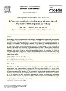
2. Materials and Methods 2.1. Study Area and Sampling. The soils in the experiment were all from Tianshui and Lanzhou, Gansu province, China. They all belonged to loess plateau in China. After sampling, particle size distribution test and analysis were carried out according to the standards of China [34] and operation manual of the laser diffraction apparatus. The soils in this test were from Luoyugou, Tianshui (numbered from L1 to L6), Huanancun, Tianshui (numbered from H1 to H10), and Gaolan, Lanzhou (numbered from G1 to G9). Gaolan samples were obtained from the typical section with 0.4 m of the sample interval. Sample interval in Luoyugou is 150 m in 1 km along the valley. Loess in Huanancun was obtained from backwall of a landslide with 1 m of the sample interval. The sample sections and sample intervals were confirmed by typicality and field condition such as no paleosol layer. All samples were light yellow with
Advances in Materials Science and Engineering macrovoid, root holes, and worm holes. There was plenty of clay concretion in loess in Tianshui, while there was none in loess in Lanzhou. Clay particles had effects on particle size distribution of loess [35]. Sample locations are shown in Figure 1, and the basic properties of loess were presented in Table 1. There are few roots in the loess because organic matter often has a profound effect on the grain size distribution of the sediment samples [36]. 2.2. Testing Apparatus and Experiment. The instrument of laser diffraction apparatus is Microtrac S3500. During the experimental process, lofting canister is repeatedly washed with distilled water. The amount of soil is less and it is discrepant from different areas. The data is collected automatically. The equipment in sieve-pipette method contains standard sieve, electronic scale (precision of 1%), drying oven, 1 L measuring cylinder, sodium hexametaphosphate, densimeter, temperature gauge, stirrer, mortar, and beaker. During the test, sieve classification is carried out on particles whose size is larger than 0.075 mm, and densimeter method is used for the particles with size smaller than 0.075 mm. The test results from the two methods are synthesized as the particle size distribution curve of soil at the end. Laser Diffraction (LD) Techniques. Samples were dried at 105∘ C in drying oven for over 8 hours, and then 2 mm standard sieve was used to get rid of big particles. It was found that all the loess particles in this test were less than 2 mm, and those greater than 2 mm were some plant roots. 30 g loess after 2 mm sieve classification was sealed in hermetic bag. During the experiment, the apparatus of LD was washed by distilled water 5 times at the beginning. Then the samples were divided into 4 parts. Every part was used for testing in sequence. If the four results were quite different, the remaining loess should be mixed and divided and tested again until the error limit was under 0.5% to ensure the reliability. In the sieve-pipette method, samples were well dried at 105∘ C in drying oven for over 8 hours; then about 200 g loess was taken for sieve classification. The sieve classification required even force and one person finishes a whole group work. After the sieve classification, the samples that remained on each standard sieve were weighted. Then 30 g samples of size which was less than 0.075 mm were put into a 1 L measuring cylinder. After addition of some distilled water, 10 mL 4% sodium hexametaphosphate solution was added; then distilled water was poured into the measuring cylinder to 950 mL. The last 50 mL water was added by 50 ml measuring cylinder. The mixture was stirred repeatedly for 1 min, and then decimeter was put in the scheduled time. When storing, the liquid should not be splashed out from the measuring cylinder. At last, the results from sieve classification and densimeter method were synthesized as the final particle distribution curve. 2.3. Brief Introduction of Models. Several PSD functions were proposed to describe the PSD curves. Jaky [37] put forward an exponential function model at the earliest time, which contained a few parameters and was convenient to use but
Advances in Materials Science and Engineering
3
G-5
G-1
G-6 G-2
G-7 G-8
G-3
G-9
G-4 Gaolan
H-1 H-2 H-3 H-4 H-5 H-6 H-7 H-8 H-9 L-6
L-5
L-4
L-3
L-2
L-1
H-10
Luoyugou
Huanancun
Figure 1: Location of sampling.
had poor accuracy. The Shiozawa and Campbell model [38] divided the particle distribution into two parts: sand and silt group and clay group. And scholars such as Buchan et al. [39] found that Shiozawa and Campbell model could not be verified in the clay particle part because of the lack of available data in that range. Lots of other models were proposed such as Fractal model [3], Gompertz model [40], Fredlund model [41], Logarithmic model [4], and exponential model [42]. Every one of them had advantages and disadvantages. Fredlund model was often used to describe the PSD curves of wellgraded and poor-graded soils. Four parameters increased the accuracy. Since Fredlund model was based on continuous function, it had better effect on prediction of soil water characteristic curve. Logarithmic model has a better fitting performance of well-structured soil.
Logarithmic Model. Consider
Jaky Model. Consider
Gompertz Model. Consider
𝐹 (𝑥) = exp {−
𝑥 2 1 [ln ( )] } . 𝑎2 𝑥𝑛
𝐹 (𝑥) = 𝑎 ln 𝑥 + 𝑏.
In the function, 𝑎 and 𝑏 are parameters; 𝑥 is particle size, and its unit is mm. Fredlund Model. Consider 𝐹 (𝑥) =
1 {ln [exp (1) + (𝑎/𝑥)𝑏 ]}
𝑐
{1 − [
7 (3) ln (1 + 𝑑/𝑥) ] }. ln (1 + 𝑑/𝑥𝑚 )
In the function, 𝑎, 𝑏, 𝑐, and 𝑑 are parameters, 𝑥𝑚 = 0.001 mm, and 𝑥 is particle size with mm unit.
𝐹 (𝑥) = 𝑎 + 𝑏 exp {− exp [−𝑐 (𝑥 − 𝑑)]} . (1)
In the function, 𝑥𝑛 = 2 mm, 𝑎 is a parameter, and 𝑥 is particle size with mm unit.
(2)
(4)
In the function, 𝑎, 𝑏, 𝑐, and 𝑑 are parameters and 𝑥 is particle size with mm unit. Jaky model is a one-parameter model which is proposed at an early time with a sigmoid half of a Gaussian lognormal
4
Advances in Materials Science and Engineering Table 1: Physical property indexes of test soil.
distribution. Logarithmic model is a natural logarithm model with two parameters. In Logarithmic model, 𝑎 and 𝑏 are parameters. Gompertz model is closed solution function with four parameters, and it is not sensitive to size interval among test points. The model is a logistic function represented by a closed-form equation with 𝑎, 𝑏, 𝑐, and 𝑑 being shape parameters of the curve. Fredlund model is a four-parameter model which is based on SWCC. In the model, a is the point of inflection of the curve, b is related to its steepest slope, 𝑐 is related to its shape near the fines region, and d is the amount of fine particles. It can fit the particle distribution curve of different soils, and it is a continuous function. Jaky model, Logarithmic model, Gompertz model, and Fredlund model were, respectively, used on particle distribution curves from Luoyugou, Huanancun, and Gaolan. Fitting results of the LD method and the sieve-pipette method on L-3, H-5, and G-7, which are selected by random drawing, are shown in Figures 4 and 5. 2.4. Fitting Techniques. Several approaches have been reported for selection of a suitable model. The simplest approach is to find the best model that minimizes the disparity between measured and predicted data. For example, a model with greater 𝑅2 value may be much more reliable than those with smaller 𝑅2 value. However, it must be known that as the number of parameters increases, the fitting performance generally improves. Statistical terms were used to evaluate the advantages and disadvantages of different models. 𝑅2 was the coefficient of
determination, which was used to estimate the goodness-offit of the model. The range was from 0 to 1. The high 𝑅2 indicates the good fitting performance of the model. The Fvalue was used to estimate the model. The t-value was used to estimate the parameters of the model. The residual sum of squares reflected the deviation between the measured values and estimated values. The mean square was residual sum of squares divided by the number of degrees of freedom. The PSD models considered here required one to four parameters. Therefore, a better approach is to define the good model as the model that fits data well with the least number of parameters when other conditions are the same. Twenty-five groups of loess samples were tested. In order to compare and analyze, this paper showed one group data from Luoyugou (L-3), Huanancun (H-5), and Gaolan (G7), respectively. Logarithmic model, Fredlund model, Jaky model, and Gompertz model were used to fit loess particle size distribution curve in this paper. Other models in references showed poor fitting performance and they were not presented here.
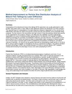
3. Results and Discussion 3.1. Test PSD Results of Loess. The results of the particle size distribution curves from laser diffraction (LD) techniques and the sieve-pipette method on Luoyugou (L-3), Huanancun (H-5), and Gaolan (G-7) were shown in Figures 2 and 3. The sample size of the sieve-pipette method is sixteen, while that of the laser diffraction (LD) techniques is forty-two.
Advances in Materials Science and Engineering
5
100
Percent passing (%)
80
60
40
20
0
1
0.1 0.01 Particle size (mm)
1E − 3
L-3 H-5 G-7
Figure 2: Result of laser diffraction technique.
100
Percent passing (%)
80
60
40
20
0
1
0.01 0.1 Particle size (mm)
1E − 3
L-3 H-5 G-7
Figure 3: Result of sieve-pipette method.
It could be seen from Figures 2 and 3 that the results of the two different methods were relatively similar. Thus, there could be a subtle difference of the soil particle size fraction in Lanzhou and Tianshui. However, the curves of the laser diffraction (LD) techniques were smoother than those of the sieve-pipette method. Sieve-pipette method’s results indicated that the proportion of clay in three different kinds of loess is 11.05%∼13.71%, and the proportions of silt and sand were 67.94%∼68.56% and 17.73%∼27.09%, respectively. In laser diffraction (LD) techniques’ results, the percentage of silt was 72.94%∼78.81%, which was greater than that of sievesettlement method. Meanwhile, the percentage of clay was 2.88%∼4.53%, which was less than the results of sieve-pipette method. Only the percentage of sand was approximate, which was 18.25%∼24.18%.
Comparing sieve-pipette method’s results with laser diffraction (LD) techniques’ results, there was pretty significant difference in clay and silt grain composition, but the disparity of sand grain composition was relatively small. These differences were related to anisotropy of soil particle density and otherness of particle shape. Sieve-pipette method assumed simplex particle density in the soil, but the laser diffraction (LD) techniques were independent of simplex particle density. For laser diffraction (LD) techniques, a single soil particle with irregular shape reflected that its cross section area was bigger than the volume of an equivalent sphere [43]. Therefore, the particle size was magnified, which resulted in less silt proportion in a loess particle distribution curve. Besides that, nonspherical particle had longer setting time than the equivalent sphere in the sieve-pipette method, resulting in a larger clay proportion in a particle size distribution curve. 3.2. Fitting Performance. From Figures 4(a), 4(b), and 4(c), it is observed that Fredlund model and Gompertz model have better fitting performances than the others. The Jaky model curves deviated from the measured points, and Logarithmic model followed. They have poor fitting performances. Gompertz model has relatively good effects, but the particle size of the inflection of the particle distribution curve is 0.05∼ 0.10 mm, with small deviations. However, Fredlund model is almost coincident to measured datum with slight deviation at 0.001∼0.005 mm particle size range. The range of parameter 𝑎 in Jaky model with a typical 95% confidence interval of 0.93 is 4.367∼5.297 (see Table 2). Compared to Jaky model, Logarithmic model has two parameters. Degree of freedom (DF) is 40; the range of parameter 𝑎 is 0.166∼0.210, and its interval is 0.044, which means a small fluctuation. The range of parameter 𝑏 is 106.948∼123.301, and its interval is 16.353 with a larger fluctuation. In Fredlund model, the ranges of parameters 𝑎, 𝑏, 𝑐, and 𝑑 are 0.031∼0.036, 1.879∼2.968, 0.940∼2.723, and −46.323∼52.659, respectively. In Gompertz model, they are −0.132∼−0.084, 1.077∼1.127, 48.374∼51.736, and 0.018∼0.020 with intervals as 0.048, 0.050, 3.362, and 0.002. ̂ 2 , ranging from 0.855 to The four models all have large 𝑅 1.000. Besides Jaky model, the other three models were all significant at the 𝑝 < 0.01 level (Logarithmic: 𝐹 = 462.488; Fredlund: 𝐹 = 92120.82; Gompertz: 𝐹 = 99005.573). The results of the t-tests indicated statistical significance for all the parameters of Gompertz model and Logarithmic model. But the small t-value of parameter 𝑑 in Fredlund model is 0.130, which is not significant. It means that although this model is undergoing the test, its critical parameter 𝑑 may be zero, which may influence the initial form of model. The statistics mean square of Fredlund model is 0.589, which is identical to the phenomenon stating that the fitting and measured data have huge disparity at the 0.001∼0.005 mm particle range. The mean square of Gompertz model is 0.548 which is far below that of Logarithmic model, 225.026. Thus, Gompertz model has better comprehensive effects than Logarithmic model. In sum, Jaky model and Logarithmic model have few parameters and larger degree of freedom, but the mean squares are well above Fredlund model and Gompertz model, which verify the
Advances in Materials Science and Engineering 100
100
80
80 Percent passing (%)
Percent passing (%)
6
60
40
20
0
60
40
20
1
0.1 0.01 Particle size (mm)
Testing data Jaky model Logarithmic model
0
1E − 3
Fredlund model Gompertz model
1
0.1 0.01 Particle size (mm)
Testing data Jaky model Logarithmic model
(a) G-7
1E − 3
Fredlund model Gompertz model
(b) H-5
100
Percent passing (%)
80
60
40
20
0
1
0.1 0.01 Particle size (mm)
Testing data Jaky model Logarithmic model
1E − 3
Fredlund model Gompertz model (c) L-3
Figure 4: Performance of models fitted to LD particle size distributions.
phenomenon stating that fitting curve highly deviated from measured datum in Figure 4. Within the range of 0.001∼0.005 mm particle, comparing Fredlund model and Gompertz model, Fredlund model has a big degree of deviation at range of accumulation curve, which shows poorer fitting performance. Gompertz model has a big degree of deviation at 0.05∼0.10 mm particle range of accumulation curve, and at this range it shows poorer fitting performances. Fredlund model and Gompertz model both have great fitting performance in the ranges of 0.005∼ 0.05 mm and 0.10∼1.0 mm. Thus, for particle size distribution curve of the Gaolan loess sample, when particle size is less than 0.005 mm, Gompertz model has better fitting performance, and when particle size is greater than 0.005 mm, Fredlund model shows greater fitting performance.
Similarly, the range of parameter 𝑎 in Jaky model with a typical 95% confidence interval of 0.939 is 4.170∼5.109 (see Table 3). Compared to Jaky model, the interval of parameter 𝑎 in Logarithmic model has actually a small value, 0.052, and the parameter 𝑏 has indeed a large interval, 17.015. Intervals of parameters 𝑎, 𝑏, 𝑐, and 𝑑 of Fredlund model are 0.003, 0.762, 0.858, and 62.208, respectively, while intervals of parameters 𝑎, 𝑏, 𝑐, and 𝑑 of Gompertz model are 0.024, 0.026, 2.712, and 0.001, respectively (the models were all under the significance level of 5%). Jaky model, Logarithmic model, Fredlund model, and ̂ 2 , ranging from 0.850 to Gompertz model all have large 𝑅 1.000. Besides Jaky model, the other three models were all significant at the 𝑝 < 0.01 level (Logarithmic: 𝐹 = 404.349; Fredlund: 𝐹 = 119670.944; Gompertz: 𝐹 = 122720.519). Thus,
7
100
100
80
80 Percent passing (%)
Percent passing (%)
Advances in Materials Science and Engineering
60
40
40
20
20
0
60
1
0.1 0.01 Particle size (mm)
Testing data Jaky model Logarithmic model
0
1E − 3
Fredlund model Gompertz model
1
0.1 0.01 Particle size (mm)
Testing data Jaky model Logarithmic model
(a) G-7
1E − 3
Fredlund model Gompertz model
(b) H-5
100
Percent passing (%)
80
60
40
20
0
1
0.1 0.01 Particle size (mm)
Testing data Jaky model Logarithmic model
1E − 3
Fredlund model Gompertz model (c) L-3
Figure 5: Performance of models fitted to sieve-pipette particle size distributions.
Jaky model is not suitable for Huanancun loess. The statistics mean square of Jaky model is 279.737, which verifies the phenomenon stating that the curve is highly deviated from measured datum in Figure 5. Similar to Gaolan loess results, the t-tests presented statistical significance under significance level of 1% for all the parameters of Gompertz model and Logarithmic model. But the small t-value of parameter 𝑑 in Fredlund model is 0.240, which is still not significant under significance level of 1%, 5%, and 10%. It means that although this model is undergoing the test, its critical parameter 𝑑 may be zero, which may influence the initial form of model as well. The statistics mean square of Fredlund model is 0.458, which is identical to the phenomenon stating that the fitting and measured data have huge disparity at the 0.001∼
0.005 mm particle range in Figure 5. The mean square of Gompertz model is 0.447, which is far below that of Logarithmic model, 258.786. Accordingly, the Gompertz model has better comprehensive effects in comparison to Logarithmic model. To sum up, Jaky model and Logarithmic model have poorer fitting performance compared to Fredlund model and Gompertz model, which is coincident to the phenomenon stating that fitting curve highly deviated from measured datum in Figure 5. Similarly, as can be seen from the data in Table 4, results of Luoyugou loess samples are the same as those of Gaolan and Huanancun ones. Although Jaky model and Logarithmic model have few fitting parameters and larger degree of freedom, the mean squares are greater than Fredlund model
8
Advances in Materials Science and Engineering Table 2: Fitting parameters of G-7 by laser diffraction technique.
M V a b ̂2 𝑅 𝐹-value 𝑃 value Mean square Degrees of freedom M V a b c d ̂2 𝑅 𝐹-value 𝑃 value Mean square Degrees of freedom
Jaky Value 4.832∗∗ (20.97) —
Value 0.034∗∗ (29.992) 2.424∗∗ (9.016) 1.831∗∗ (4.160) 3.168 (0.130)
Min 4.367 — 0.855 773.289 1.000 266.667 41 Fredlund Min 0.031 1.879 0.940 −46.323 1.000 92120.82 0.000 0.589 38
Max 5.297 —
Max 0.036 2.968 2.723 52.659
Logarithmic Value Min 0.188∗∗ (17.20) 0.166 115.125∗∗ (28.46) 106.948 0.878 462.488 0.000 225.026 40 Gompertz Value Min −0.108∗∗ (−9.141) −0.132 1.102∗∗ (89.647) 1.077 50.055∗∗ (60.283) 48.374 0.019∗∗ (40.111) 0.018 1.000 99005.573 0.000 0.548 38
Max 0.210 123.301
Max −0.084 1.127 51.736 0.020
(Note. ∗∗ Statistically significant at 0.05. Note that significance levels are one-tailed tests if matching a predicted direction and two-tailed tests otherwise. M represents “model”; V represents “value.” The same applies to Tables 3–12.)
Table 3: Fitting parameters of H-5 by laser diffraction technique. M V a b ̂2 𝑅
Jaky Value 4.639∗∗ (19.963) —
𝐹-value 𝑃 value Mean square Degrees of freedom M V a b c d ̂2 𝑅 𝐹-value 𝑃 value Mean square Degrees of freedom
Value 0.040∗∗ (53.339) 2.805∗∗ (14.907) 1.769∗∗ (8.360) 3.689 (0.240)
Min 4.170 — 0.850 744.210 1.000 279.737 41 Fredlund Min 0.039 2.424 1.341 −27.415 1.000 119670.944 0.000 0.458 38
and Gompertz model, which present the phenomenon stating that curves diverge from measured datum weakly in Figure 6. Compared with Fredlund model and Gompertz model, Fredlund model has better fitting performance in 0.001∼ 0.005 mm range of accumulation curve. Fitting performance on 0.05∼0.10 mm of Gompertz model is worse than Fredlund
Max 5.109 —
Value 0.191∗∗ (15.776) 112.659∗∗ (26.785)
Max 0.042 3.186 2.199 34.793
Value −0.041∗∗ (−6.840) 1.037∗∗ (160.344) 48.736∗∗ (72.814) 0.026∗∗ (85.031)
Logarithmic Min 0.116 104.152 0.861 404.349 0.000 258.786 40 Gompertz Min −0.053 1.024 47.380 0.025 1.000 122720.519 0.000 0.447 38
Max 0.168 121.167
Max −0.029 1.050 50.092 0.026
model. These two models both have good fitting results on the ranges of 0.005∼0.05 mm and 0.10∼1.0 mm. Thus, for particle distribution curve of Luoyugou loess samples, when particle size is smaller than 0.005 mm, Gompertz model has good fitting performance, which means great prediction effects. And when particle size is larger than 0.005 mm, Fredlund
Advances in Materials Science and Engineering
9
Table 4: Fitting parameters of L-3 by laser diffraction technique. M V a b ̂2 𝑅 𝐹-value 𝑃 value Mean square Degrees of freedom M V a b c d ̂2 𝑅 𝐹-value 𝑃 value Mean square Degrees of freedom
Jaky Value 4.754∗∗ (18.940) —
Value 0.038∗∗ (46.947) 3.072∗∗ (11.835) 1.691∗∗ (6.584) 2.337 (0.182)
Min 4.246 — 0.833 685.062 1.000 312.119 41 Fredlund Min 0.036 2.546 1.171 −23.692 1.000 84361.639 0.000 0.671 38
model has better fitting results. In conclusion, when choosing the fitting models for particle distribution curve from the LD method of Tianshui and Lanzhou loess samples, the decision should be based on the particle size in loess. If there is plenty of clay in the loess, priority selection should be made to Gompertz model. And if there is little clay, on the contrary, it is better to choose Fredlund model for fitting and prediction. Tables 5–7 provide critical values of particle distribution curve of the sieve-pipette method. Fitting performance can be found in Figures 5(a), 5(b), and 5(c). It is observed that in tables showing the fitting results of Gaolan, Huanancun, ̂ 2 are all approximate to 1, between 0.899 and Luoyugou, 𝑅 and 0.991. Jaky model is not even significant at the 𝑝 < 0.1 level (Gaolan: 𝐹 = 892.648; Huanancun: 𝐹 = 757.463; Luoyugou: 𝐹 = 1199.540). Meanwhile, the statistics mean squares are 88.061, 97.584, and 60.471, respectively, which denote the worst fitting performance. The other three models are all significant at the 𝑝 < 0.001 level, which means that the equations are all valid. However, in perspective of statistics mean squares, the value ranking was followed by Fredlund model, Gompertz model, and Logarithmic model. The mean squares of Fredlund model are 10.494, 11.358, and 11.451, respectively. The mean squares of Gompertz model are 13.272, 12.737, and 17.010, respectively. The mean squares of Logarithmic model are 114.457, 122.522, and 84.141, respectively. Because of the small number of samples, 16, the 𝑡 value is not significant in sieve-pipette method. By the same token, the data points are scattered in the figure. Therefore, the 𝑡 value in sieve-pipette method is elided. As can be seen by comparing LD method and sievepipette method, Fredlund model has better fitting performance than Gompertz model, Logarithmic model, and Jaky
Max 5.261 —
Value 0.190∗∗ (14.906) 113.702∗∗ (21.592)
Max 0.039 3.597 2.212 28.367
Value −0.026∗∗ (−6.405) 1.024∗∗ (233.538) 56.442∗∗ (93.406) 0.024∗∗ (128.52)
Logarithmic Min 0.164 104.745 0.847 374.964 0.000 286.852 40 Gompertz Min −0.034 1.016 55.218 0.024 1.000 197478.102 0.000 0.286 38
Max 0.215 122.659
Max −0.018 1.033 57.666 0.025
model of Malan loess in Lanzhou and Tianshui. But the number of parameters, four, in Fredlund model makes it more difficult to solve equation when predicting SWCC. In the meantime, it makes the model more complex. For this reason, this paper proposes an empirical model with three parameters. Results of this empirical model are shown in Figures 6 and 7 and Tables 8–13. Mathematical expression of the empirical model is shown as follows: 𝐹 (𝑥) =
𝑎 . 𝑏 + exp (−𝑐𝑥)
(5)
In the function, 𝑎, 𝑏, and 𝑐 are parameters and 𝑥 is particle size with mm unit. The empirical model was obtained by the PSD curves of loess in Lanzhou and Tianshui, Gansu, China. Because of the differences in PSD curves of loess, parameters 𝑎, 𝑏, and 𝑐 may be related to 𝐶𝑢 and 𝐶𝑐 of the loess. From Figures 2 and 3, it is obvious that the uniformity coefficient (𝐶𝑢 ) and the coefficient of gradation (𝐶𝑐 ) are different in the loess. Generally, a soil is referred to as well-graded type if 𝐶𝑢 is larger than 4–6 and 𝐶𝑐 is between 1 and 3 [44]. 𝐶𝑢 of L-3, H5, and G-7 is 4.05∼30.90. 𝐶𝑐 of L-3, H-5, and G-7 is 1.05∼1.31. So the loess samples in the study all belong to well-graded soil. Because loess in the study belongs to well-graded soil, the fluctuation range of 𝑎, 𝑏, and 𝑐 is small. 𝐶𝑐 =
𝑑30 2 , 𝑑10 × 𝑑60
𝑑 𝐶𝑢 = 60 . 𝑑10
(6)
Advances in Materials Science and Engineering 100
100
80
80 Percent passing (%)
Percent passing (%)
10
60
40
20
0
60
40
20
1
0.1 0.01 Particle size (mm)
0
1E − 3
Testing data Fitting line
1
0.1 0.01 Particle size (mm)
1E − 3
Testing data Fitting line (a) G-7
(b) H-5
100
Percent passing (%)
80
60
40
20
0
1
0.1 0.01 Particle size (mm)
1E − 3
Testing data Fitting line (c) L-3
Figure 6: Performance of empirical model fitted to LD particle size distributions.
𝐶𝑐 is the coefficient of gradation, 𝐶𝑢 is the uniformity coefficient, and 𝑑10 , 𝑑30 , and 𝑑60 are the diameter through which 10%, 30%, and 60% of the total soil mass is passing, respectively. Figures 6 and 7, respectively, provide the PSD curves that are based on the LD method and sieve-pipette method. By comparing fitting performances of LD method and sievepipette method from Figures 6 and 7, it is shown that the curves of the two methods have roughly the same tendency. Nonetheless, different method results in different inflection points and the dispersion degree of data points on the curves. ̂ 2 of particle size From Tables 8–13, it is shown that 𝑅 distribution curve fitting performance on LD method and ̂ 2 of fitting perforsieve-pipette method are all close to 1. 𝑅 ̂2 mance from LD method is not less than 0.992. Similarly, 𝑅 of fitting performance from sieve-pipette method is not less
than 0.957. The models were all significant at the 𝑝 < 0.01 level. In addition, statistics 𝑡 values of parameters 𝑎, 𝑏, and 𝑐 are all significant under 1% significance level. Consequently, the fitting performance of empirical model is significantly better than those of Logarithmic model and Jaky model. Parameters 𝑎 and 𝑏 of the PSD curve of empirical model in Gaolan, Huanancun, and Luoyugou from the LD method have narrow data ranges, which are less than 0.029 and greater than 0.018. However, parameter 𝑐 has large variations, and the intervals are 20.460, 15.408, and 15.522, respectively. But, likewise, parameters 𝑎 and 𝑏 of the PSD curves of empirical model in Gaolan, Huanancun, and Luoyugou from the sievepipette method have relatively wide data ranges. They are less than 0.195 and they exceed 0.159. The intervals of parameter 𝑐 are 34.517, 42.637, and 32.798. In general, the variations of parameters 𝑎, 𝑏, and 𝑐 in empirical model are far below
11
100
100
80
80 Percent passing (%)
Percent passing (%)
Advances in Materials Science and Engineering
60
40
40
20
20
0
60
1
0.1 0.01 Particle size (mm)
0
1E − 3
1
0.1 0.01 Particle size (mm)
1E − 3
Testing data Fitting line
Testing data Fitting line (a) G-7
(b) H-5
100
Percent passing (%)
80
60
40
20
0
1
0.1 0.01 Particle size (mm)
1E − 3
Testing data Fitting line (c) L-3
Figure 7: Performance of empirical model fitted to sieve-pipette particle size distributions.
those in Fredlund model and Gompertz model. Thus, they are more stable. But the mean square is slightly larger than those in Fredlund model and Gompertz model. Mean squares of the PSD from the LD method are 14.640, 9.276, and 7.251, respectively. And the mean squares of the PSD curve from the sieve-pipette method are 35.102, 49.772, and 49.122, respectively. This reflects in Figure 7 that the fitting curve skews slightly at 0.001∼0.03 mm of particle size range. No matter in the same area or in different areas, parameters 𝑎 and 𝑏 in empirical model do have narrow data ranges, which are less than 0.195. However, parameter 𝑐 has a large variation. The data range is 15.408 to 42.637. In conclusion, for the fitting performance of PSD curves datum for loess in Lanzhou and Tianshui, the empirical model has better applicability and simpler equation form. There are fewer parameters in the equation and the degree
of freedom of the variable is larger, which is good to enter the operation equation and to solve the equation. Different models show significant discrepancy when fitting the data from the LD method and sieve-pipette method. It is related to not only the different test methods but also the size and shape of the particles directly. It is found in research that Fredlund model and empirical model both have good fitting performance on loess PSD curves in Lanzhou and Tianshui. When using the PSD curves to predict the permeability coefficient and SWCC of unsaturated loess, they both show great superiority. The LD method has better test precision, but it has limitations when testing loess particle size distribution. It may overrate the silt part and underrate clay part. In the sieve-pipette method, inaccuracy of setting time estimation and adhesion of clay particles on densimeter glass bulb may
12
Advances in Materials Science and Engineering Table 5: Fitting parameters of G-7 by sieve-pipette method.
M V a b c d ̂2 𝑅 𝐹-value 𝑃 value Mean square Degrees of freedom
Table 8: Fitting parameters of empirical model on G-7 by laser diffraction technique.
Table 9: Fitting parameters of empirical model on H-5 by laser diffraction technique.
Place V a b c ̂2 𝑅 𝐹-value 𝑃 value Mean square Degrees of freedom
Place V a b c ̂2 𝑅 𝐹-value 𝑃 value Mean square Degrees of freedom
Value 0.052∗∗ (7.383) 0.053∗∗ (7.388) 97.500∗∗ (19.263)
Gaolan Min 0.037 0.038 87.270 0.992 5291.200 0.000 14.640 39
Max 0.066 0.067 107.730
Huanancun Value Min 0.043∗∗ (8.172) 0.032 0.043∗∗ (8.178) 0.033 87.709∗∗ (23.047) 80.005 0.995 7870.769 0.000 9.276 39
Max 0.053 0.054 95.413
Advances in Materials Science and Engineering
13
Table 10: Fitting parameters of empirical model on L-3 by laser diffraction technique.
Table 13: Fitting parameters of empirical model on L-3 by sievepipette method.
Place V a b c ̂2 𝑅 𝐹-value 𝑃 value Mean square Degrees of freedom
Place V a b c ̂2 𝑅 𝐹-value 𝑃 value Mean square Degrees of freedom
Luoyugou Value Min 0.039∗∗ (8.787) 0.030 0.040∗∗ (8.791) 0.030 ∗∗ 98.525 (25.701) 90.764 0.996 10390.67 0.000 7.251 39
Max 0.048 0.049 106.286
Table 11: Fitting parameters of empirical model on G-7 by sievepipette method. Place V a b c ̂2 𝑅 𝐹-value 𝑃 value Mean square Degrees of freedom
Gaolan Value Min 0.256∗∗ (6.673) 0.173 0.265∗∗ (6.688) 0.179 62.493∗∗ (7.823) 45.235 0.969 754.680 0.000 35.102 13
Max 0.338 0.338 79.752
Table 12: Fitting parameters of empirical model on H-5 by sievepipette method. Place V a b c ̂2 𝑅 𝐹-value 𝑃 value Mean square Degrees of freedom
Huanancun Value Min 0.192∗∗ (4.932) 0.108 0.202∗∗ (4.958) 0.114 66.794∗∗ (6.769) 45.475 0.961 500.269 0.000 49.772 13
Max 0.276 0.290 88.112
Value 0.249∗∗ (5.757) 0.260∗∗ (5.757) 52.015∗∗ (6.852)
Luoyugou Min 0.155 0.163 35.616 0.957 494.153 0.000 49.122 13
Max 0.342 0.358 68.414
4. Conclusions We conclude the following: (1) Compared to sieve-pipette method, the LD method can collect more data points during testing, so the curve is more smooth. Compared to sieve-pipette method, the LD method overrates the silt part and underrates the clay part. (2) Four models were used to fit the PSD curves of loess in Lanzhou and Tianshui; it was found that Fredlund model had good fitting performance on data obtained by the LD method and sieve-pipette method. So it is suggested that this model be utilized to predict SWCC of unsaturated loess. According to fitting and analysis of testing results, the empirical model is suitable for Malan loess at the same time. This model has typical advantages such as fewer parameters and simple equation form. It could be used to predict SWCC and permeability coefficient of unsaturated loess too. Sensibility of every parameter in each model is discussed during fitting and analysis procedure. Different sensibility will influence the accuracy of fitting performance.
Conflicts of Interest The authors declare that they have no conflicts of interest.
influence the results. Besides that, because fine particles subside very slowly, environmental temperature has significant influence. The aforementioned diversity affects the fitting results for the same model. Comparing Fredlund model and Gompertz model with empirical model, equation form of the empirical model is simplified significantly, and the number of parameters is reduced with mean square root greater than 0.95. Gompertz model is limited when it fits the datum from the sieve-pipette method. In contrast, the empirical model is suitable for the two methods, and the fitting performance is good.
Acknowledgments The authors thank Ms. Wang Juan (Lanzhou University) for useful suggestions. They also thank Mr. Liu Hongwei (Lanzhou University) and Mr. Fu Xianglong (Lanzhou University) for the help in sampling. Financial support for this study was provided by the National Basic Research Program of China (2014CB744701), Key Laboratory of Loess Earthquake Engineering, China Earthquake Administration (KLLEE-17-004), and the National Natural Science Foundation of China (41362014).
14
References [1] L. M. Arya and J. F. Paris, “Physicoempirical model to predict the soil moisture characteristic from particle-size distribution and bulk density data,” Soil Science Society of America Journal, vol. 45, no. 6, pp. 1023–1030, 1981. [2] N. Romano, P. Nasta, G. Severino, and J. W. Hopmans, “Using bimodal lognormal functions to describe soil hydraulic properties,” Soil Science Society of America Journal, vol. 75, no. 2, pp. 468–480, 2011. [3] A. Kravchenko and R. Zhang, “Estimating the soil water retention from particle-size distributions: a fractal approach,” Soil Science, vol. 163, no. 3, pp. 171–179, 1998. [4] J. Zhuang, J. Yan, and T. Miyazaki, “Estimating water retention characteristic from soil particle-size distribution using a nonsimilar media concept,” Soil Science, vol. 166, no. 5, pp. 308–321, 2001. [5] M. D. Fredlund, G. W. Wilson, and D. G. Fredlund, “Use of the grain-size distribution for estimation of the soil-water characteristic curve,” Canadian Geotechnical Journal, vol. 39, no. 5, pp. 1103–1117, 2002. [6] H. Q. Pham and D. G. Fredlund, “Equations for the entire soilwater characteristic curve of a volume change soil,” Canadian Geotechnical Journal, vol. 45, no. 4, pp. 443–453, 2008. [7] S. I. Hwang and S. E. Powers, “Using particle-size distribution models to estimate soil hydraulic properties,” Soil Science Society of America Journal, vol. 67, no. 4, pp. 1103–1112, 2003. [8] C. E. Leong and H. Rahardjo, “Permeability functions for unsaturated soils,” Journal of Geotechnical & Geoenvironmental Engineering, vol. 123, no. 12, pp. 1118–1126, 1997. [9] L. M. Arya, J. L. Heitman, B. B. Thapa, and D. C. Bowman, “Predicting saturated hydraulic conductivity of golf course sands from particle-size distribution,” Soil Science Society of America Journal, vol. 74, no. 1, pp. 33–37, 2010. [10] M. H. Mohammadi, M. Khatar, and M. Vanclooster, “Combining a single hydraulic conductivity measurement with particle size distribution data for estimating the full range partially saturated hydraulic conductivity curve,” Soil Science Society of America Journal, vol. 78, no. 5, pp. 1594–1605, 2014. [11] C. G. Uchrin, “Indirect methods for estimating the hydraulic properties of unsaturated soils,” Soil Science, vol. 157, no. 6, p. 398, 1994. [12] T. Sakaki, M. Komatsu, and M. Takahashi, “Rules-of-thumb for predicting air-entry value of disturbed sands from particle size,” Soil Science Society of America Journal, vol. 78, no. 2, pp. 454– 464, 2014. [13] D. Li, G. Gao, M. Shao, and B. Fu, “Predicting available water of soil from particle-size distribution and bulk density in an oasisdesert transect in northwestern China,” Journal of Hydrology, vol. 538, pp. 539–550, 2016. [14] F. Yang, G.-L. Zhang, F. Yang, and R.-M. Yang, “Pedogenetic interpretations of particle-size distribution curves for an alpine environment,” Geoderma, vol. 282, pp. 9–15, 2016. [15] L. S. Sklar, C. S. Riebe, J. A. Marshall et al., “The problem of predicting the size distribution of sediment supplied by hillslopes to rivers,” Geomorphology, vol. 277, pp. 31–49, 2017. [16] Z. A. Erguler, “A quantitative method of describing grain size distribution of soils and some examples for its applications,” Bulletin of Engineering Geology and the Environment, vol. 75, no. 2, pp. 807–819, 2016. [17] Y. Li, C. Huang, B. Wang et al., “A unified expression for grain size distribution of soils,” Geoderma, vol. 288, pp. 105–119, 2017.
Advances in Materials Science and Engineering [18] J. Thompson, A. M. A. Sattar, B. Gharabaghi, and R. C. Warner, “Event-based total suspended sediment particle size distribution model,” Journal of Hydrology, vol. 536, pp. 236–246, 2016. [19] X. Wei, X. Li, and N. Wei, “Fractal features of soil particle size distribution in layered sediments behind two check dams: Implications for the Loess Plateau, China,” Geomorphology, vol. 266, pp. 133–145, 2016. [20] A. Kumar, A. A. Gokhale, T. Shukla, and D. P. Dobhal, “Hydroclimatic influence on particle size distribution of suspended sediments evacuated from debris-covered Chorabari Glacier, upper Mandakini catchment, central Himalaya,” Geomorphology, vol. 265, pp. 45–67, 2016. [21] B. He, J. P. Han, F. L. Hou et al., “Role of typical soil particle-size distributions on the long-term corrosion behavior of pipeline steel,” Materials & Corrosion, vol. 67, no. 5, pp. 471–483, 2016. [22] V. Wendling, C. Legout, N. Gratiot, H. Michallet, and T. Grangeon, “Dynamics of soil aggregate size in turbulent flow: Respective effect of soil type and suspended concentration,” Catena, vol. 141, pp. 66–72, 2016. [23] W. B. Kunkel, “Magnitude and character of errors produced by shape factors in stokes’ law estimates of particle radius,” Journal of Applied Physics, vol. 19, no. 11, pp. 1056–1058, 1948. [24] J. Clifton, P. Mcdonald, A. Plater, and F. Oldfield, “An investigation into the efficiency of particle size separation using Stokes’ Law,” Earth Surface Processes & Landforms, vol. 24, no. 8, pp. 725–730, 1999. [25] R. B. Bryant, Laser Light Scattering and Geographic Information Systems: Advanced Methods for Soil Particle Size Analysis and Data Display, The University of Arizona. [26] M. Konert and J. Vandenberghe, “Comparison of laser grain size analysis with pipette and sieve analysis: A solution for the underestimation of the clay fraction,” Sedimentology, vol. 44, no. 3, pp. 523–535, 1997. [27] G. Eshel, G. J. Levy, U. Mingelgrin, and M. J. Singer, “Critical evaluation of the use of laser diffraction for particle-size distribution analysis,” Soil Science Society of America Journal, vol. 68, no. 3, pp. 736–743, 2004. [28] F. J. Arriaga, B. Lowery, and M. D. Mays, “A fast method for determining soil particle size distribution using a laser instrument,” Soil Science, vol. 171, no. 9, pp. 663–674, 2006. [29] T. M. Zobeck, “Rapid soil particle size analyses using laser diffraction,” Applied Engineering in Agriculture, vol. 20, no. 5, pp. 633–639, 2004. [30] L. Pieri, M. Bittelli, and P. R. Pisa, “Laser diffraction, transmission electron microscopy and image analysis to evaluate a bimodal Gaussian model for particle size distribution in soils,” Geoderma, vol. 135, pp. 118–132, 2006. [31] S. Hwang, K. P. Lee, D. S. Lee, and S. E. Powers, “Models for estimating soil particle-size distributions,” Soil Science Society of America Journal, vol. 66, no. 4, pp. 1143–1150, 2002. [32] S. I. Hwang, “Effect of texture on the performance of soil particle-size distribution models,” Geoderma, vol. 123, no. 3-4, pp. 363–371, 2004. [33] B. A. Miller and R. J. Schaetzl, “Precision of soil particle size analysis using laser diffractometry,” Soil Science Society of America Journal, vol. 76, no. 5, pp. 1719–1727, 2012. [34] SL-237, Specification of Soil Test, China Water and Power Press, 1999. [35] X. Tan, F. Liu, L. Hu, A. H. Reed, Y. Furukawa, and G. Zhang, “Evaluation of the particle sizes of four clay minerals,” Applied Clay Science, 2016.
Advances in Materials Science and Engineering [36] K. Vasskog, B. C. Kvisvik, and Ø. Paasche, “Effects of hydrogen peroxide treatment on measurements of lake sediment grainsize distribution,” Journal of Paleolimnology, vol. 56, no. 4, pp. 365–381, 2016. [37] J. Jaky, Soil Mechanics, Egyetemi Nyomda, Budapest, Hungary, 1944. [38] S. Shiozawa and G. S. Campbell, “On the calculation of mean particle diameter and standard deviation from sand, silt, and clay fractions,” Soil Science, vol. 152, no. 6, pp. 427–431, 1991. [39] G. D. Buchan, K. S. Grewal, and A. B. Robson, “Improved models of particle-size distribution: an illustration of model comparison techniques,” Soil Science Society of America Journal, vol. 57, no. 4, pp. 901–908, 1993. [40] A. Nemes, J. H. M. W¨osten, A. Lilly, and J. H. Oude Voshaar, “Evaluation of different procedures to interpolate particle-size distributions to achieve compatibility within soil databases,” Geoderma, vol. 90, no. 3-4, pp. 187–202, 1999. [41] M. D. Fredlund, D. G. Fredlund, and G. W. Wilson, “An equation to represent grain-size distribution,” Canadian Geotechnical Journal, vol. 37, no. 4, pp. 817–827, 2000. [42] D. Gim´enez, W. J. Rawls, Y. Pachepsky, and J. P. C. Watt, “Prediction of a pore distribution factor from soil textural and mechanical parameters,” Soil Science, vol. 166, no. 2, pp. 79–88, 2001. [43] M. Jonasz, “Nonsphericity of suspended marine particles and its influence on light scattering,” Limnology and Oceanography, vol. 32, no. 5, pp. 1059–1065, 1987. [44] American Society for Testing and Materials, Annual Book of ASTM Standards, sec. 4, vol. 04.08, West Conshohocken, PA, USA, 2006.