DESY 18-043
Five-Particle Phase-Space Integrals in QCD
arXiv:1803.09084v1 [hep-ph] 24 Mar 2018
O. G ITULIAR
[email protected] V. M AGERYA
[email protected] A. P IKELNER 1
[email protected] II. Institut für Theoretische Physik, Universität Hamburg, Luruper Chaussee 149, D-22761 Hamburg, Germany March 28, 2018
We present analytical expressions for the 31 five-particle phase-space master integrals in massless QCD as an ǫ-series with coefficients being multiple zeta values of weight up to 12. In addition, we provide computer code for the Monte-Carlo integration in higher dimensions, based on the RAMBO algorithm, that has been used to numerically cross-check the obtained results in 4, 6, and 8 dimensions.
1. INTRODUCTION Nowadays, perturbative calculations play the key role in describing data from highenergy particle colliders, such as the LHC, as well as in improving the precision of numerical parameters in Standard Model and other models. It is clear now that higher-order calculations will play an even more crucial role in processing data from future high-luminosity colliders, like the FCC or the ILC, where theoretical errors will dominate over experimental statistical errors. These arguments motivate us to make one step forward beyond available fully- inclusive phase-space integrals for a four-particle decay [GGH04] and calculate a set of yet unknown integrals that corresponds to a five-particle decay of a color-neutral off-shell particle in Quantum Chromodynamics. These results, among others, are necessary ingredients in calculating various exclusive quantities with the method of differential equations where they are 1
On leave of absence from Joint Institute for Nuclear Research, 141980 Dubna, Russia.
needed to determine integration constants, as for example discussed in [Git16, GM15] for the three-loop time-like splitting functions [AMV12]. In this paper, we focus on the calculation of master integrals that can be used to express any other integral of the corresponding topology provided a set of integrationby-parts rules (IBP) [CT81] is known. Our approach is based on techniques for solving dimensional recurrence relations (DRR) [Tar96] described in [LM17a, LM17b]. In particular, we use DREAM package [LM17a] to obtain numerical results for desired integrals with 2000-digit precision and restore analytical form in terms of multiple zeta values (MZV) [Fur03, BBV10, LM16] up to weight 12 using the PSLQ method [FBA99] as implemented in Mathematica. We also present a Monte-Carlo code, based on the RAMBO algorithm [KSE86], for numerical integration of the phase-space integrals in arbitrary (integer) number of dimensions that has been used to check consistency of the obtained results. This paper is organized as following. In Section 2 we introduce our notation and describe our calculational method in more details. In Section 3 we provide complete results for four-particle integrals and discuss numerical cross-checks using MonteCarlo integration. In Section 4 we make final remarks. In Appendix A we provide the complete list of master integrals. Additionally we provide auxiliary files on arXiv2 containing the complete master integrals with MZV weight up to 12 as well as the Monte-Carlo integration routines with the corresponding results.
2. THE METHOD We start by identifying a set of five-particle phase-space master integrals by constructing auxiliary topologies containing the four-loop massless propagators from [BC10], taking all physical five-particle cuts of those, and performing the Laportastyle IBP reduction [Lap00, Lap17] implemented in FIRE5 [Smi15]. This gives us 31 master integrals listed in Table 1 with up to 6 unique propagators each. Our notation is Z 1 F i = S Γ dPS5 ( i) , (1) D 1 . . . D (ni) where D (ji) are propagators that take the form of invariant scalar products ¡ ¢2 s kl...q = p k + p l + · · · + p q ,
dPS5 is a five-particle phase-space element in D dimensions à ! ´ N Y ¡ ¢ (D ) ³ D + 2 dPSN = d pi δ pi δ q − p1 − . . . − p N , i=1
2
https://arxiv.org
2
(2)
(3)
F1
F2 : 12 14 23 34
F3 : 01 05
F4 : 12 13 02 03
F5 : 12 34 02 03
F6 : 12 13 02 04 45 35
F7 : 123 124
F8 : 13 14 123 124
F9 : 12 23 023 012
F10 : 01 123
F11 : 01 123 014 05
F12 : 12 023 05
F13 : 12 13 124 05 02
F14 : 02 12 023 05
F15 : 12 13 124 134 02 03
F16 : 12 34 02 03 124 134
F17 : 12 34 013
F18 : 12 13 25 124 05 04
F19 : 12 13 25 124 013 05
F20 : 12 13 124 134 35 25
F21 : 12 13 24 012 05
F22 : 12 13 24 012 45 05
F23 : 12 13 25 45 134 012
F24 : 12 13 45 134 05 03
F25 : 12 13 45 134 012 05
F26 : 012 123
F27 : 12 01 123 013
F28 : 123 012 05 01
F29 : 12 123 25 013 05 01
F30 : 12 13 034 134 05 03
F31 : 12 13 034 134 05 04
Table 1: Cut diagrams for five-particle phase-space master integrals in QCD. Dashed lines represent cut propagators and carry final-state momenta p 1 , . . ., p 5 . Labels represent propagators, so that "123" corresponds to p 1 + p 2 + p 3 and "012" to q − p 1 − p 2 (where q is the initial-state momentum, i.e., q = p 1 + · · · + p 5 ). 3
and S Γ is a common normalization factor chosen for convenience to be ¡
SΓ = q
¢ 2 5−2D
¢4 µ ¶ µ ¶ 2π D D Γ −1 Γ 3 −3 . 2 2 π2D
¡
(4)
With this normalization and knowing the volume of the complete N -particle phase space3 Z
¢N ¡ D Γ D2 − 1 ¢ D2 ( N −1)−N π 2 ( N −1) dPS N = q ¡ ¢ N −1 ³ ¡ D ¢¡ ¢´ ³ ¡ ¢ ´ 2π Γ 2 − 1 N − 1 Γ D2 − 1 N ¡
2
(5)
we can already fix the value of F1 as
F1 = S Γ
Z
¡ ¢6 ¡ ¢ Γ D2 − 1 Γ 3 D2 − 3 dPS5 = ¡ D ¢ ¡ ¢. Γ 4 2 − 4 Γ 5 D2 − 5
(6)
Next, with the help of LiteRed [Lee14] and FIRE5 [Smi15] we derive a set of lowering dimensional recurrence relations which express master integrals in D + 2 dimensions in terms of master integrals in D dimensions:
F i (D + 2) = M i j (D ) F j (D ).
(7)
In our case M can be shuffled into triangular form, with each F i only depending on itself and master integrals from lower sectors S i : X M ik (D )F k (D ) (8) F i (D + 2) = M ii (D ) F i (D ) + k∈S i
and the general solution being
F i ( D ) = ω i ( D ) H i ( D ) + R i ( D ),
(9)
where H i is a homogeneous solution of eq. (8), R i is a partial solution that can be constructed numerically with DREAM [LM17a] provided F1 is known, and ω i (D ) is an arbitrary periodic function that needs to be determined from separate considerations. We argue that all ω i>1 are zero. To see this, first let us look at the asymptotic behavior of F i at large D . Rewriting eq. (1) as an integral over invariants s i j gives
F i = SΓ 3
Ã
N −1 Y k=1
ΩD − k
!ZÃ
Y
l 1 are growing exponentially faster than F i (D ), which can only happen if the corresponding periodic functions ω i (D ) are zero.
Thus, to find F i we only need to find R i , the inhomogeneous solutions to eq. (8). We compute them as a series in ǫ = (4 − D )/2 using DREAM with 2000-digit accuracy and then restore the analytical form of the series coefficients in terms of MZVs using PSLQ method [FBA99]. In this way we obtain the analytical result for all master integrals up to MZVs of weight 12 using the corresponding bases from [Fur03] and the SummerTime package [LM16] for their numerical evaluation. Corresponding expressions are presented in Appendix A as well as in the auxiliary files on arXiv.
5
3. CROSSCHECKS
3.1. F OUR -PARTICLE I NTEGRALS As the first consistency check of our method we reproduce results for four- particle phase-space integrals reported in [GGH04]. We perform all the steps described in Section 2. Generating the IBP rules with the help of LiteRed and then proceeding with DREAM we obtain the final result with 2000-digit accuracy and MZVs up to weight 12. The series reconstructed with PSLQ (using the original notation, and omitting S Γ and q2 factors) are: µ µ ¶ ¶ 61 2 2 R 6 = −1 + ζ2 + ǫ − 12 + 5ζ2 + 9ζ3 + ǫ − 91 + 27ζ2 + 45ζ3 + ζ2 (16) 5 µ ¶ 2 3 + ǫ − 558 + 161ζ2 + 197ζ3 + 61ζ2 − 80ζ3 ζ2 + 207ζ5 µ ¶ 1157 2 288 3 + ǫ4 − 3025 + 939ζ2 + 897ζ3 + ζ2 − 400ζ3ζ2 + 1035ζ5 + ζ2 − 153ζ23 , 5 5 ¶ µ µ ¶ 5 40ζ2 126ζ3 272 3 2 2 2 R 8,a = 4 − 2 − + 14ζ2 + ǫ 1008ζ2ζ3 − 1086ζ5 + ǫ − ζ + 1602ζ3 , (17) ǫ 7 2 ǫ ǫ ¶ µ µ ¶ 17ζ2 44ζ3 183 2 3 19088 3 2 2 − R 8,b = 4 − − ζ + ǫ 376ζ2 ζ3 − 790ζ5 + ǫ − ζ + 698ζ3 . (18) ǫ 5 2 105 2 4ǫ 2ǫ2
3.2. N UMERICAL V ERIFICATION As another cross-check we have calculated the leading terms of the ǫ-expansion of F i numerically using the direct way: through Monte-Carlo integration of eq. (1) over the phase-space. While such a technique can not be easily applied to divergent integrals, we can sidestep such an issue by noting that our master integrals only suffer from IR divergences that disappear already at D = 6. In this way we can check several leading terms of the expansion at D = 4 − 2ǫ by calculating the corresponding integrals in D ≥ 6 since both are connected by dimensional recurrence relations. To calculate a finite integral of the form eq. (1) we choose a uniform mapping from a hypercube into momentum coordinates using an algorithm similar to RAMBO [KSE86] but extended into arbitrary D . Then we calculate the integrand from scalar products of the momenta, and finally we integrate over the hypercube using the Vegas [Lep78] implementation from C UBA [Hah05]. Note that although the integrals we are calculating are finite, the integrands are not. Exposing an integration algorithm like Vegas to such infinities may lead to unpredictable behaviour, so as a precaution we choose to regulate these infinities by adding a small parameter α to the denominator of the integrand, and then to
6
i D =4 2 3 4 5 6 7 8 9 10 11 12 13 14 15 16 17 18 19 20 21 22 23 24 25 26 27 28 29 30 31
– 3.7823(4) – – – 46.46(4) – – 10.436(2) 228.8(1) – – – – – – – – – – – – – – 25.563(6) – 143.9(1) – – –
Numerical results D=6 D=8 1708(2)00 3.1704(2) 1504.7(8) 1007.4(5) 6191(5)00 18.533(2) 2031(2)0 4313(3) 7.1508(5) 62.67(1) 157.34(4) 13729(8) 268.46(8) 6322(6)0 4414(3)0 1243.4(7) 3002(2)00 4982(4)00 2360(2)000 6312(5)0 8402(7)00 1443(1)000 1391(1)00 3347(3)00 15.376(1) 697.3(3) 52.855(7) 4409(3)0 6327(6)0 8955(8)0
4699(1)0 3.0221(1) 725.3(1) 580.80(9) 14496(6)0 15.205(1) 5357(2) 2406.7(4) 6.5093(3) 47.663(4) 102.26(1) 4000(1) 172.80(2) 16048(5) 12952(4) 709.6(1) 5899(3)0 10637(4)0 5777(2)00 20642(5) 24407(8)0 4556(1)00 3997(1)0 8526(3)0 13.6042(7) 397.84(6) 42.917(3) 13702(3) 16181(5) 19055(8)
D=4 – 3.7823736 – – – 46.435253 – – 10.435253 229.11836 – – – – – – – – – – – – – – 25.564747 – 143.97886 – – –
Analytic results D=6 D=8 171085.62 3.1704486 1504.4507 1007.5235 619633.25 18.532303 20297.189 4312.8823 7.1507477 62.667046 157.33521 13732.166 268.45969 63316.356 44117.898 1243.1369 300402.99 498329.79 2362594.9 63147.876 840453.94 1443198.3 139263.92 335128.10 15.376404 697.18948 52.853837 44117.898 63316.356 89611.062
47000.531 3.0221118 725.26806 580.76347 144975.32 15.205538 5355.3611 2406.7943 6.5092878 47.663194 102.26408 4000.2779 172.79805 16049.857 12951.443 709.52840 58965.517 106357.81 577686.64 20642.071 244075.75 455543.43 39966.878 85254.217 13.604247 397.83514 42.917424 13700.597 16178.566 19051.115
Table 2: Numerical results for the ratio F i /F1 with the corresponding uncertainties (standard deviations) indicated in the parenthesis. Missing entries correspond to divergent integrals. calculate the integral with progressively smaller values of α (from 2−30 to 2−100 ), checking if convergence was reached afterwards. The results of this method are summarized in Table 2, and show good agreement between numerical and analytic results. Our integration program is written in C using the GNU Scientific Library [Gou09] and C UBA. Its source code can be found
7
at https://hg.tx97.net/rambo , and also in the auxiliary files on arXiv. With a requested accuracy of 0.1% the complete integration takes less than two days on a 12-core machine, with each integration taking between a minute and two hours.
4. CONCLUSIONS In this paper we present analytical expressions for five-particle phase-space integrals expressed in terms of multiple zeta values up to weight 12. The results are calculated using dimensional recurrence relation method with a 2000-digit accuracy using the DREAM package. We also present computer code for the numerical integration of phase-space integrals in a higher-number of dimensions that has been used to cross-check the obtained results with an accuracy of 0.1%. The approach presented here shows excellent performance for calculating single-scale integrals without ultraviolet divergences and can be easily applied to other problems of this kind.
5. ACKNOWLEDGMENTS We are thankful to Sven Moch for numerous discussions and helpful suggestions concerning this work, and for proofreading this paper. We were pleased to use Axodraw2 [CV16] to draw diagrams for this paper. This work was supported in part by the German Research Foundation DFG through the Collaborative Research Centre No. SFB 676 Particles, Strings and the Early Universe: the Structure of Matter and Space-Time.
A. RESULTS The main results of our work are listed below. For brevity, we truncate them up to MZVs of weight 6. Complete results with weight up to 12 are available in auxiliary files on arXiv.
µ µ ¶ ¶ 53 13 689 13 1 2 15961 3 436013 +ǫ +ǫ − ζ2 + ǫ − ζ2 − ζ3 (19) F1 = 72 288 10368 72 41472 288 18 µ ¶ µ 207493 689 17 2 5668169 5 2206279853 4 96102601 +ǫ − ζ2 − ζ3 + ζ2 + ǫ − ζ2 1492992 10368 72 240 5971968 41472 µ ¶ 207493 901 2 169 65 1249333813 6 437728233961 − ζ3 + ζ2 + ζ3 ζ2 − ζ5 + ǫ − ζ2 2592 960 18 6 214990848 1492992
8
¶ 271337 2 8957 3445 4007 3 169 2 5668169 ζ3 + ζ + ζ3 ζ2 − ζ5 − ζ + ζ − 10368 34560 2 72 24 5040 2 9 3 ¶ ¶ µ µ 10 1 512 55 1 160 130 490 715 F2 = 5 − 4 + 3 − ζ2 + 2 − + ζ2 − ζ3 3 3 3 3 3 3ǫ 3ǫ ǫ ǫ µ ¶ 4390 6370 2816 8192 275 2 1 1450 2080 2 + − ζ2 + ζ3 + 25ζ2 − + ζ2 − ζ3 − ζ ǫ 3 3 3 3 3 3 2 2 µ 6656 25088 36608 13090 18850 + ζ3 ζ2 − 2504ζ5 + ǫ − ζ2 + ζ3 + 400ζ22 − ζ3 ζ2 3 3 3 3 3 ¶ 3 13136 2 + 13772ζ5 − 211ζ2 + ζ3 3 ¶ µ µ ¶ 7 ζ2 111 2 4231 227 219 7 F3 = − + ǫ − ζ2 − 6ζ3 + ǫ2 − ζ2 − 42ζ3 − ζ2 8 2 16 2 32 8 10 µ µ ¶ 3999 499 777 2 3 65347 4 887695 +ǫ − ζ2 − ζ3 − ζ + 86ζ3 ζ2 − 237ζ5 + ǫ 64 16 2 10 2 128 ¶ 64219 6303 5967 2 1827 3 2 − ζ2 − ζ3 − ζ + 602ζ3 ζ2 − 1659ζ5 − ζ + 204ζ3 32 4 16 2 20 2 µ ¶ µ ¶ ζ2 1 ζ2 39 1 3 13 267 2 267 2 F4 = − 3 + 2 − 13ζ3 + ζ2 + ζ3 − ζ2 + 4ζ2 + ζ3 + ζ ǫ ǫ 2 ǫ 2 2 10 2 20 2 µ 801 2 191 1129 16547 3 1129 + 191ζ3ζ2 − ζ5 + ǫ 10ζ2 + 52ζ3 + ζ2 − ζ3 ζ2 + ζ5 − ζ 2 20 2 4 70 2 ¶ 2 + 487ζ3
7ζ22
µ ¶ 1 7 2 7 435 647 3 F5 = 2 + − ζ2 − 18ζ3 ζ2 + 87ζ5 − ζ22 + 45ζ3 ζ2 − ζ5 + ζ2 − 108ζ23 ǫ 2 10 2 5 5ǫ ¶ ¶ µ µ 35 1 1697 1687 3236 19 1 278 191 F6 = − 5 − 4 + 3 − − ζ2 + 2 + ζ2 − ζ3 3 3 3 18 9 9ǫ 6ǫ ǫ ǫ µ ¶ 7793 10450 31259 67705 1 2386 4927 2 + − + ζ2 + ζ3 − ζ2 + − ζ2 + 4296ζ3 ǫ 3 9 3 18 3 9 µ 209681 2 14708 28148 117869 317353 + ζ2 + ζ3 ζ2 − ζ5 + ǫ − + ζ2 − 31444ζ3 180 3 3 3 9 ¶ 66809 2 101858 84602 357871 3 96472 2 − ζ − ζ3 ζ2 + ζ5 − ζ + ζ3 45 2 9 3 126 2 9 µ µ ¶ ¶ 351 163 36 2 2 F7 = −1 + ζ2 + ǫ − 17 + 10ζ2 + 9ζ3 + ǫ − + ζ2 + 90ζ3 + ζ 2 2 5 2 µ µ ¶ 5709 2495 80649 1337 3 2 4 +ǫ − + ζ2 + ζ3 + 72ζ2 − 151ζ3 ζ2 + 207ζ5 + ǫ − 4 4 2 8 ¶ 35823 18035 4881 2 387 3 2 + ζ2 + ζ3 + ζ − 1510ζ3 ζ2 + 2070ζ5 − ζ − 387ζ3 8 4 10 2 10 2
9
(20)
(21)
(22)
(23) (24)
(25)
µ ¶ ¶ µ µ 1 127 1 145 392 11 1 49 49 539 1 + ζ2 − ζ3 + − ζ2 F8 = 5 − 4 + 3 8 − ζ2 + 2 − 6 2 12 3 ǫ 2 3 2ǫ 4ǫ ǫ ǫ ¶ 439 2401 823 2 2032 9053 2 1829 1397 + ζ3 − ζ2 − + ζ2 − ζ3 + ζ + ζ3 ζ2 6 60 2 6 3 120 2 3 µ 6223 3292 2 20119 26191 2381 1309 7105 − ζ5 + ǫ − ζ2 + ζ3 − ζ2 − ζ3 ζ2 + ζ5 3 2 6 3 15 6 6 ¶ 48983 3 2 + ζ + 1397ζ3 1260 2 µ ¶ µ ¶ ζ2 1 ζ2 21 1 3 7 17 2 17 2 F9 = − 3 + 2 − 7ζ3 + ζ2 + ζ3 + ζ2 + 4ζ2 + ζ3 − ζ + 131ζ3ζ2 ǫ 2 2 10 2 20 2 ǫ ǫ 2 ¶ µ 51 2 131 127 7677 3 127 − ζ5 + ǫ 10ζ2 + 28ζ3 − ζ2 − ζ3 ζ2 + ζ5 + ζ2 + 328ζ23 2 20 2 4 70 ¶ µ µ ¶ 3 903 47 15 165 171 2 2 F10 = ζ2 − + ǫ − + ζ2 + 11ζ3 + ǫ − + 58ζ2 + ζ3 + ζ 2 2 2 4 2 10 2 µ µ ¶ 13795 951 184655 1003 513 2 739 3 4 +ǫ − + ζ2 + ζ3 + ζ2 − 159ζ3ζ2 + ζ5 + ǫ − 8 2 2 4 2 16 ¶ 14539 6507 2 2385 11085 1293 3 2 + ζ2 + 3092ζ3 + ζ − ζ3 ζ2 + ζ5 + ζ − 374ζ3 4 10 2 2 4 14 2 µ ¶ 48 3 2 F11 = 10ζ2 ζ3 − 16ζ5 + ǫ − 5ζ3 ζ2 + 8ζ5 − ζ2 + 43ζ3 35 µ µ ¶ 2ζ3 37 2 481 2 2 F12 = − − 13ζ3 − ζ2 + ǫ − 76ζ3 − ζ + 30ζ3 ζ2 − 115ζ5 + ǫ − 422ζ3 ǫ 5 10 2 ¶ 1406 2 1495 158 3 2 − ζ + 195ζ3 ζ2 − ζ5 − ζ + 112ζ3 5 2 2 7 2 ¶ µ µ µ ¶ 1 1 49 11 86 1 145 473 11 1 8 ζ2 F13 = 5 − + 2 − + − ζ2 + ζ3 + + 8ζ2 − ζ3 + 3 4 6 4 3 ǫ 6 3 6ǫ 12ǫ ǫ 3 2 ǫ ¶ µ 439 49 1376 57761 2 5251 2 1309 + ζ2 − − ζ2 + ζ3 − ζ2 − 466ζ3ζ2 + 1794ζ5 + ǫ 60 6 2 3 120 6 ¶ 145 4214 21004 2 1349771 3 2 + ζ2 − ζ3 + ζ + 2563ζ3 ζ2 + −9867ζ5 + ζ − 1372ζ3 2 3 15 2 1260 2 ¶ µ 8ζ22 28 2 164 2 6248 3 2 F14 = − − ζ2 − 48ζ5 + ǫ − ζ − 168ζ5 − ζ + 6ζ3 5ǫ 5 5 2 105 2 µ ¶ µ ¶ µ 1 311 73 281 689 445 563 1 41 1 1 F15 = 6 + − ζ2 + − ζ2 − ζ3 3 + 2 − + 4 − 5 36 18 18 36 9 9 6ǫ 36 ǫ ǫ ǫ ǫ ¶ µ 1 2024 7759 5273 907 7103 2 13933 10553 2 + ζ2 − ζ3 − ζ2 + − ζ2 + ζ3 + ζ 36 18 180 ǫ 9 18 18 120 2 ¶ 1489 3257 6158 12437 22193 28621 2 14065 + ζ3 ζ2 − ζ5 − + ζ2 − ζ3 + ζ + ζ3 ζ2 3 3 9 9 9 120 2 18
10
(26)
(27)
(28)
(29) (30)
(31)
(32) (33)
3631 134489 3 ζ5 − ζ2 + 1189ζ23 6 420 µ ¶ ¶ µ µ 1 209 157 289 1 7 1 185 65 76 1 − ζ2 + 3 − ζ2 − ζ3 + 2 − (34) + 4 − F16 = 6 + 5 36 18 12 9 3 6ǫ 12ǫ ǫ ǫ 18 ǫ ¶ µ 3563 215 10927 2 14431 7041 2 1 239 2123 + ζ2 − ζ3 − ζ2 + − ζ2 + ζ3 − ζ 36 2 180 ǫ 9 18 18 40 2 ¶ 5623 170591 2 8963 857 688 − ζ2 − ζ3 + ζ + ζ3 ζ2 + 463ζ3ζ2 − 1411ζ5 + 9 3 9 120 2 6 8349 134141 3 4169 2 − ζ5 − ζ + ζ 2 180 2 ¶ 3 3 µ µ 4ζ3 1 1008 2 84 2 2 F17 = 2 + 10ζ3 + ζ2 + 48ζ3 + 42ζ2 − 52ζ3 ζ2 + 280ζ5 + ǫ 236ζ3 + ζ (35) ǫ ǫ 5 5 2 ¶ 588 3 2 − 130ζ3ζ2 + 700ζ5 + ζ − 160ζ3 5 2 µ µ µ ¶ ¶ 1937 71 1 1 205 323 5 1 223 1 4019 − + + F18 = − + ζ + − ζ + ζ + (36) 2 2 3 36 18 24 3 9 12ǫ6 8ǫ5 ǫ4 12 ǫ3 ǫ2 ¶ µ 1 3047 26681 443 46931 2 5473 2 3137 − ζ2 − ζ3 + ζ2 + + ζ2 − 1465ζ3 − ζ − 12 18 360 ǫ 2 18 144 2 ¶ 9113 27953 39460 54149 60682 33061 2 − ζ3 ζ2 + ζ5 + − ζ2 + ζ3 − ζ 9 9 9 9 9 24 2 15967 12313867 3 6415 ζ3 ζ2 − ζ5 + ζ2 − 2302ζ23 + 18 18 7560 ¶ ¶ µ µ µ 1 1 371 1 9157 19 1 64 173 1895 2767 F19 = − 6 + 5 + 4 + ζ2 + 3 − − ζ2 + ζ3 + 2 (37) 36 18 72 9 18 4ǫ 8ǫ ǫ 9 ǫ ǫ ¶ µ 1 5798 24635 1451 3439 32357 2 7103 17023 2 − − ζ2 − ζ3 + ζ2 + + ζ2 − ζ3 − ζ 18 18 360 ǫ 3 18 18 720 2 ¶ 4127 18073 111845 120679 49330 3664 2 50743 − ζ3 ζ2 + ζ5 + − ζ2 + ζ3 − ζ + ζ3 ζ2 9 9 18 18 9 5 2 18 53357 10750309 3 7078 2 − ζ5 + ζ2 − ζ 18 7560 9 ¶3 µ ¶ µ 1 1595 85 1 775 325 985 1705 20 − ζ2 + 3 − − ζ2 − ζ3 (38) F20 = 6 + 5 + 4 − 12 9 18 9 9 9ǫ 6ǫ ǫ ǫ ¶ µ µ 1 6445 88 2 3815 4775 1 26455 8935 + 2 − ζ2 + ζ2 − ζ3 + ζ2 + ζ3 − 3635 + 9 9 4 6 ǫ 18 6 ǫ ¶ 743 2 23485 7535 121310 80005 7415 9299 2 − ζ2 + ζ3 ζ2 − ζ5 + − ζ2 + ζ3 + ζ 36 9 3 9 9 9 24 2 189155 26065 134581 3 54985 2 + ζ3 ζ2 − ζ5 + ζ2 + ζ3 18 2 126 9 µ µ µ ¶ ¶ 3 49 33 11 1 1 158 1 145 1 − ζ2 + ζ3 + + 24ζ2 (39) F21 = 5 − 4 + 3 8 + ζ2 + 2 − 2ǫ 4ǫ ǫ 2 ǫ 2 4 3 ǫ 2 +
11
¶ 439 147 1205 2 2528 13255 2 2326 5614 869 ζ3 + ζ2 − − ζ2 + ζ3 − ζ2 − ζ3 ζ2 + ζ5 − 3 12 2 2 3 24 3 3 µ 7742 4820 2 12793 30877 565729 3 1309 435 +ǫ + ζ2 − ζ3 + ζ2 + ζ3 ζ2 − ζ5 + ζ 2 2 3 3 3 3 1260 2 ¶ 5108 2 − ζ 3 3 µ µ ¶ ¶ 23 2521 127 1 1777 190 692 55 1 F22 = 6 + 5 + 4 − − ζ2 + 3 − ζ2 − ζ3 36 3 9 3 3 9ǫ 9ǫ ǫ ǫ ¶ µ µ 1 32441 7993 11117 11419 1 400 11507 2 + 2 − + ζ2 − ζ3 − ζ + − ζ2 18 12 3 90 2 ǫ 18 3 ǫ ¶ 6109 2 28472 15326 99143 50243 33388 12061 + ζ3 + ζ2 + ζ3 ζ2 − ζ5 − + ζ2 − ζ3 3 18 9 3 18 6 3 16091 2 13690 5165 539759 3 61504 2 − ζ2 + ζ3 ζ2 + ζ5 − ζ + ζ3 360 9 3 630 2 9 ¶ ¶ µ µ 1 3565 1345 2255 115 1 2645 1345 115 − ζ2 + 3 + ζ2 − ζ3 − + − F23 = 36 18 18 36 9 18ǫ6 36ǫ5 ǫ4 ǫ ¶ µ µ 1 16445 41695 1 2255 1235 2 5750 30935 + ζ2 + ζ3 + ζ + − ζ2 + 2 − 9 36 18 12 2 ǫ 9 18 ǫ ¶ 51865 1235 2 26705 9910 50945 67250 69905 ζ3 − ζ2 + ζ3 ζ2 − ζ5 − + ζ2 − ζ3 + 18 24 9 3 9 9 9 28405 2 26705 4955 280151 3 45385 2 − ζ2 − ζ3 ζ2 + ζ5 − ζ + ζ3 24 18µ 3 ¶ 252 2 9 ¶ µ µ 1 370 89 568 1 179 67 2197 17 1 1 − ζ2 + 3 − ζ2 − ζ3 + 2 − F24 = 6 + 5 + 4 − 12 9 9 3 9 18 3ǫ 9ǫ ǫ ǫ ǫ ¶ µ 9253 1 669 5840 466 9659 2 14671 6923 2 + ζ2 − ζ3 − ζ2 + − ζ2 + ζ3 − ζ 36 3 90 ǫ 2 9 9 90 2 ¶ 2836 16739 3441 33956 628781 2 18284 + ζ3 ζ2 − 2610ζ5 − + ζ2 − ζ3 + ζ + ζ3 ζ2 3 18 2 9 360 2 9 746701 3 7664 2 ζ2 + ζ − 3109ζ5 − 630 3 3¶ ¶ µ µ 14 1 2182 187 1159 1 1 358 203 F25 = 5 − 4 + 3 − − ζ2 + 2 + ζ2 − ζ3 9 9 9 6 9 9ǫ ǫ ǫ ǫ µ ¶ 10072 3946 40714 25759 1 5333 6451 2 + ζ2 + ζ3 − ζ2 + − ζ2 + 1442ζ3 + − ǫ 9 9 18 45 9 9 µ 48637 2 13613 154768 122299 + ζ2 + ζ3 ζ2 − 3923ζ5 + ǫ − + ζ2 − 10793ζ3 90 9 9 9 ¶ 19313 2 21757 22801 3443939 3 25937 2 − ζ − ζ3 ζ2 + ζ5 − ζ + ζ3 45 2 6 2 1890 2 9
12
(40)
(41)
(42)
(43)
µ ¶ µ µ ¶ 111 2 165 3 4855 2 ζ2 − 90ζ3 − ζ +ǫ F26 = 2 − ζ2 + ǫ 32 − 9ζ2 − 10ζ3 + ǫ 313 − 2 10 2 2 µ ¶ 999 2 2905 65815 45421 − ζ2 − 669ζ3 − ζ2 + 164ζ3 ζ2 − 268ζ5 + ǫ4 − ζ2 4 10 4 8 ¶ 12339 2 1383 3 9533 2 − ζ3 − ζ + 1476ζ3ζ2 − 2412ζ5 + ζ + 430ζ3 2 20 2 70 2 µ ¶ µ 2ζ3 1 52 2 26 2 78 F27 = 2 + − ζ3 + ζ2 − 3ζ3 − ζ2 − 8ζ3 ζ2 + 178ζ5 + ǫ − 8ζ3 − ζ22 ǫ 5 5 5 ǫ ¶ 5342 3 + 4ζ3 ζ2 − 89ζ5 + ζ + 10ζ23 35 2 ζ32
(44)
(45)
+ 2ζ23 (46) 5 µ ¶ µ ¶ µ 5 55 1 5 371 10 1 10 25 1 5 − − ζ + − + ζ − ζ + − (47) + F29 = 6 − 2 2 3 18 9 9 18 9 9 9ǫ 18ǫ5 ǫ4 ǫ3 ǫ2 ¶ µ 1 20 595 425 949 9167 2 4597 11021 2 578 − − ζ2 + ζ3 + ζ2 + + ζ2 − ζ3 + ζ + ζ3 ζ2 18 9 90 ǫ 9 9 9 180 2 9 ¶ 4357 40 946 10234 292403 2 10673 4225 + ζ5 − − ζ2 + ζ3 − ζ2 − ζ3 ζ2 + ζ5 3 9 9 9 180 9 2 797803 3 430 2 + ζ + ζ 630 2 9µ3 µ µ ¶ ¶ 25 25 443 13 1 1 1 143 181 98 1 + 4 − F30 = 6 + − ζ2 + 3 − ζ2 − ζ3 + 2 − (48) 5 3 6 6 12 3 6 6ǫ 12ǫ ǫ ǫ ǫ ¶ µ 1 1301 833 169 163 2 5887 2 1606 431 ζ2 − ζ3 − ζ2 + − ζ2 + 802ζ3 + ζ + ζ3 ζ2 + 3 3 4 ǫ 6 2 120 2 3 ¶ 3344 3959 7979 7286 5891 2 8 348377 3 − ζ5 − + ζ2 − ζ3 + ζ2 + 797ζ3ζ2 + ζ5 − ζ 3 6 6 3 15 3 1260 2 4240 2 + ζ 3 3 µ ¶ ¶ µ µ 7 4190 1 902 133 236 1 17 1 143 125 F31 = 5 − − − ζ2 + 2 + ζ2 − ζ3 + (49) + 3 − 4 9 9 9 6 3 ǫ 9 9ǫ 18ǫ ǫ ǫ ¶ 16892 4709 716 1418 265 2 9718 3373 2 + ζ2 + ζ3 − ζ2 + − ζ2 + ζ3 + ζ + 1228ζ3ζ2 3 9 6 9 3 9 20 2 µ 17612 63902 22181 68062 377 2 23666 48610 − ζ5 + ǫ − + ζ2 − ζ3 − ζ2 − ζ3 ζ2 + ζ5 9 9 3 9 5 9 9 ¶ 688249 3 27128 2 − ζ + ζ3 1890 2 9
F28 = −
13
REFERENCES [AMV12] A. A. Almasy, S. Moch, and A. Vogt. On the Next-to-Next-toLeading Order Evolution of Flavour-Singlet Fragmentation FuncarXiv:1107.2263 , tions. Nucl. Phys., B854:133–152, 2012. doi:10.1016/j.nuclphysb.2011.08.028 . [BBV10] J. Blumlein, D. J. Broadhurst, and J. A. M. Vermaseren. The Multiple Zeta Value Data Mine. Comput. Phys. Commun., 181:582–625, 2010. arXiv:0907.2557 , doi:10.1016/j.cpc.2009.11.007 . [BC10]
P. A. Baikov and K. G. Chetyrkin. Four Loop Massless Propagators: An Algebraic Evaluation of All Master Integrals. Nucl. Phys., B837:186–220, 2010. arXiv:1004.1153 , doi:10.1016/j.nuclphysb.2010.05.004 .
[CT81]
K. G. Chetyrkin and F. V. Tkachov. Integration by Parts: The Algorithm to Calculate beta Functions in 4 Loops. Nucl. Phys., B192:159–204, 1981. doi:10.1016/0550-3213(81)90199-1 .
[CV16]
J. C. Collins and J. A. M. Vermaseren. arXiv:1606.01177 .
Axodraw Version 2.
2016.
[FBA99] H. Ferguson, D. Bailey, and S. Arno. Analysis of PSLQ, an integer relation finding algorithm. Mathematics of Computation of the American Mathematical Society, 68(225):351–369, 1999. doi:10.1090/S0025-5718-99-00995-3 . [Fur03]
H. Furusho. The multiple zeta value algebra and the stable derivation algebra. Publications of the Research Institute for Mathematical Sciences, 39(4):695–720, 2003. arXiv:math/0011261 , doi:10.2977/prims/1145476044 .
[GGH04] A. Gehrmann-De Ridder, T. Gehrmann, and G. Heinrich. Four particle phase space integrals in massless QCD. Nucl.Phys., B682:265–288, 2004. arXiv:hep-ph/0311276 , doi:10.1016/j.nuclphysb.2004.01.023 . [Git16]
O. Gituliar. Master integrals for splitting functions from differenarXiv:1512.02045 , tial equations in QCD. JHEP, 02:017, 2016. doi:10.1007/JHEP02(2016)017 .
[GM15]
O. Gituliar and S. Moch. Towards three-loop QCD corrections to the time-like splitting functions. Acta Phys. Polon., B46(7):1279–1289, 2015. arXiv:1505.02901 , doi:10.5506/APhysPolB.46.1279 .
[Gou09]
B. Gough. GNU Scientific Library Reference Manual. Network Theory Ltd., 3rd edition, 2009.
14
[Hah05] T. Hahn. CUBA: A Library for multidimensional numerical integration. Comput. Phys. Commun., 168:78–95, 2005. arXiv:hep-ph/0404043 , doi:10.1016/j.cpc.2005.01.010 . [KSE86] R. Kleiss, W. J. Stirling, and S. D. Ellis. A New Monte Carlo Treatment of Multiparticle Phase Space at High-energies. Comput. Phys. Commun., 40:359, 1986. doi:10.1016/0010-4655(86)90119-0 . [Lap00]
S. Laporta. High precision calculation of multiloop Feynman integrals by difference equations. Int. J. Mod. Phys., A15:5087–5159, 2000. arXiv:hep-ph/0102033 , doi:10.1016/S0217-751X(00)00215-7,10.1142/S0217751X00002157 .
[Lap17]
S. Laporta. High-precision calculation of the 4-loop contribution to the electron g-2 in QED. Phys. Lett., B772:232–238, 2017. arXiv:1704.06996 , doi:10.1016/j.physletb.2017.06.056 .
[Lee14]
R. N. Lee. LiteRed 1.4: a powerful tool for reduction of multiloop integrals. J. Phys. Conf. Ser., 523:012059, 2014. arXiv:1310.1145 , doi:10.1088/1742-6596/523/1/012059 .
[Lep78]
G. P. Lepage. A New Algorithm for Adaptive Multidimensional Integration. J. Comput. Phys., 27:192, 1978. doi:10.1016/0021-9991(78)90004-9 .
[LM16]
R. N. Lee and K. T. Mingulov. Introducing SummerTime: a package for high-precision computation of sums appearing in DRA method. Comput. Phys. Commun., 203:255–267, 2016. arXiv:1507.04256 , doi:10.1016/j.cpc.2016.02.018 .
[LM17a] R. N. Lee and K. T. Mingulov. DREAM, a program for arbitrary-precision computation of dimensional recurrence relations solutions, and its applications. 2017. arXiv:1712.05173 . [LM17b] R. N. Lee and K. T. Mingulov. Meromorphic solutions of recurrence relations and DRA method for multicomponent master integrals. 2017. arXiv:1712.05166 . [Smi15]
A. V. Smirnov. FIRE5: a C++ implementation of Feynman Integral REduction. Comput. Phys. Commun., 189:182–191, 2015. arXiv:1408.2372 , doi:10.1016/j.cpc.2014.11.024 .
[Tar96]
O. V. Tarasov. Connection between Feynman integrals having different values of the space-time dimension. Phys. Rev., D54:6479–6490, 1996. arXiv:hep-th/9606018 , doi:10.1103/PhysRevD.54.6479 .
15