Fixed Point and Newton's Methods in the Complex Plane

Hindawi Journal of Complex Analysis Volume 2018, Article ID 7289092, 11 pages https://doi.org/10.1155/2018/7289092

Research Article Fixed Point and Newton’s Methods in the Complex Plane François Dubeau

and Calvin Gnang

D´epartement de Math´ematiques, Facult´e des Sciences, Universit´e de Sherbrooke, 2500 Boul. de l’Universit´e, Sherbrooke, QC, Canada J1K 2R1 Correspondence should be addressed to Calvin Gnang; [email protected] Received 29 August 2017; Accepted 12 December 2017; Published 29 January 2018 Academic Editor: Daniel Girela Copyright © 2018 Franc¸ois Dubeau and Calvin Gnang. This is an open access article distributed under the Creative Commons Attribution License, which permits unrestricted use, distribution, and reproduction in any medium, provided the original work is properly cited. We revisit the necessary and sufficient conditions for linear and high order of convergence of fixed point and Newton’s methods in the complex plane. Schr¨oder’s processes of the first and second kind are revisited and extended. Examples and numerical experiments are included.

1. Introduction In this paper, we revisit fixed point and Newton’s methods to find a simple solution of a nonlinear equation in the complex plane. This paper is an adapted version of [1] for complex valued functions. We present only proofs of theorems we have to modify compared to the real case. We present sufficient and necessary conditions for the convergence of fixed point and Newton’s methods. Based on these conditions we show how to obtain direct processes to recursively increase the order of convergence. For the fixed point method, we present a generalization of Schr¨oder’s method of the first kind. Two methods are also presented to increase the order of convergence of the Newton’s method. One of them coincide with the Schr¨oder’s process of the second kind which has several forms in the literature. The link between the two Schr¨oder’s processes can be found in [2]. As for the real case, we can combine methods to obtain, for example, the superHalley process of order 3 and other possible higher order generalizations of this process. We refer to [1] for details about this subject. The plan of the paper is as follows. In Section 2, we recall Taylor’s expansions for analytic functions and the error term for truncated expansions. In Section 3 we consider the fixed point method and its necessary and sufficient conditions for convergence. These results lead to a generalization of the Schr¨oder’s process of the first kind. Section 4 is devoted to Newton’s method. Based on the necessary and sufficient

conditions, we propose two ways to increase the order of convergence of the Newton’s method. Examples and numerical experiments are included in Section 5.

2. Analytic Function Since we are working with complex numbers, we will be dealing with analytic functions. Supposing 𝑔(𝑧) is an analytic function and 𝛼 is in its domain, we can write ∞

𝑔(𝑘+𝑗) (𝛼) (𝑧 − 𝛼)𝑗 , 𝑗! 𝑗=0

𝑔(𝑘) (𝑧) = ∑

(1)

for any 𝑘 = 0, 1, . . .. Then, for 𝑞 = 1, 2, . . . we have 𝑞−1 (𝑘+𝑗)

𝑔(𝑘) (𝑧) = ∑

𝑔

𝑗!

𝑗=0

(𝛼)

(𝑧 − 𝛼)𝑗 + 𝑤𝑔(𝑘) ,𝑞 (𝑧) (𝑧 − 𝛼)𝑞 ,

(2)

where 𝑤𝑔(𝑘) ,𝑞 (𝑧) is the analytic function: ∞

𝑔(𝑘+𝑞+𝑗) (𝛼) (𝑧 − 𝛼)𝑗 . (𝑞 + 𝑗)! 𝑗=0

𝑤𝑔(𝑘) ,𝑞 (𝑧) = ∑

(3)

Moreover, the series for 𝑔(𝑘) (𝑧) and 𝑤𝑔(𝑘) ,𝑞 (𝑧) have the same radius of convergence for any 𝑘, and (𝑗)

𝑤𝑔(𝑘) ,𝑞 (𝛼) = for 𝑗 = 0, 1, 2, . . ..

𝑗! 𝑔(𝑘+𝑞+𝑗) (𝛼) (𝑞 + 𝑗)!

(4)

2

Journal of Complex Analysis

3. Fixed Point Method A fixed point method use an iteration function (IF) which is an analytic function mapping its domain of definition into itself. Using an IF Φ(𝑧) and an initial value 𝑧0 , we are interested by the convergence of the sequence {𝑧𝑘+1 = Φ(𝑧𝑘 )}+∞ 𝑘=0 . It is well known that if the sequence {𝑧𝑘+1 = Φ(𝑧𝑘 )}+∞ 𝑘=0 converges, it converges to a fixed point of Φ(𝑧). Let Φ(𝑧) be an IF, 𝑝 be a positive integer, and {𝑧𝑘+1 = Φ(𝑧𝑘 )}+∞ 𝑘=0 be such that the following limit exists: lim

𝑧𝑘+1 − 𝛼

𝑘→+∞ (𝑧 𝑘

𝑝

− 𝛼)

= 𝐾𝑝 (𝛼; Φ) .

(5)

Let us observe that for 𝑝1 < 𝑝 < 𝑝2 we have lim

𝑧𝑘+1 − 𝛼

lim

𝑧𝑘+1 − 𝛼

𝑘→+∞ (𝑧 𝑘

𝑘→+∞ (𝑧 𝑘

𝑝1

− 𝛼)

𝑝2

− 𝛼)

= 0, (6) = ∞.

We say that the convergence of the sequence to 𝛼 is of (integer) order 𝑝 if and only if 𝐾𝑝 (𝛼; Φ) ≠ 0, and 𝐾𝑝 (𝛼; Φ) is called the asymptotic constant. We also say that Φ(𝑧) is of order 𝑝. If the limit 𝐾𝑝 (𝛼; Φ) exists but is zero, we can say that Φ(𝑧) is of order at least 𝑝. From a numerical point of view, since 𝛼 is not known, it is useful to define the ratio: ̃𝑝 (𝛼, 𝑘) = 𝑧𝑘+1 − 𝑧𝑘+2 . 𝐾 𝑝 (𝑧𝑘 − 𝑧𝑘+1 )

(7)

Following [3], it can be shown that ̃𝑝 (𝛼, 𝑘) = 𝐾𝑝 (𝛼; Φ) , lim 𝐾

𝑘→+∞

󵄨̃ 󵄨󵄨 ln 󵄨󵄨󵄨󵄨𝐾 1 (𝛼, 𝑘 + 1)󵄨󵄨󵄨 lim 󵄨̃ 󵄨󵄨 = 𝑝. 𝑘→+∞ ln 󵄨󵄨𝐾 󵄨󵄨 1 (𝛼, 𝑘)󵄨󵄨󵄨

(8)

We say that 𝛼 is a root of 𝑓(𝑧) of multiplicity 𝑞 if and only (𝑗) if 𝑓 (𝛼) = 0 for 𝑗 = 0, . . . , 𝑞−1, and 𝑓(𝑞) (𝛼) ≠ 0. Moreover, 𝛼 is a root of 𝑓(𝑧) of multiplicity 𝑞 if and only if there exists an analytic function 𝑤𝑓,𝑞 (𝑧) such that 𝑤𝑓,𝑞 (𝛼) = 𝑓(𝑞) (𝛼)/𝑞! ≠ 0 and 𝑓(𝑧) = 𝑤𝑓,𝑞 (𝑧)(𝑧 − 𝛼)𝑞 . We will use the big 𝑂 notation 𝑔(𝑧) = 𝑂(𝑓(𝑧)) and the small 𝑜 notation 𝑔(𝑧) = 𝑜(𝑓(𝑧)), around 𝑧 = 𝛼, respectively, when 𝑐 ≠ 0 and 𝑐 = 0, when 𝑔 (𝑧)

Theorem 1. Let Φ(𝑧) be an IF, and let Φ(1) (𝑧) stand for its first derivative. Observe that although the first derivative is usually denoted by Φ󸀠 (𝑧), one will write Φ(1) (𝑧) to maintain uniformity throughout the text. (i) If |Φ(1) (𝛼)| < 1, then there exists a neighborhood of 𝛼 such that for any 𝑧0 in that neighborhood the sequence {𝑧𝑘+1 = Φ(𝑧𝑘 )}+∞ 𝑘=0 converges to 𝛼. (ii) If there exists a neighborhood of 𝛼 such that for any 𝑧0 in that neighborhood the sequence {𝑧𝑘+1 = Φ(𝑧𝑘 )}+∞ 𝑘=0 converges to 𝛼, and 𝑧𝑘 ≠ 𝛼 for all 𝑘, then |Φ(1) (𝛼)| ≤ 1. (iii) For any sequence {𝑧𝑘+1 = Φ(𝑧𝑘 )}+∞ 𝑘=0 which converges to 𝛼, the limit 𝐾1 (𝛼; Φ) exists and 𝐾1 (𝛼; Φ) = Φ(1) (𝛼). Proof. (i) By continuity, there is a disk 𝐷𝜌 (𝛼) = {𝛼 ∈ C||𝑧 − 𝛼| < 𝜌} such that |𝑤Φ,1 (𝑧)| ≤ (1 + |Φ(1) (𝛼)|)/2 = 𝐿 < 1. Then if 𝑧𝑘 ∈ 𝐷𝜌 (𝛼), we have 󵄨󵄨 󵄨 󵄨 󵄨 󵄨 󵄨 󵄨󵄨𝑧𝑘+1 − 𝛼󵄨󵄨󵄨 = 󵄨󵄨󵄨Φ (𝑧𝑘 ) − Φ (𝛼)󵄨󵄨󵄨 = 󵄨󵄨󵄨𝑤Φ,1 (𝑧𝑘 ) (𝑧𝑘 − 𝛼)󵄨󵄨󵄨 (10) 󵄨 󵄨 󵄨 󵄨 ≤ 𝐿 󵄨󵄨󵄨𝑧𝑘 − 𝛼󵄨󵄨󵄨 ≤ 󵄨󵄨󵄨𝑧𝑘 − 𝛼󵄨󵄨󵄨 < 𝜌, and 𝑧𝑘+1 ∈ 𝐷𝜌 (𝛼). Moreover 󵄨󵄨 󵄨 󵄨 𝑘󵄨 󵄨󵄨𝑧𝑘 − 𝛼󵄨󵄨󵄨 ≤ 𝐿 󵄨󵄨󵄨𝑧0 − 𝛼󵄨󵄨󵄨 ,

(11)

and the sequence {𝑧𝑘+1 = Φ(𝑧𝑘 )}+∞ 𝑘=0 converges to 𝛼 because 0 ≤ 𝐿 < 1. (ii) If |Φ(1) (𝛼)| > 1, there exists a disk 𝐷𝜌 (𝛼), with 𝜌 > 0, such that |𝑤Φ,1 (𝑧)| ≥ (1+|Φ(1) (𝛼)|)/2 = 𝐿 > 1. Let us suppose that the sequence {𝑧𝑘+1 = Φ(𝑧𝑘 )}+∞ 𝑘=0 is such that 𝑧𝑘 ≠ 𝛼 for all 𝑘. If 𝑧𝑘 and 𝑧𝑘+1 ∈ 𝐷𝜌 (𝛼), then we have 󵄨󵄨 󵄨 󵄨 󵄨 󵄨 󵄨 󵄨󵄨𝑧𝑘+1 − 𝛼󵄨󵄨󵄨 = 󵄨󵄨󵄨Φ (𝑧𝑘 ) − Φ (𝛼)󵄨󵄨󵄨 = 󵄨󵄨󵄨𝑤Φ,1 (𝑧𝑘 ) (𝑧𝑘 − 𝛼)󵄨󵄨󵄨 (12) 󵄨 󵄨 ≥ 𝐿 󵄨󵄨󵄨𝑧𝑘 − 𝛼󵄨󵄨󵄨 . Let 0 < 𝜖 < 𝜌, and suppose 𝑧𝑘 , 𝑧𝑘+1 , . . . , 𝑧𝑘+𝑙 are in 𝐷𝜖 (𝛼) ⊂ 𝐷𝜌 (𝛼). Because 󵄨󵄨 󵄨 󵄨 𝑙󵄨 󵄨󵄨𝑧𝑘+𝑙 − 𝛼󵄨󵄨󵄨 ≥ 𝐿 󵄨󵄨󵄨𝑧𝑘 − 𝛼󵄨󵄨󵄨

(13)

eventually 𝐿𝑙+1 |𝑧𝑘 − 𝛼| ≥ 𝜖 and 𝑧𝑘+𝑙 ∉ 𝐷𝜖 (𝛼). Then the infinite sequence cannot converge to 𝛼. (iii) For any sequence {𝑧𝑘+1 = Φ(𝑧𝑘 )}+∞ 𝑘=0 which converges to 𝛼 we have 𝑧 −𝛼 lim 𝑘+1 = lim 𝑤Φ,1 (𝑧𝑘 ) = Φ(1) (𝛼) . (14) 𝑘→+∞ 𝑧𝑘 − 𝛼 𝑘→+∞

(9)

For higher order convergence we have the following result about necessary and sufficient conditions.

For 𝛼 a root of multiplicity 𝑞 of 𝑓(𝑧), it is equivalent to write 𝑔(𝑧) = 𝑂(𝑓(𝑧)) or 𝑔(𝑧) = 𝑂((𝑧−𝛼)𝑞 ). Observe also that if 𝛼 is a simple root of 𝑓(𝑧), then 𝛼 is a root of multiplicity 𝑞 of 𝑓𝑞 (𝑧). Hence 𝑔(𝑧) = 𝑂(𝑓𝑞 (𝑧)) is equivalent to 𝑔(𝑧) = 𝑂((𝑧 − 𝛼)𝑞 ). The first result concerns the necessary and sufficient conditions for achieving linear convergence.

Theorem 2. Let 𝑝 be an integer ≥ 2 and let Φ(𝑧) be an analytic function such that Φ(𝛼) = 𝛼. The IF Φ(𝑧) is of order 𝑝 if and only if Φ(𝑗) (𝛼) = 0 for 𝑗 = 1, . . . , 𝑝 − 1, and Φ(𝑝) (𝛼) ≠ 0. Moreover, the asymptotic constant is given by

lim

𝑧→𝛼 𝑓 (𝑧)

= 𝑐.

𝐾𝑝 (𝛼; Φ) = lim

𝑧𝑘+1 − 𝛼

𝑘→+∞ (𝑧 𝑘

𝑝

− 𝛼)

=

Φ(𝑝) (𝛼) . 𝑝!

(15)

Journal of Complex Analysis

3

Proof. (i) The (local) convergence is given by part (i) of Theorem 1. Moreover we have 𝑝

𝑧𝑘+1 − 𝛼 = Φ (𝑧𝑘 ) − Φ (𝛼) = 𝑤Φ,𝑝 (𝑧𝑘 ) (𝑧𝑘 − 𝛼) ,

lim

𝑧𝑘+1 − 𝛼

𝑝

− 𝛼)

= lim 𝑤Φ,𝑝 (𝑧𝑘 ) =

Φ

(𝛼) 𝑝!

(17)

𝐾𝑝 (𝛼, Φ𝑝 ) =

= 𝐾𝑝 (𝛼; Φ) . (ii) If the IF is of order 𝑝 ≥ 2, assume that Φ(𝑗) (𝛼) = 0 for 𝑗 = 1, 2, . . . , 𝑙 − 1 with 𝑙 < 𝑝. We have 𝑙

𝑧𝑘+1 − 𝛼 = Φ (𝑧𝑘 ) − Φ (𝛼) = 𝑤Φ,𝑙 (𝑧𝑘 ) (𝑧𝑘 − 𝛼) ,

𝑘→+∞

Φ(𝑙) (𝛼) . 𝑙!

𝑝−1 Φ(𝑝) (𝛼) 1 (1) = 𝑐𝑝−1 (𝛼) [𝑓(1) (𝛼)] 𝑝! 𝑝

= −𝑐𝑝 (𝛼) [𝑓

(1)

(24)

𝑝

(𝛼)] .

(18)

For 𝑐0 (𝑧) = 𝑧 in (22), we recover the Schr¨oder’s process of the first kind of order 𝑝 [4–7], which is also associated with Chebyshev and Euler [8–10]. The first term 𝑐0 (𝑧) could be seen as a preconditioning to decrease the asymptotic constant of the method, but its choice is not obvious.

(19)

4. Newton’s Iteration Function

where 𝑤Φ,𝑙 (𝛼) = lim 𝑤Φ,𝑙 (𝑧𝑘 ) =

(23)

for 𝑙 = 1, 2, . . . Then Φ𝑝 (𝑧) is of order 𝑝, and its asymptotic constant is

(𝑝)

𝑘→+∞

1 𝑑 1 ) 𝑐 (𝑧) 𝑐𝑙 (𝑧) = − ( (1) 𝑙 𝑓 (𝑧) 𝑑𝑧 𝑙−1

(16)

and hence 𝑘→+∞ (𝑧 𝑘

where 𝑐𝑙 (𝑧) are such that

Considering 𝑐0 (𝑧) = 𝑧 and 𝑝 = 2 in (22), we obtain

But 𝑤Φ,𝑙 (𝑧𝑘 ) =

𝑧𝑘+1 − 𝛼

𝑙

(𝑧𝑘 − 𝛼)

=

𝑧𝑘+1 − 𝛼

𝑝

(𝑧𝑘 − 𝛼)

𝑝−𝑙

(𝑧𝑘 − 𝛼)

,

𝑤Φ,𝑙 (𝛼) = lim 𝑤Φ,𝑙 (𝑧𝑘 ) 𝑘→+∞

𝑝−𝑙

𝑘→+∞

{0 ={ Φ) 𝐾 { 𝑝 (𝛼;

(21)

if 𝑙 < 𝑝, if 𝑙 = 𝑝.

So Φ(𝑙) (𝛼) = 0. It follows that, for an analytic IF and 𝑝 > 2, the limit 𝐾𝑝 (𝛼; Φ) exists if and only if 𝐾𝑙 (𝛼; Φ) = 0 for 𝑙 = 1, . . . , 𝑝 − 1. As a consequence, for an analytic IF Φ(𝑧) we can say that (a) Φ(𝑧) is of order 𝑝 if and only if Φ(𝑧) = 𝛼 + 𝑂((𝑧 − 𝛼)𝑝 ), or, equivalently, if Φ(𝛼) = 𝛼 and Φ(1) (𝑧) = 𝑂((𝑧 − 𝛼)𝑝−1 ), and (b) if 𝛼 is a simple root of 𝑓(𝑧), then Φ(𝑧) is of order 𝑝 if and only if Φ(𝑧) = 𝛼 + 𝑂(𝑓𝑝 (𝑧)), or, equivalently, if Φ(𝛼) = 𝛼 and Φ(1) (𝑧) = 𝑂(𝑓𝑝−1 (𝑧)). Schr¨oder’s process of the first kind is a systematic and recursive way to construct an IF of arbitrary order 𝑝 to find a simple zero 𝛼 of 𝑓(𝑧). The IF has to fulfill at least the sufficient condition of Theorem 2. Let us present a generalization of this process. Theorem 3 (see [1]). Let 𝛼 be a simple root of 𝑓(𝑧), and let 𝑐0 (𝑧) be an analytic function such that 𝑐0 (𝛼) = 𝛼. Let Φ𝑝 (𝑧) be the IF defined by the finite series:

𝑙=0

(25)

Theorem 4. Let 𝑝 ≥ 2 and let Ψ(𝑧) be an analytic function such that Ψ(𝛼) = 0 and Ψ(1) (𝛼) ≠ 0. The Newton iteration 𝑁Ψ (𝑧) = 𝑧−Ψ(𝑧)/Ψ(1) (𝑧) is of order 𝑝 if and only if Ψ(𝑗) (𝛼) = 0 for 𝑗 = 2, . . . , 𝑝 − 1, and Ψ(𝑝) (𝛼) ≠ 0. Moreover, the asymptotic constant is 𝐾𝑝 (𝛼; 𝑁Ψ ) =

(22)

𝑝 − 1 Ψ(𝑝) (𝛼) . 𝑝! Ψ(1) (𝛼)

(26)

Proof. (i) If Ψ(𝑗) (𝛼) = 0 for 𝑗 = 2, . . . , 𝑝 − 1, and Ψ(𝑝) (𝛼) ≠ 0 we have 𝑧𝑘+1 − 𝛼 = (𝑧𝑘 − 𝛼) −

Ψ (𝑧𝑘 ) Ψ(1) (𝑧𝑘 )

(27)

(𝑧 − 𝛼) Ψ(1) (𝑧𝑘 ) − Ψ (𝑧𝑘 ) = 𝑘 . Ψ(1) (𝑧𝑘 ) But 𝑝−1

Ψ(1) (𝑧𝑘 ) = Ψ(1) (𝛼) + 𝑤Ψ(1) ,𝑝−1 (𝑧𝑘 ) (𝑧𝑘 − 𝛼)

, 𝑝

Ψ (𝑧𝑘 ) = Ψ(1) (𝛼) (𝑧𝑘 − 𝛼) + 𝑤Ψ,𝑝 (𝑧𝑘 ) (𝑧𝑘 − 𝛼) .

(28)

It follows that

𝑝−1

Φ𝑝 (𝑧) = ∑ 𝑐𝑙 (𝑧) 𝑓𝑙 (𝑧) ,

𝑓 (𝑧) 𝑓(1) (𝑧)

which is Newton’s IF of order 2 to solve 𝑓(𝑧) = 0. The sufficiency and the necessity of the condition for high-order convergence of the Newton’s method are presented in the next result.

and hence

= 𝐾𝑝 (𝛼; Φ) lim (𝑧𝑘 − 𝛼)

Φ2 (𝑧) = 𝑧 −

(20)

𝑧𝑘+1 − 𝛼 =

𝑤Ψ(1) ,𝑝−1 (𝑧𝑘 ) − 𝑤Ψ,𝑝 (𝑧𝑘 ) Ψ(1) (𝑧𝑘 )

𝑝

(𝑧𝑘 − 𝛼) ,

(29)

4

Journal of Complex Analysis

so 𝑧𝑘+1 − 𝛼

lim

𝑘→+∞ (𝑧 𝑘

=

𝑤Ψ(1) ,𝑝−1 (𝑧𝑘 ) − 𝑤Ψ,𝑝 (𝑧𝑘 )

= lim

𝑝

− 𝛼)

Ψ(1) (𝑧𝑘 )

𝑘→+∞

{Ψ(𝑝) (𝛼) / (𝑝 − 1)! − Ψ(𝑝) (𝛼) /𝑝!} Ψ(1)

Let us observe that in this theorem it seems that the method depends on a choice of a branch for the (𝑝 − 1)th root function. In fact the Newton iterative function does not depend on this choice because we have (30)

(𝛼)

𝑁𝐹𝑝 (𝑧) =𝑧

(𝑝 − 1) Ψ(𝑝) (𝛼) . = 𝑝! Ψ(1) (𝛼)

− (𝑗)

(ii) Conversely, if 𝑁Ψ (𝑧) is of order 𝑝 we have 𝑁Ψ (𝛼) = 0 (𝑝) for 𝑗 = 1, . . . , 𝑝 − 1, and 𝑁Ψ (𝛼) ≠ 0. Hence 𝛼 is a root of (1) multiplicity 𝑝 − 1 of 𝑁Ψ (𝑧) and we can write 𝑁Ψ(1) (𝑧) = 𝑤𝑁(1) ,𝑝−1 (𝑧) (𝑧 − 𝛼)𝑝−1 .

(31)

Ψ (𝑧) = 𝑤Ψ,1 (𝑧) (𝑧 − 𝛼) .

(32)

Ψ

We also have

But 𝑁Ψ(1) (𝑧) =

Ψ (𝑧) Ψ(2) (𝑧) 2

[Ψ(1) (𝑧)]

,

(33)

so we obtain Ψ

(2)

(𝑧) = =

𝑁Ψ(1)

(𝑧)

[Ψ

(1)

Ψ

𝑤Ψ,1 (𝑧)

(𝑧)]

(34) 2

[Ψ(1) (𝑧)] (𝑧 − 𝛼)𝑝−2 ,

lim

𝑧→𝛼

Ψ

𝑤Ψ,1 (𝑧)

[Ψ

(1)

=𝑧 −

(1) 𝐹𝑝−1 (𝑧) /𝐹𝑝−1 (𝑧) (1)

(1) 1 − (1/ (𝑝 − 1)) [1 − (𝐹𝑝−1 (𝑧) /𝐹𝑝−1 (𝑧)) ]

Theorem 6 (see [12]). Let 𝐹𝑝 (𝑧) be given by (36); one can also write 𝑁𝐹𝑝 (𝑧) 𝑓 (𝑧) 𝑓(1)

(𝑧) − (1/ (𝑝 − 1)) 𝑓 (𝑧) 𝑄𝑝(1) (𝑧) /𝑄𝑝 (𝑧)

(38)

= 𝑧 − 𝑓 (𝑧) 𝑄𝑝 (𝑧) /𝑄𝑝+1 (𝑧) ,

𝑄2 (𝑧) = 1, (𝑝)

𝑁 (𝛼) Ψ(1) (𝛼) ≠ 0. (35) (𝑧)] = Ψ (𝑝 − 1)! 2

We can look for a recursive method to construct a function Ψ𝑝 (𝑧) which will satisfy the conditions of Theorem 4. A consequence will be that 𝑁Ψ𝑝 (𝑧) will be of order 𝑝, and 𝑁Ψ𝑝 (𝑧) = 𝛼 + 𝑂(𝑓𝑝 (𝑧)). A first method has been presented in [11, 12]. The technique can also be based on Taylor’s expansion as indicated in [13]. Theorem 5 (see [11]). Let 𝑓(𝑧) be analytic such that 𝑓(𝛼) = 0 and 𝑓(1) (𝛼) ≠ 0. If 𝐹𝑝 (𝑧) is defined by 𝐹2 (𝑧) = 𝑓 (𝑧) ,

𝑄𝑝 (𝑧) = 𝑓(1) (𝑧) 𝑄𝑝−1 (𝑧)

1/(𝑝−1)

(𝑧)]

for 𝑝 ≥ 3,

for 𝑝 ≥ 3. Unfortunately, there exist no general formulae for 𝑁𝐹𝑝 (𝑧) and its asymptotic constant 𝐾𝑝 (𝛼; 𝑁𝐹𝑝 ) exists. However, the asymptotic constant can be numerically estimated with (7). A second method to construct a function Ψ𝑝 (𝑧) which will satisfy the conditions of Theorem 4 is given in the next theorem. Theorem 7 (see [1]). Let 𝛼 be a simple root of 𝑓(𝑧). Let Ψ𝑝 (𝑧) be defined by 𝑝−1

(40)

𝑙=0

(36)

then 𝐹𝑝 (𝛼) = 0, 𝐹𝑝(1) (𝛼) ≠ 0, 𝐹𝑝(𝑙) (𝛼) = 0 for 𝑙 = 2, . . . , 𝑝 − 1. It follows that 𝑁𝐹𝑝 (𝑧) is of order at least 𝑝.

(39)

(1) − (1/ (𝑝 − 2)) 𝑓 (𝑧) 𝑄𝑝−1 (𝑧)

Ψ𝑝 (𝑧) = ∑ 𝑑𝑙 (𝑧) 𝑓𝑙 (𝑧) ,

𝐹𝑝−1 (𝑧) (1) [𝐹𝑝−1

.

In fact the next theorem shows that a branch for the (𝑝 − 1)th root function is not necessary.

It follows that 𝛼 is a root of multiplicity 𝑝−2 of Ψ(2) (𝑧). Hence Ψ(𝑗) (𝛼) = 0 for 𝑗 = 2, . . . , 𝑝 − 1, and Ψ(𝑝) (𝛼) ≠ 0.

𝐹𝑝 (𝑧) =

(37)

where

where 𝑤𝑁(1) ,𝑝−1 (𝑧)

2

(2) (1) 1 − (1/ (𝑝 − 1)) 𝐹𝑝−1 (𝑧) 𝐹𝑝−1 (𝑧) / [𝐹𝑝−1 (𝑧)]

=𝑧−

2

Ψ (𝑧)

𝑤𝑁(1) ,𝑝−1 (𝑧)

(1) 𝐹𝑝−1 (𝑧) /𝐹𝑝−1 (𝑧)

where 𝑑0 (𝑧) and 𝑑1 (𝑧) are two analytic functions such that 𝑑0 (𝛼) = 0 𝑑0(1) (𝛼) + 𝑑1 (𝛼) 𝑓(1) (𝛼) ≠ 0,

(41)

Journal of Complex Analysis

5 Table 1: Method of order 2 based on Theorem 3.

𝑐0 (𝑧) = 𝑧𝑎 (𝑧) 3𝑚

𝑧𝑧

𝐾2 (𝛼; Φ2 ) (3𝑚 + 1) (3𝑚 − 2) 2 − 𝛼 2 13 − 𝛼2 2 11 2 𝛼 2

Φ2 (𝑧)

𝑧3𝑚−2 [(3𝑚 + 1) − (3𝑚 − 2) 𝑧 ] 3 1 + 5𝑧3 − 3𝑧6 3 exp (𝑧 − 1) 3𝑧2 2𝑧3 + 1 cos (𝑧3 − 1) + 𝑧 (𝑧3 − 1) sin (𝑧3 − 1) 3𝑧2 3

(𝑚 ∈ Z)

𝑧 exp (𝑧3 − 1) 𝑧 cos (𝑧3 − 1)

𝑑𝑙 (𝑧) = −

1 𝑙𝑓(1)

(𝑧)

(1) × [𝑑𝑙−1 (𝑧)

1 [𝑑(1) (𝑧) (𝑙 − 1) 𝑓(1) (𝑧) 𝑙−2

+

(42)

(1)

+ (𝑙 − 1) 𝑑𝑙−1 (𝑧) 𝑓(1) (𝑧)] ] for 𝑙 = 2, 3, . . .. Then 𝑁Ψ𝑝 (𝑧) = 𝑧 −

Ψ𝑝 (𝑧)

(43)

Ψ𝑝(1) (𝑧)

is of order 𝑝, with 𝑝

Ψ𝑝(𝑝) (𝛼) = −𝑝!𝑑𝑝 (𝛼) [𝑓(1) (𝛼)] , 𝐾𝑝 (𝛼; 𝑁Ψ𝑝 ) = −

(𝑝 − 1) 𝑑𝑝 (𝛼) [𝑓(1) (𝛼)]

𝑝

𝑑0(1) (𝛼) + 𝑑1 (𝛼) 𝑓(1) (𝛼)

(44) .

Let us observe that if we set Ψ𝑝 (𝑧) = Φ𝑝 (𝑧) − 𝑧 with Φ𝑝 (𝑧) given by (22), then Ψ𝑝 (𝑧) verifies the assumptions of Theorem 7. Remark 8. For a given pair of 𝑑0 (𝑧) and 𝑑1 (𝑧) in Theorem 7, the linearity of expression (42) with respect to 𝑑0 (𝑧) and 𝑑1 (𝑧) for computing 𝑑𝑙 (𝑧)’s allows us to decompose the computation for Ψ𝑝 (𝑧) in two computations, one for the pair 𝑑0 (𝑧) and 𝑑1 (𝑧) = 0 and the other for the pair 𝑑0 (𝑧) = 0 and 𝑑1 (𝑧), and then add the two Ψ𝑝 (𝑧)’s hence obtained.

5. Examples Let us consider the problem of finding the 3rd roots of unity: 𝛼𝑘 = 𝑒2(𝑘−1)𝜋𝑖/3

for 𝑘 = 0, 1, 2,

(45)

for which we have 𝛼3 = 1. Hence we would like to solve

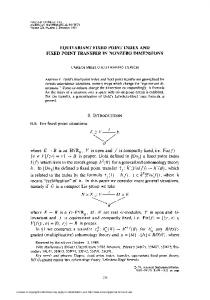
method, we consider also presenting the basins of attraction of the roots. The drawing process for the basins of attraction follows Varona [14]. Typically for the upcoming figures, in squares [2.5, 2.5]2 , we assign a color to each attraction basin of each root. That is, we color a point depending on whether within a fixed number of iteration (here 25) we lie with a certain precision (here 10−3 ) of a given root. If after 25 iterations we do not lie within 10−3 of any given root we assign to the point a very dark shade of purple. The more there are dark shades of purple, the more the points have failed to achieve the required precision within the predetermined number of iteration. 5.1. Examples for Theorem 3. We start with iterative methods of order 2. From Theorem 3, we first want 𝑐0 (𝛼) = 𝛼. We observe that the simplest such function is 𝑐0 (𝑧) = 𝑧. Such a choice has the advantage that derivative of higher order than 2 of this function 𝑐0 (𝑧) will be 0, thus simplifying further computation. This is in fact the choice of function 𝑐0 (𝑧) which leads to Newton’s method and Chebyshev family of iterative methods. We observe however that it is generally possible to consider different choices of functions, although most might be numerically convenient as we will illustrate here. We need 𝑐0 (𝛼) = 𝛼, in such we can also look at 𝑐0 (𝑧) = 𝑧𝑎(𝑧) where 𝑎(𝛼) = 1. In the examples that follow we will look at such functions 𝑎(𝑧). In Table 1, we have considered 3 functions of this kind. We have developed explicit expressions for 𝑓(𝑧) = 𝑧3 −1. Figure 1 presents different graphs for the basins of attraction for these methods. We observe that some of them have a lot of purple points. Now let us consider method of order 3 with 𝑐0 (𝑧) = 𝑧3𝑚+1 with (𝑚 ∈ Z). In this case we obtain Φ3 (𝑧) =

𝑧3𝑚−2 [(3𝑚 − 2) (3𝑚 − 5) 𝑧3 18

(48) −3

− 2 (3𝑚 + 1) (3𝑚 − 5) + (3𝑚 + 1) (3𝑚 − 2) 𝑧 ] ,

𝑓 (𝑧) = 0,

(46)

𝑓 (𝑧) = 𝑧3 − 1.

(47)

and its asymptotic constant is

for

As examples of the preceding results, we present methods of orders 2 and 3 obtained from Theorems 3, 5, and 7. For each

𝐾3 (𝛼; Φ3 ) =

(3𝑚 + 1) (3𝑚 − 2) (3𝑚 − 5) 𝛼. 6

(49)

Examples of basins of attraction are given in Figure 2 for 𝑚 = 0, 1, 2. The smallest asymptotic constant is for 𝑚 = 1.

6

Journal of Complex Analysis

2

2

1

1

0

0

−1

−1

−2

−2 −2

−1

0

1

2

−2

(a) For 𝑚 = 0, 𝑐0 (𝑧) = 𝑧 and its asymptotic constant is 𝛼2

2

2

1

1

0

0

−1

−1

−2

−2 −2

−1 3

(c) For 𝑐0 (𝑧) = 𝑧(𝑒(𝑧

0

−1)

1

−2

2

), the asymptotic constant is −(13/2)𝛼2

−1

0

1

2

(b) For 𝑚 = 1, 𝑐0 (𝑧) = 𝑧4 and its asymptotic constant is −2𝛼2

−1

0

1

2

(d) For 𝑐0 (𝑧) = 𝑧 cos(𝑧3 − 1), the asymptotic constant is (11/2)𝛼2

Figure 1: Basins of attraction for methods of order 2 of Table 1.

5.2. Examples for Theorem 5. Gerlach’s process described in Theorems 5 and 6 leads to Newton’s method for 𝑝 = 2 and Halley’s method for 𝑝 = 3. For our problem we have 𝑁𝐹2 (𝑧) = 𝑧 − 𝑁𝐹3 (𝑧) = 𝑧 −

(𝑧3 − 1) 3𝑧2

, (𝑧3 − 1) /3𝑧2 (1)

1 − (1/2) [1 − ((𝑧3 − 1) /3𝑧2 ) ]

(50)

𝑧3 + 2 . 2𝑧3 + 1 These methods are well known standard methods. For comparison, their basins of attraction are given in Figure 3. =𝑧

5.3. Examples for Theorem 7. To illustrate Theorem 7, we set 𝑑0 (𝑧) = 0 and 𝑑1 (𝑧) = 𝑧𝑘 for 𝑘 ∈ Z, and let us consider methods of orders 2 and 3 to solve 𝑧3 − 1 = 0. Table 2 presents the quantities Ψ𝑝 (𝑧), 𝑁Ψ𝑝 (𝑧), 𝑑𝑝 (𝑧), and 𝐾𝑝 (𝛼; Ψ𝑝 ) for 𝑝 = 2, 3 for this example. We observe that the asymptotic constant of the method of order 2 for 𝑘 = −1 is zero; it means that this method is of an order of convergence higher than 2, and in fact it corresponds to Halley’s method which is of order 3. We observe that methods of order 3 for the values of 𝑘 = −1 and 𝑘 = 2 both correspond to Halley’s method for our specific problem. Examples of basins of attraction are given in Figure 4 for methods of order 2 and in Figure 5 for methods of order 3 using values of 𝑘 = −2, −1, 0, 1, 2, 3.

Journal of Complex Analysis

7

2

1

0

−1

−2 −2

−1

0

1

2

(a) 𝑚 = 0 and its asymptotic constant is (5/3)𝛼 (Chebyshev’s method)

2

1

0

−1

−2 −2

−1

0

1

2

(b) 𝑚 = 1 and its asymptotic constant is −(4/3)𝛼

2

1

0

−1

−2 −2

−1

0

1

2

(c) 𝑚 = 2 and its asymptotic constant is (14/3)𝛼

Figure 2: Methods of order 3 for computing the cubic root with 𝑐0 (𝑧) = 𝑧3𝑚+1 for 𝑀 = 0, 1, 2.

8

Journal of Complex Analysis

2

1

0

−1

−2 −2

−1

0

1

2

(a) 𝑁𝐹2 (𝑧) is Newton’s method

2

1

0

−1

−2 −2

−1

0

1

2

(b) 𝑁𝐹3 (𝑧) is Halley’s method

Figure 3: First two methods for computing the third root with Theorem 5.

Table 2: Method of orders 2 and 3 based on Theorem 3. 𝑁Ψ𝑝 (𝑧) (𝑘 + 2) 𝑧3 − (𝑘 − 1) 𝑧 2 𝑧 (𝑧 − 1) (𝑘 + 3) 𝑧3 − 𝑘 3 𝑘 [(𝑘 + 2) − 𝑘) 𝑧 + − 1) (2𝑘 − 1) − (𝑘 − 4) (𝑘 + 1) 𝑧−3 ] (2 (𝑘 𝑧 3 [(2 − 𝑘) 𝑧3 + (2𝑘 − 1) − (𝑘 + 1) 𝑧−3 ] 𝑧 [(𝑘 + 3) (2 − 𝑘) 𝑧3 + 𝑘 (2𝑘 − 1) − (𝑘 − 3) (𝑘 + 1) 𝑧−3 ] 3 Ψ𝑝 (𝑧)

𝑝

𝑘

3

6. Concluding Remarks In this paper we have presented fixed point and Newton’s methods to compute a simple root of a nonlinear analytic function in the complex plane. We have pointed out that the

𝑑𝑝 (𝑧) 𝐾𝑝 (𝛼; Ψ𝑝 ) 𝑘 + 1 𝑘−3 − 𝑧 (𝑘 + 1) 𝛼2 3 3𝑘2 − 3𝑘 − 8 𝑘−4 3𝑘2 − 3𝑘 − 8 𝑧 𝛼 − 2 54𝑧 3

usual sufficient conditions for convergence are also necessary. Based on these conditions for high-order convergence, we have revisited and extended both Schr¨oder’s methods of the first and second kind. Numerical examples are given to illustrate the basins of attraction when we compute the third

Journal of Complex Analysis

9

2

2

1

1

0

0

−1

−1

−2

−2 −2

−1

0

1

−2

2

(a) 𝑘 = −2 and 𝑑1 (𝑧) = 𝑧−2

2

2

1

1

0

0

−1

−1

−2

−2 −2

−1

0

1

−2

2

(c) 𝑘 = 0 and 𝑑1 (𝑧) = 1

2

1

1

0

0

−1

−1

−2

−2 −1

0

1 2

(e) 𝑘 = 2 and 𝑑1 (𝑧) = 𝑧

0

1

2

−1

0

1

2

(d) 𝑘 = 1 and 𝑑1 (𝑧) = 𝑧

2

−2

−1

(b) 𝑘 = −1 and 𝑑1 (𝑧) = 𝑧−1

2

−2

−1

0

1 3

(f) 𝑘 = 3 and 𝑑1 (𝑧) = 𝑧

Figure 4: Methods of order 2 to illustrate Theorem 7.

2

10

Journal of Complex Analysis

2

2

1

1

0

0

−1

−1

−2

−2 −2

−1

0

1

−2

2

−2

2

1

1

0

0

−1

−1

−2

−2 0

1

−2

2

(c) 𝑘 = 0 and 𝑑1 (𝑧) = 1

2

1

1

0

0

−1

−1

−2

−2 −1

0

1 2

(e) 𝑘 = 2 and 𝑑1 (𝑧) = 𝑧

2

−1

0

1

2

(d) 𝑘 = 1 and 𝑑1 (𝑧) = 𝑧

2

−2

1

(b) 𝑘 = −1 and 𝑑1 (𝑧) = 𝑧

2

−1

0

−1

(a) 𝑘 = −2 and 𝑑1 (𝑧) = 𝑧

−2

−1

2

−2

−1

0

1 3

(f) 𝑘 = 3 and 𝑑1 (𝑧) = 𝑧

Figure 5: Methods of order 3 to illustrate Theorem 7.

2

Journal of Complex Analysis roots of unity. It might be interesting to study the relationship, if there is any between the asymptotic constant and the basin of attraction for such methods.

Conflicts of Interest The authors declare that they have no conflicts of interest.

Acknowledgments This work has been financially supported by an individual discovery grant from NSERC (Natural Sciences and Engineering Research Council of Canada) and a grant from ISM (Institut des Sciences Math´ematiques).

References [1] F. Dubeau and C. Gnang, “Fixed point and Newton’s methods for solving a nonlinear equation: from linear to high-order convergence,” SIAM Review, vol. 56, no. 4, pp. 691–708, 2014. [2] F. Dubeau, “Polynomial and rational approximations and the link between Schr¨oder’s processes of the first and second kind,” Abstract and Applied Analysis, vol. 2014, Article ID 719846, 5 pages, 2014. [3] F. Dubeau, “On comparisons of chebyshev-halley iteration functions based on their asymptotic constants,” International Journal of Pure and Applied Mathematics, vol. 85, no. 5, pp. 965– 981, 2013. [4] E. Schr¨oder, “Ueber unendlich viele algorithmen zur aufl¨osung der gleichungen,” Mathematische Annalen, vol. 2, no. 2, pp. 317– 365, 1870. [5] E. Schr¨oder, “On Infinitely Many Algorithms for Solving Equations,” in Institute for advanced Computer Studies, G. W. Stewart, Ed., pp. 92–121, University of Maryland, 1992. [6] J. F. Traub, Iterative Methods for the Solution of Equations, Prentice-Hall, NJ, USA, Englewood Cliffs, 1964. [7] A. S. Householder, The Numerical Treatment of a Single Nonlinear Equation, McGraw-Hill Book Co., NY, USA, 1970. [8] E. Bodewig, “On types of convergence and on the behavior of approximations in the neighborhood of a multiple root of an equation,” Quarterly of Applied Mathematics, vol. 7, pp. 325–333, 1949. [9] M. Shub and S. Smale, “Computational complexity. On the geometry of polynomials and a theory of cost,” Annales Scien´ tifiques de l’Ecole Normale Sup´erieure. Quatri`eme S´erie, vol. 18, no. 1, pp. 107–142, 1985. [10] M. Petkovi´c and D. Herceg, “On rediscovered iteration methods for solving equations,” Journal of Computational and Applied Mathematics, vol. 107, no. 2, pp. 275–284, 1999. [11] J. Gerlach, “Accelerated convergence in Newton’s method,” SIAM Review, vol. 36, no. 2, pp. 272–276, 1994. [12] W. F. Ford and J. A. Pennline, “Accelerated convergence in Newton’s method,” SIAM Review, vol. 38, no. 4, pp. 658-659, 1996. [13] F. Dubeau, “On the modified Newton’s method for multiple root,” Journal of Mathematical Analysis, vol. 4, no. 2, pp. 9–15, 2013. [14] J. L. Varona, “Graphic and numerical comparison between iterative methods,” The Mathematical Intelligencer, vol. 24, no. 1, pp. 37–46, 2002.

11

Advances in

Operations Research Hindawi Publishing Corporation http://www.hindawi.com

Volume 2014

Advances in

Decision Sciences Hindawi Publishing Corporation http://www.hindawi.com

Volume 2014

Journal of

Applied Mathematics

Algebra

Hindawi Publishing Corporation http://www.hindawi.com

Hindawi Publishing Corporation http://www.hindawi.com

Volume 2014

Journal of

Probability and Statistics Volume 2014

The Scientific World Journal Hindawi Publishing Corporation http://www.hindawi.com

Hindawi Publishing Corporation http://www.hindawi.com

Volume 2014

International Journal of

Differential Equations Hindawi Publishing Corporation http://www.hindawi.com

Volume 2014

Volume 2014

Submit your manuscripts at https://www.hindawi.com International Journal of

Advances in

Combinatorics Hindawi Publishing Corporation http://www.hindawi.com

Mathematical Physics Hindawi Publishing Corporation http://www.hindawi.com

Volume 2014

Journal of

Complex Analysis Hindawi Publishing Corporation http://www.hindawi.com

Volume 2014

International Journal of Mathematics and Mathematical Sciences

Mathematical Problems in Engineering

Journal of

Mathematics Hindawi Publishing Corporation http://www.hindawi.com

Volume 2014

Hindawi Publishing Corporation http://www.hindawi.com

Volume 2014

Volume 2014

Hindawi Publishing Corporation http://www.hindawi.com

Volume 2014

#HRBQDSDĮ,@SGDL@SHBR

Journal of

Volume 201

Hindawi Publishing Corporation http://www.hindawi.com

Discrete Dynamics in Nature and Society

Journal of

Function Spaces Hindawi Publishing Corporation http://www.hindawi.com

Abstract and Applied Analysis

Volume 2014

Hindawi Publishing Corporation http://www.hindawi.com

Volume 2014

Hindawi Publishing Corporation http://www.hindawi.com

Volume 2014

International Journal of

Journal of

Stochastic Analysis

Optimization

Hindawi Publishing Corporation http://www.hindawi.com

Hindawi Publishing Corporation http://www.hindawi.com

Volume 2014

Volume 2014