Fixed-Precision Approximate Continuous Aggregate Queries in Peer-to-Peer Databases Farnoush Banaei-Kashani
Cyrus Shahabi
Computer Science Department University of Southern California Los Angeles, CA 90089 Email:
[email protected]
Computer Science Department University of Southern California Los Angeles, CA 90089 Email:
[email protected]
Abstract—In this paper, we propose an efficient sample-based approach to answer fixed-precision approximate continuous aggregate queries in peer-to-peer databases. First, we define practical semantics to formulate fixed-precision approximate continuous aggregate queries. Second, we propose “Digest”, a two-tier system for correct and efficient query answering by sampling. At the top tier, we develop a query evaluation engine that uses the samples collected from the peer-to-peer database to continually estimate the running result of the approximate continuous aggregate query with guaranteed precision. For efficient query evaluation, we propose an extrapolation algorithm that predicts the evolution of the running result and adapts the frequency of the continual sampling occasions accordingly to avoid redundant samples. We also introduce a repeated sampling algorithm that draws on the correlation between the samples at successive sampling occasions and exploits linear regression to minimize the number of the samples derived at each occasion. At the bottom tier, we introduce a distributed sampling algorithm for random sampling (uniform and nonuniform) from peerto-peer databases with arbitrary network topology and tuple distribution. Our sampling algorithm is based on the Metropolis Markov Chain Monte Carlo method that guarantees randomness of the sample with arbitrary small variation difference with the desired distribution, while it is comparable to optimal sampling in sampling cost/time. We evaluate the efficiency of Digest via simulation using real data.
I. I NTRODUCTION A peer-to-peer database is a fragmented database which is distributed among the nodes of a peer-to-peer network, with both the data and the network dynamically changing. In this paper, we focus on answering continuous aggregate queries in peer-to-peer databases, where the underlying peerto-peer network of the database is inherently unstructured (as opposed to DHT-based structured peer-to-peer networks). Continuous queries [20] allow users to obtain new results from the database without having to issue the same query repeatedly. Continuous queries are especially useful with peerto-peer databases which inherently comprise of large amounts of frequently changing data. For example, in a weather forecast system with thousands of interconnected stations the system administrator can issue a continuous aggregate query of the form: “Over next 24 hours, notify me whenever the average temperature of the area changes more than 2 o F.”
Or in a peer-to-peer computing system with distributed resources, users can issue the following query to determine when there is enough memory space available to schedule their tasks: “Notify me whenever the total amount of available memory is more than 4GB.” However, considering the large size and the high rate of change in peer-to-peer databases, exact continuous aggregate queries are inevitably inefficient, if not infeasible. Exact answers are rarely necessary, and even if needed, a consistent approximation can converge to the exact result with arbitrary precision. Therefore, in this paper we consider approximate continuous aggregate queries. Previous approaches for approximate query answering are not applicable to peer-to-peer databases. The model based approaches [6] are parameterized, where with peer-to-peer databases parameters are unknown and variable. The histogram based [11] and the precomputed-sample based [13] data reduction approaches are not appropriate either. Although dynamically updated, with the high rate of change in peer-to-peer databases maintaining histograms and precomputed samples is intolerably costly. The large set of techniques proposed for approximate continuous aggregate query over data streams [2] naturally assume the data are collected centrally and are being received in sequence, where none of these assumptions hold for the data in peer-to-peer databases. Finally, the current onthe-fly sampling approaches, mostly developed for query size estimation [14], are limited to snapshot (or one-time) aggregate queries. In this paper, we propose an approach for answering fixedprecision approximate continuous aggregate queries by on-thefly sampling from peer-to-peer databases. Our query answering system, called Digest, evaluates approximate continuous aggregate queries by continual execution of the approximate snapshot aggregate queries, where each snapshot query is evaluated by sampling the database. The snapshot queries probe the database and accordingly the running result of the continuous query is updated. As we elaborate below, with continuous queries the main issue transcends how to execute each snapshot query, but how to execute snapshot queries continually such that while the fixed precision requirements of the continuous query are guaranteed, the query is answered efficiently by deriving minimum number of samples.
With fixed-precision approximate continuous aggregate queries, the required (or fixed) precision of the approximate result is defined by the user in terms of 1) the resolution of the result in capturing the changes of the actual running aggregate value (e.g., the result reflects the changes of the average temperature iff a change is more than 2 o F), and 2) the confidence (or accuracy) of the result at each time as compared to the exact aggregate value at that time. Using continual snapshot queries to answer such queries, the resolution of the result is determined by the frequency of the snapshots, and the confidence of the result depends on the number of the samples derived to approximate the result of each snapshot query. Therefore, for efficient evaluation of the continuous queries while guaranteeing the fixed precision, both the frequency of the snapshot queries and the number of the samples derived at each snapshot query must be minimized while the resolution requirement and the confidence requirement of the query are still satisfied, respectively. Digest provides solutions for both of these optimization problems. Digest is implemented as a two-tier system, with a sampling operator at the bottom tier and a query evaluation engine at the top tier. The sampling operator implements a distributed sampling algorithm to derive arbitrary random samples from the peer-to-peer databases (with arbitrary topology and tuple distribution). The query engine uses the samples collected from the database to evaluate the snapshot queries. To minimize the frequency (or equivalently, the number) of the snapshot queries, the query engine exploits an extrapolation algorithm that predicts the evolution of the running aggregate value based on its previous behavior and adapts the frequency of the continual snapshot queries accordingly. With this approach, the more varying the aggregate value, the more becomes the frequency of the snapshot queries in order to maintain the resolution of the result, and when the aggregate value is steady the frequency of the snapshot queries decreases accordingly to avoid redundant sampling. On the other hand, to minimize the number of the samples derived at each snapshot query, the query engine employs a repeated sampling algorithm. Repeat sampling draws on the observation that across successive snapshot queries the values of the database tuples are expected to be autocorrelated and, therefore, exploiting the regression of the value of a sampled tuple at the current query on that of the previous query can improve the accuracy of the current estimate. Repeated sampling uses regression estimation to achieve the required confidence using fewer samples as compared with the straightforward independent sampling which ignores the correlation between the snapshots. We study both the extrapolation algorithm and the repeated sampling algorithm analytically. Besides, we demonstrate their effectiveness via simulation using real data. We show that the combined effect of our extrapolation and repeated sampling algorithms can improve the efficiency of the query evaluation up to 320% as compared with the straightforward continual query execution with fixed frequency and independent sampling.
The remainder of this paper is organized as follows. In Section II, we define the semantics of the fixed-precision approximate continuous aggregate queries. Section III presents an overview of the Digest architecture. In Section IV, we describe the query evaluation component of Digest, and follow by explaining the distributed sampling component in Section V. Section VI presents the results of our empirical study on Digest. In Section VII, we briefly discuss the remaining related work. Finally, Section VIII concludes the paper and discusses the future directions of this research. II. A PPROXIMATE C ONTINUOUS Q UERY We model an unstructured peer-to-peer network as an undirected graph G(V, E) with arbitrary topology. The set of vertices V = {v1 , v2 , . . . , vr } represent the set of the network nodes, and the set of edges E = {e1 , e2 , . . . , eq } represent the set of the network links, where ei = (vj , vk ) is a link between vj and vk . As nodes autonomously join and leave the network, the member-set of V , and accordingly, that of E vary in time. Consequently, the set sizes r and q are also variable and unknown a priori. We assume the rate of the changes in G is relatively low as compared to the sampling time (i.e., the time required to draw a sample from the peer-topeer database), such that the network can be assumed almost static during each sampling occasion (although it may change significantly between successive sampling occasions). For a peer-to-peer database stored in such an unstructured peer-to-peer network, without loss of generality we assume a relational model. Suppose the database consists of a single relation R = {u1 , u2 , . . . , uN }. R (a multiset) is horizontally partitioned and each disjoint subset of its tuples is stored at a separate node. The number of tuples stored at the node vi is denoted by mvi . The member-set of R also varies in time; the changes are either due to the changes of V , as nodes with new content join the network (as if inserting tuples) and existing nodes leave and remove their content (as if deleting tuples), or as the existing nodes autonomously modify their local content by insertion, update, and deletion. With such a model for peer-to-peer databases, we define our basic query model for the continuous aggregate queries as follows. Consider the queries of the form: SELECT op(expression) FROM R where op is one of the aggregate operations AVG, COUNT, or SUM, and expression is an arithmetic expression involving the attributes of R. Suppose Q is an instance of such queries. Assuming a discrete-time model (i.e., the time is modelled as a discrete quantity with some fixed unit), the snapshot aggregate query Qt is the query Q evaluated at time t. Correspondingly, the continuous aggregate query Qc is the query Q evaluated continuously (i.e., repeated successively without intermission) for all t ≥ t0 , where t0 is the arrival time of Qc . The result of Qc is X[t], a discrete-time function where for all t ≥ t0 , X[t] is the aggregate-value result of the snapshot query Qt . For instance, in a peer-to-peer computing system each node (a node consists of one or more computing units) keeps
tu
tu
0
tu2
1
tu
3
tu tu 4
tu
5
6
tu tu 7
8
tu
9
tu
10
tu
11
tu
12
Aggregate Value
ε
∆X2
Exact Result X[t] δ
∆X1
t0 =
0
1
2
3
^
Approximate Result X[t]
4
5
6
7
8
9
10
11
12
13
14
15
16
17
18
19
20
Time
Fig. 1.
Fixed-Precision Approximate Continuous Aggregate Query
a current record of its available resources by maintaining tuples of the form ui = hcpu, memory, storage, bandwidthi, one tuple for each local computing unit. Considering R(cpu, memory, storage, bandwidth) as a single-relation peer-to-peer database representing the resources available in such a peer-to-peer computing system, the following continuous query returns X, the total amount of the space currently available throughout the system, as a function of time: SELECT SUM(memory + storage) FROM R With a fixed-precision approximate version of the exact continuous query Qc defined above, the exact result X[t] is b with guaranteed precision approximated by an estimate X[t] (see Figure 1). Our model for approximate queries includes three extra user-defined parameters, δ, ², and p, to specify the desired precision of the estimation. With δ, user specifies b in capturing the incremental changes in the resolution of X[t] X[t] as it evolves in time. To answer an exact query, X[t] is updated (i.e., re-evaluated by snapshot query) at every time instant t, regardless of the amount of change in X since the last update at t−1. However, with approximate queries smaller changes below some threshold may be insignificant to the user/application and, therefore, not required to be reflected b in the estimated result X[t]. The parameter δ defines this application-specific threshold. Suppose tui is the most recent b is updated (initially, tu = t0 ). time at which the result X[t] 0 For t > tui , the approximate query is not required to re-update the result until t = tui+1 , where tui+1 is the earliest time at which ∆X ≥ δ (by definition ∆X = |X[tui+1 ]−X[tui ]|). For b can be estimated all times t in the interval (tui , tui+1 ), X[t] b = without update/re-evaluation, e.g., by “holding” (i.e., X[t] b u ]) or interpolation. With this semantic for approximation, X[t i the smaller changes of X during the intervals (tui , tui+1 ) for i = 0, 1, 2, 3, . . . are filtered out of the estimated result. Back to our running example mentioned above, changes on the order of several megabytes in the total space may not be noteworthy for a distributed task scheduling application and/or may be too costly to monitor. In such a case, e.g., δ = 1GB might be an effective choice to formulate an approximate query that is both useful and practical. It is important to note that in addition to allowing for optimization of the query efficiency, δ
provides useful functionality to the user. Consider each update of the running query result raises an alarm for the user. With δ, user can avoid false alarms. For example, consider a scenario where a weather reporter does not want to report the average temperature unless the change in the average is more than δ = 5o F . Next, the parameter ² indicates the maximum tolerable b absolute error in the estimate X[t] at each time tui . The b u ] − X[tu ]| ≤ ² approximate query should guarantee |X[t i i for all i. The interval [X[tui ] − ², X[tui ] + ²] is termed the confidence interval of the estimation at time tui , with X[tui ] − ² and X[tui ] + ² as the lower and upper confidence limits, respectively. The provided guarantee is probabilistic and with the parameter p user specifies the desired confidence level b u] of the guarantee, i.e., the probability that the estimation X[t i is actually confined within the confidence interval. The userdefined parameters ² and p together determine the required b u ]. Note that, approximate confidence of the estimate X[t i query generalizes exact query; an exact query is an approximate query with δ = 0, ² = 0, and p = 1. To answer an exact continuous aggregate query, snapshot queries must be executed continuously, each evaluated for an exact result; hence, termed continuous-exact snapshot queries. Alternatively, an approximate continuous aggregate query can be answered by executing the more flexible and general continual-approximate snapshot queries. With continual-approximate queries, the less frequent the snapshot queries and the less accurate the approximation by each snapshot query, the less the cost of evaluating the continuous aggregate query, but also the less the precision (i.e., the resolution and the confidence, respectively) of the result. That allows a trade-off between the precision and the cost of obtaining the result, such that while the fixed-precision approximate query is correctly satisfied, the cost of evaluating the query can be optimized for efficiency. An extreme case of the trade-off is with continuous-exact snapshot queries to answer exact continuous aggregate queries. With continuous-exact snapshot queries, both the frequency of the snapshot queries and the accuracy of the approximation by each snapshot query are maximal, such that the estimated b result of the continuous query is exact (i.e., X[t] = X[t]) while it costs the most to evaluate. Next, we present Digest, a query answering system that executes continual-approximate snapshot queries by sampling the database, and optimizes the frequency and accuracy of the snapshot queries to answer approximate continuous aggregate queries both correctly (with guaranteed precision) and efficiently. III. D IGEST: OVERVIEW Figure 2 depicts the two-tier architecture of Digest. Each node of the peer-to-peer database operates its own individual instance of Digest to answer the continuous queries received from the local user. As discussed in Section I, the query evaluation engine at the top tier exploits an extrapolation algorithm (see Section IV-A on continual querying) and a repeated sampling algorithm (see Section IV-B on approximate querying) to optimize the number of the samples derived to
Digest
Query
Sample-based Query Evaluation Engine
Top Tier
Random Sampling Operator
Bottom Tier
Samples Peer-to-Peer Database
Fig. 2.
Two-Tier Architecture of Digest
answer continuous aggregate queries. In addition to the query evaluation engine, Digest benefits from a sampling operator at the bottom tier that (in collaboration with other instances of Digest distributed throughout the peer-to-peer network) efficiently derives random samples from the peer-to-peer database. Here, we describe the interface of the sampling operator; the distributed sampling algorithm developed to implement the sampling operator itself is presented in Section V. The sampling operator of Digest implements a distributed sampling algorithm to draw random samples (sample nodes and correspondingly sample tuples) from the peer-to-peer databases with arbitrary network topology and tuple distribution. The interface of the sampling operator is defined as follows. First, consider a generic weight function w that assigns a weight wv to each node v of the database. For instance, w1 = {∀v ∈ V | wv = 1} is a uniform weight function, and w2 = {∀v ∈ V | wv = mv } is a (possibly) nonuniform weight function with which each node is weighted according to the number of the tuples mv stored at the node. We assume that with w the weight of each node is a function of the local properties of the node (such as the content-size mv of the node, the degree of connectivity of the node, the reputation of the node, the accuracy and relevance of the tuples stored at the node, etc.), and the assigned weight is not necessarily normalized. Given such a weight function w as input, once invoked the sampling operator S randomly P derives a sample node v from V such that pv = wv / u∈V wu , where pv is the probability of sampling the node v. In other words, the distribution of the sampling probability among the nodes is proportional to the distribution of the weight according to the desired (uniform or nonuniform) weight function w. As we show in Section V, with our distributed sampling algorithm each node only needs to know the weights of its local neighbors; hence, no need to acquire global information. While the sampling operator S proposed in this paper can be used to draw sample nodes based on any generic weight function, as we discuss in Section IV-B1 with Digest we employ S to draw uniformly random sample tuples from R using the weight function w= {∀v ∈ V | wv = mv }, where mv is the number of tuples stored at each node. For this purpose, first S is invoked with the weight function w to derive a sample node with a sampling probability proportional to its contentsize. Thereafter, the content of the sampled node is uniformly sampled to derive a sample tuple. The combination of the two
samplings, i.e., the distributed node sampling via S and the local tuple sampling from the sampled node, uniquely specifies the random distribution of the sampled tuple in the entire R, which in this case is uniform as desired. This sampling scheme is termed two-stage sampling [7]. Instead, one can use cluster sampling with which all tuples of the sampled node are drawn as a batch sample. However, since with most P2P applications the contents of a node are highly correlated (high intra-cluster and low inter-cluster correlation), cluster sampling results in imprecise estimations with these applications. Therefore, with Digest we prefer two-stage sampling to cluster sampling. With the above two-stage sampling scheme, sampling the tuples stored at the sampled node is performed locally; hence, it is standard and inexpensive. The sampling operator S, which implements the more complicated and costly distributed node sampling, ensures suboptimal performance (comparable to that of the optimal sampling) in terms of communication cost and sampling time, while guaranteeing randomness of the derived sample node with arbitrary small error (i.e., variation difference) as compared to the desired sampling probability distribution (see Section V for details). IV. S AMPLE - BASED Q UERY E VALUATION As mentioned in Section I, to evaluate an approximate continuous query one needs to provide solution for two subproblems: 1) continual querying, i.e., to determine when to execute the next snapshot query, and 2) approximate querying, i.e., to minimize the number of samples required to answer each snapshot query. An integrated technique that incorporates solutions for the two sub-problems simultaneously is ideal but complicated. With Digest, we address the two sub-problems separately. First, at each occasion Digest uses an extrapolation algorithm to decide when to execute the next snapshot query (Section IV-A). Thereafter, Digest uses a repeated sampling algorithm to evaluate the snapshot query with the minimum number of samples required to satisfy the confidence requirements of the query (Section IV-B). This process is repeated while the continuous query is running. Below, we describe these algorithms. A. Continual Querying Suppose the most recent snapshot query is executed at time tui = k (see Figure 3). For continual querying, we should predict the next update time tui+1 such that |X[tui+1 ]− X[tui ]| ≥ δ. To predict tui+1 , in brief our approach is to fit a curve to the previously observed values of X to predict its values in the near future with guaranteed error bounds. If the ratio of the change/variation of X[t] in time is unbounded, the future values of X are unpredictable and, therefore, inevitably continual querying reduces to continuous querying to ensure the required resolution. However, the aggregate value X[t] is expected to be a smooth function of time with considerable autocorrelation in short time intervals that bounds its variation (e.g., consider the variation of the total amount of the available space in a peer-to-peer computing system). Hereafter, by convention we model such a smooth function X[t] with bounded
tu
tu
i-3
i-2
tu
tu
i-1
tu
i
B. Approximate Querying
i+1
Aggregate Value
X[t] Pn[t]
∆Pn [t]
δ
Rn [t]
1) Independent Sampling: To provide the background for explaining the repeated sampling algorithm, in this section we briefly review the query evaluation process for an approximate AVG query based on the classical independent sampling algorithm. With the independent sampling algorithm, to answer an AVG snapshot query Qt SELECT AVG(expression) FROM R
k-8
k-7
k-6
k-5
k-4
k-3
k-2
k-1
k
k+1
k+2
k+3
k+4
Time k+5
Fig. 3. Computing tui+1 by Polynomial Extrapolation: at t = tui+1 , we have |∆Pn [tui+1 ]| + |Rn [tui+1 ]| > δ
variation as an analytic function of time, i.e., we assume X[t] possesses derivatives of all orders and agrees with its Taylor series in the neighborhood of every point. Assuming that X[t] is an analytic function, our continual querying algorithm predicts the evolution of the analytic function X[t] by polynomial extrapolation using the Taylor series expansion. Based on the Taylor’s theorem, at the neighborhood of tui , X[t] can be approximated by a degree-n Taylor polynomial Pn [t]: (t − tui )2 00 Pn [t] = X[tui ] + (t − tui )X 0 [tui ] + X [tui ] 2! (t − tui )n (n) + ... + X [tui ] (1) n! The upper bound error for this approximation of X[t] with the Taylor polynomial is the Lagrange remainder Rn [t], such that |X[t] − Pn [t]| < |Rn [t]|, where: (t − tui )n+1 (n+1) Rn [t] = X [ct ] (2) (n + 1)! (n+1) with ct ∈ [tui , t] a constant minimizing X [t] in this interval. To find tui+1 , first Pn [t] is computed by fitting a degree-n polynomial to n+1 previous values of X[t] at t = (k−n), t = (k − n + 1), ..., and t = k. We use the well-known LevenbergMarquardt Method (based on non-linear least squares fitting via trust regions) for fitting. This method is known for robust estimation of the Taylor polynomial. Note that the exact values of X[t] are unknown unless the snapshot queries are exact. Instead of the exact values, assuming sufficiently accurate approximate snapshot results, we compute Pn [t] using n + 1 b at t = tu , t = tu previous values of X[t] , ..., and i−n i−n+1 t = tui (n = 3 in Figure 3). Next, having Pn [t] as an approximation with bounded error for X[t], tui+1 is derived by extrapolation as the minimum t satisfying: |Pn [t] − Pn [tui ]| + |Rn [t]| > δ (3) Note that the upper bound error |Rn [t]| of the polynomial approximation is a decreasing function of n. Therefore, the higher the degree of the polynomial approximation, the tighter is the error bound and, thus, the predicted update time tui+1 is less conservative, which makes the continual querying more efficient. Also, while t < tun , a degree-n polynomial approximation is not applicable. During the bootstrapping period, i.e., the interval [tu0 , tun ), our continual querying algorithm implements continuous querying instead of continual querying.
n sample tuples u1 , u2 , ..., un are derived from R, uniformly random and with replacement. The time interval (beginning at t) during which the database is probed to draw samples for evaluating Qt is called the sampling occasion for Qt . During the sampling occasion, each sample is drawn by first calling the sampling operator S with the weight function w = {∀v ∈ V | wv = mv } to derive a sample node with a sampling probability proportional to its content-size. Next, the content of the sampled node is uniformly sampled to derive a sample tuple. Suppose the value of the expression when applied to the sample tuple ui is denoted by yi . Based PN on the derived samples, the result (X =) Y = 1/N i=1 yi of the AVG query is estimated by the unbiased and consistent estimator: n X b Y = 1/n y (4) i
The number of the samplesi=1 n is computed such that with b probability p the estimate Y is within the confidence interval [Y − ², Y + ²]. One can use the standard central limit theorem PN to compute n. Let σ 2 = 1/N i=1 (yi − Y )2 be the true Pn variance of yi in R, and σ b2 = 1/n i=1 (yi − Yb )2 the estimated variance. For sufficiently large n, it follows from the central limit theorem that the random variable Yb has a normal distribution with mean Y and variance σ 2 /n, or equivalently, √ the standardized random variable n(Yb − Y )/σ has a normal distribution with mean 0 and variance 1. Therefore: ¯ (¯ √ ) ¯ n(Yb − Y ) ¯ ²√n ¯ ¯ b Pr{|Y − Y | ≤ ²} = Pr ¯ ¯≤ ¯ ¯ σ σ µ ¶ √ ² n ≈ 2 Φ( ) − 1/2 (5) σ b where Φ is the standard cumulative normal distribution function. Let lp be the (p + 1)/2 quantile of this distribution (i.e., Φ(lp ) = (p + 1)/2). To derive n, we set the rightmost term in Equation 5 equal to p and solve the equation for n: ¶2 µ σ blp (6) n= ² 2) Repeated Sampling: With independent sampling, each snapshot query is answered independently, disregarding the results and the samples derived for the previous queries. However, across successive queries the values of the database tuples are expected to be autocorrelated and, therefore, exploiting the regression of the value of a sampled tuple at the current sampling occasion on that at the previous occasion can improve the accuracy of the current estimate. Alternatively, by regression estimation one can achieve the same accuracy/confidence
using fewer samples at each sampling occasion; hence, more efficient query evaluation. Repeated sampling relies on this observation to improve the efficiency of independent sampling while still satisfying the confidence requirement of the query. Below, we explain the repeated sampling algorithm in details for evaluation of the AVG queries. Other types of aggregate queries are evaluated similarly. We begin with regression estimation for the evaluation of the 2nd snapshot query (i.e., the special bootstrapping snapshot query) of a continuous aggregate query. Later, we extend the analysis for evaluation of the general k th snapshot query. a) Evaluating 2nd Snapshot Query: Suppose the sampleset is of size n in both the first and the second sampling occasions of a continuous AVG query. Let uik denote the state of the sampled tuple ui at occasion k (i.e., the current attribute-values of the tuple ui at occasion k), and let yik denote the corresponding value of uik when evaluated by the expression in the AVG query at occasion k. At the first occasion, there is no prior information to utilize. Therefore, all n samples u1 , u2 , ..., un are new samples derived from the database and the result of the first snapshot query is simply estimated based on the independent sampling algorithm using u11 , u21 , ..., un1 as the samples. At the second occasion, each sampled tuple ui is either replaced by a new sample ui0 from the database (with the current state ui0 2 ), or retained and reevaluated to its current state ui2 . Thus, the sample-set at the second occasion consists of n samples u1 , ..., ug , ug0 , ..., un0 , where g is the number of retained samples. A new sample ui0 must be derived using the sampling operator S and incurs communication overhead to locate, whereas a retained sample ui is already located and is only retrieved to be re-evaluated (to refresh ui1 to ui2 ) after a possible state update in between the two sampling occasions. If a sample tuple is deleted or the node storing the tuple leaves the network, the tuple is always replaced. Repeated sampling uses the current state of the new samples, i.e., ug0 2 , ..., un0 2 , for regular estimation as in the first occasion, while utilizing the current state of the retained samples, i.e., u12 , ..., ug2 , for regression estimation (where yi2 regresses on yi1 as the auxiliary regression variate). The final estimate of the repeated sampling algorithm for the result of the second snapshot query is a combined estimate, a weighted sum of the regular estimate and the regression estimate from the new portion and the retained portion of the sample-set, respectively. With the above estimation scheme, an optimal sample replacement policy is required to determine the proportion of the new and retained portions of the sample-set such that the combined estimate of the result is optimal (i.e., the most accurate estimate with minimum variance). With two extreme cases of the replacement policy, the samples are either all replaced or all retained. As we show below, none of these policies are optimal. With repeated sampling we establish the optimal replacement policy as follows. Suppose among n samples at the k th sampling occasion (here k = 2), g samples are retained from the previous occasion and the rest f samples (‘f ’ for fresh)
Estimator Yb 2f = y 2f Yb 2g = y 2g + b(y 1 − y 1g )
Variance σ b2 f σ b 2 (1−b ρ2 ) g
= +
2 ρb2 σbn
1 W2f
=
1 W2g
TABLE I R EGULAR AND R EGRESSION E STIMATORS AT 2nd O CCASION
are new samples. Let y kf , y kg , and y k denote the average value of the samples in the new portion, the retained portion, and the entire sample-set (both portions together) at the k th sampling occasion, respectively. Correspondingly, the values of the regular estimate, regression estimate, and the combined estimate for the result Y k of the k th snapshot query are denoted by Yb kf , Yb kg , and Yb k , respectively. The estimators Yb 2f and Yb 2g and their Pncorresponding variances are defined in Table I. σ b22 = 1/n i=1 (yi2 − y 2 )2 is an PN estimate of the true variance σ22 = 1/N i=1 (yi2 − Y 2 )2 of yi in R at the second occasion, and we have σ b2 ≈ σ b b (= σ b1 ). The estimator Y 2f is simply the average value of the samples y 2f in the new portion of the sample-set. For the regression estimate Yb , we consider a linear regression 2g
σ b
with the regression coefficient b = σb1,2 2 . The parameter b is 1 σ an estimate of the true regression coefficient B = σ1,2 2 , where 1 σ1,2 is the covariance of yi1 and yi2 in the entire R, and σ b1,2 σ b is an is its estimate in the sample-set. Similarly, ρb = σb11,2 σ b2 σ estimate of the true correlation coefficient ρ = σ11,2 . σ2 The combined estimate Yb 2 is derived as the sum of the two independent estimates Yb and Yb weighted inversely 2f
2g
by their variance: Yb 2 = αYb 2f + (1 − α)Yb 2g where α = of Yb is:
W2f W2f +W2g .
(7)
By the least squares theory the variance
2
1 W2f + W2g which from Table I works out as: σ b2 (n − g ρb2 ) var(Yb 2 ) = 2 (8) n − g 2 ρb2 The minimum variance varmin (Yb 2 ) is calculated from Equation 8 by derivation with respect to g. This gives the optimal partitioning of the sample-set as: p n 1 − ρb2 n p p fopt = (9) gopt = 1 + 1 − ρb2 1 + 1 − ρb2 and with optimal partitioning, the minimum variance is derived as: p σ b2 varmin (Yb 2 ) = (1 + 1 − ρb2 ) (10) 2n Note that if g = 0 (all samples replaced, like independent sampling) or f = 0 (all samples retained), the estimate variance (see Equation 8) is equal to that of the independent sampling, i.e., σ b2 /n (≈ σ 2 /n). However, with optimal partitioning (g = gopt ) repeated sampling improves the variance with the ratio: var(Yb 2 ) =
p
(b σ 2 /n) − varmin (Yb 2 ) 1 − 1 − ρb2 p = (11) 1 + 1 − ρb2 varmin (Yb 2 ) Based on Equation 11, depending on the correlation |b ρ| (≤ 1) between values of the tuples at successive occasions, repeated sampling can improve the accuracy of the estimation over that of the independent sampling by up to 100% (with maximum correlation |b ρ| = 1). Also, as the correlation |b ρ| increases, with optimal partitioning a larger portion of the samples are retained because regression estimation is more effective. However, unless the correlation is maximum, repeated sampling replaces a considerable portion of the samples to account for the tuple insertions, deletions, and pathological updates. b) Evaluating k th Snapshot Query: Query evaluation at the k th occasion is a generalization of that of the second occasion. Details are included in the extended version of this paper. β=
V. R ANDOM S AMPLING O PERATOR Given a weight function w = {∀v ∈ V | wv } as input, the sampling operator S should randomly derive a sample node v from P V with the sampling probability distribution pv = wv / u∈V wu . We implement our sampling operator based on a distributed sampling algorithm inspired by the Markov Chain Monte Carlo (MCMC) methods for sampling from a desired probability distribution. To sample from a distribution, first an MCMC method constructs a Markov chain that has the desired distribution as its stationary distribution. With such a Markov chain, starting a traversal of the chain from any initial state, under certain conditions the distribution of the covered states of the chain converges to the stationary distribution of the chain after a sufficiently large number of steps. Once converged, the current state is returned as a sample from the desired distribution. With our distributed sampling algorithm, we consider a peer-to-peer network as a Markov chain, with nodes as the states of the chain, and links as the transitions between the states. Also, our algorithm uses random-walking sampling agents that are forwarded from node to node to emulate the state transition process. To sample the peer-to-peer database, the sampling operator at a node initiates a random walk (a sampling agent). If the forwarding probabilities of the random walk (corresponding to the transition probabilities of the constructed Markov chain) are properly assigned such that the stationary distribution of the walk is equivalent to the desired sampling distribution pv , after a sufficiently large number of steps the distribution of the nodes covered by the random walk converges to pv and the current node is returned to the originating node as the sampled node. In the rest of this section, first we describe how our distributed sampling algorithm employs the Metropolis Markov Chain construction algorithm to assign the forwarding probabilities of the random walk for the desired stationary distribution pv . Second, we present our result that determines the number of steps required to converge to the desired distribution with arbitrary difference.
A. Forwarding Probabilities Let the undirected connected graph G(V, E) model a peerto-peer network with arbitrary topology. A random walk that starts at a node v0 (the originating node), arrives at a node vt at time t and with certain forwarding probability moves to a neighbor node vt+1 at time t + 1. Suppose πt denotes the distribution of the node vt such that πt (i) = Pr(vt = i), for all i ∈ V . Let P = (Pij ), i, j ∈ V , denote the forwarding matrix of the random walk, where Pij is the probability that the random walk moves from node i to node j. Pij = 0 if i and j are not adjacent. By definition, we have πt+1 = πt P = π0 P t+1 , where π0 is the distribution of the originating node v0 . The following existence result is classic [17]: Theorem 1: If P is irreducible (i.e., any two nodes are mutually reachable by random walk) and P is aperiodic (which will be if G is non-bipartite), then πt converges to the unique stationary distribution π such that πP = π independent of the initial distribution π0 . The Metropolis algorithm [16] is designed to assign the forwarding probabilities Pij such that the stationary distribution π corresponds to a desired distribution (uniform or nonuniform) such as pv : Theorem 2: Consider the graph G(V, E) and let di denote the degree of the node i in G. For each neighbor j of i, the forwarding probability Pij , i 6= j, is defined as follows: ( p 1 1 if dpii ≤ djj 2 ( di ) Pij = (12) p p p j 1 1 if dii > djj 2 ( dj )( pi ) P and Pii = 1 − j∈neighbors(i) Pij . Then, with the forwarding matrix P , pv is the unique stationary distribution of the random walk on G. The proof for Theorem 2 is complicated [16]. Intuitively, the Metropolis algorithm modifies a regular random walk with uniform forwarding probability to a biased random walk with forwarding probabilities that depend on the desired sampling probability of the neighbor nodes. The Metropolis forwarding matrix P is irreducible [9]. Also, the laziness factor 1/2 adds a virtual self-loop to each node of the G, which makes G nonbipartite and P aperiodic. Thus, convergence of the Metropolis follows from Theorem 1. Note that using the Metropolis algorithm, S implements a fully distributed sampling process with which it does not P require to know/compute the global P normalization factor w (to calculate p = w / u v v u∈V u∈V wu ) in order to assign the forwarding probabilities Pij . Each node i determines its local forwarding probabilities Pij (j is a neighbor of i) individually and only based on the local information. According to Equation 12, to determine Pij , i only needs to know the ratio wj /wi (= pj /pi ), which it computes by obtaining the weight wj from its neighbor j. B. Convergence Time To determine how rapidly πt converges to pv , first consider the following definitions and the subsequent classic result (Theorem 3):
Definition 1: The total-variance difference (or simply variance difference) betweenPtwo distributions πt and pv is defined as kπt , pv k = 12 maxv0 i |πt (i) − pi |. The variance difference is a measure to quantify the total difference between two probability distributions, and we have 0 ≤ kπt , pv k ≤ 1. Definition 2: For γ > 0, the mixing time is defined as τ (γ) = min{t|∀t0 ≥ t, kπt0 , pv k ≤ γ}. The mixing time τ (γ) is the time (i.e., number of time steps) it takes for πt to converge to pv to within the difference γ, such that kπt , pv k ≤ γ. The following theorem bounds the mixing time when the random walk is on a graph G with arbitrary topology [10]: Theorem 3: Let pvmin = mini pi , then τ (γ) ≤ θP−1 log((pvmin γ)−1 ), where θP is the eigengap of the forwarding matrix P . The eigengap of P is defined as θP = 1 − |λ2 |, where λ2 is the second eigenvalue of the matrix. Thus, the larger the eigengap, the more rapidly the random walk converges to the desired distribution. However, computing the exact eigengap of P for peerto-peer networks with large size and dynamic topology is difficult, if not infeasible. Instead, one can utilize the geometric bounding approach [10] to derive a bound for the eigengap. Considering power-law graph as a generic and realistic model for the topology of the peer-to-peer networks [19], we use the geometric bounding approach to derive the mixing time (or convergence time) of the random walk on a graph G with power-law topology: Theorem 4: Suppose G is a random graph with the node degree distribution pk ∝ k −α , where 2 < α < 3. Then, τ (γ) is of order O(N −α log γ −1 log4 N ), where N is size of the network. Proof: Omitted. Considering this result, the mixing time, i.e., the sampling cost/time of our sampling operator S, is suboptimal, comparable to the optimal mixing time which is achieved by a centralized algorithm [5]. VI. E XPERIMENTS We conducted a set of experiments via simulation using real data to study the performance of Digest. We implemented a multi-threaded simulator in C++ and used two Enterprise 250 Sun servers to perform these experiments. A. Experimental Methodology To study Digest empirically, we used two sets of real data: the TEMPERATURE dataset and the MEMORY dataset. The TEMPERATURE data are collected from a set of interconnected weather forecast stations from JPL/NASA, and the MEMORY data are collected from the nodes of the SETI@HOME peer-to-peer computing system. Each weather station/node collects recent readings from one or more temperature sensor units, and each node at SETI@HOME may include one or more computing units (multiple units in the case of the nodes that are clusters). Each dataset consists
of timestamped tuples with a single attribute (temperature and available memory space, respectively), where each tuple records the current value of the attribute at a particular time at a particular unit (sensor unit and computing unit, respectively). Whenever the value of the attribute is modified (i.e., autonomously updated, or inserted/deleted due to the node or unit join/leave), a new tuple is appended to the dataset to record the modification. Tuples are collected from a large set of nodes over a specific duration. The nodes and units of the weather forecast network are almost stable whereas those of SETI@HOME join and leave the network more frequently. Table II lists the dataset parameters. We simulated the weather forecast network and the peerto-peer computing network with two networks of the correspondingly same size, with mesh and power-law topologies, respectively. Each node of the network represents a node of the real network and emulates the updates of the local attributes according to the most recent recorded values in the corresponding dataset. The nodes of the two networks are Digest enabled. To perform the experiments, we considered a continuous AVG query of the form: SELECT AVG(a) FROM R where a is the recorded attribute. The duration of the continuous query is equal to the duration of recording for each dataset (see Table II). We picked random nodes from the networks to issue the queries and combined the results of the queries to derive a statistically reliable estimation of the result, wherever applicable. As an aside, we should mention that we used the sampling operator S in batch mode, i.e., to derive n samples we invoke S for n times simultaneously, which initiates n random walks with overlapping convergence time, to expedite the experiments. Also, once converged for the first time, to derive successive samples we continue the random walk from where it stops. In this case, the time to re-converge is reduced from the mixing time to the reset time, which is much shorter than the mixing time of the random walk. B. Experimental Results We studied the efficiency of Digest by considering the improvement due to the extrapolation algorithm and the repeated sampling algorithm, individually and combined. 1) Effect of the Extrapolation Algorithm: Figure 4-a illustrates the results of our experiment with the extrapolation algorithm. For this experiment, we report our results for the TEMPERATURE dataset, focusing on different variations of
Number of Tuples Number of Units Number of Nodes Duration of Recording Frequency of Updates ρb σ b
TEMPERATURE 8640000 8000 530 18 months Twice per day 0.89 8
TABLE II PARAMETERS OF THE DATASETS
MEMORY 95445 1000 820 1 hour Continuous 0.68 10
800
PRED-5 PRED-10
600
ALL
400 200
TEMPERATURE-RPT TEMPERATURE-INDEP
400
MEMORY-RPT
300
MEMORY-INDEP
200 100
^ (δ / σ)
1.25
1.00
0.75
^ (ε / σ)
a. Extrapolation Algorithm
Fig. 4.
0.50
0.25
1.75
1.50
1.25
1.00
0.75
0.50
0.25
0.00
0.00
0
0
b. Repeated Sampling Algorithm
Effect of the Algorithms
the extrapolation algorithm (we observe similar trend with the MEMORY dataset). In Figure 4-a, PRED-k denotes the extrapolation algorithm when k previous values are used for prediction. The PRED-k algorithms are compared with the naive continuous querying algorithm (ALL), which executes snapshot queries at all time steps. The time step (i.e., the discrete-time unit) for executing snapshot queries is 12 hours, equal to the data update period with the TEMPERATURE dataset. With a fixed confidence (for the reported result, ² = 2 and p = 0.95), we vary the required resolution δ of the query (in the figure, it is normalized to the variance σ b), and observe the number of the snapshot queries executed to maintain the resolution using different algorithms. As depicted in Figure 4-a, all of the extrapolation algorithms behave similarly. With small δ (relative to σ b), there are not many sampling occasions that an extrapolation algorithm can skip and, therefore, the performance is similar to ALL. However, with larger resolution thresholds, the extrapolation algorithms significantly outperform the naive continuous querying algorithm by gracefully eliminating the redundant snapshot queries according to the required resolution. For example, with δ = 8 (i.e., δ/b σ = 1), the number of the snapshot queries executed to answer the query are up to 75% reduced. 2) Effect of the Repeated Sampling Algorithm: Figure 4-b shows the results of our experiment with the repeated sampling algorithm (RPT) as compared with the independent sampling algorithm (INDEP). For this experiment, we used both of the datasets. Assuming a fixed resolution (δ/b σ = 1, where σ b is known for each dataset) and fixed confidence level (p = 0.95), we vary the required confidence interval ² of the query, and observe the (average) number of the samples required per snapshot query to satisfy the confidence requirement of the query using each algorithm. Note that here, for RPT we report the total number of the samples required per snapshot query, including both the retained and the fresh samples (for INDEP, all samples are fresh). This is to isolate and show the effect of considering the correlation in reducing the total number of the required samples with RPT. In Section VI-B3, we investigate another advantage of RPT due to the retained samples. Although the retained samples must be re-evaluated, they incur negligible communication cost to derive; therefore, in fact with RPT only the fresh samples actually cost to derive from the database (refer to Section IV-B2). As depicted in Figure 4-b, the behavior of INDEP and
80.0 70.0 60.0
ALL+INDEP ALL+RPT PRED3+INDEP PRED3+RPT
50.0 40.0 30.0 20.0 10.0 0.0
Total Number of Messages 6 (x10 )
PRED-3
500
Total Number of Samples 3 (x10 )
600
1000
Number of Samples per Snapshot Query (n )
Number of Snapshot Queries
1200
100.00 ALL+ALL ALL+FILTER ALL+INDEP PRED3+RPT
10.00
1.00 TEMPERATURE Dataset
MEMORY Dataset
a. Total Number of Samples
Fig. 5.
TEMPERATURE MEMORY Dataset Dataset
b. Total Communication Cost
Efficiency of Digest
RPT follow our analytical results, and RPT consistently outperforms INDEP with both datasets. From the experiments, we measure the average improvement factor I = nindep /nrpt (where nindep and nrpt are the total number of the samples per snapshot query for INDEP and RPT) as 1.63 and 1.21 for the TEMPERATURE and the MEMORY datasets, respectively, which correspondingly translate to 39% and 18% less samples with RPT. As suggested by the results, the benefit of the repeated sampling algorithm is more when applied to the TEMPERATURE dataset; this is expected because of the higher correlation (as indicated by the correlation coefficient ρb) as well as less churn at the weather forecast network. 3) Overall Efficiency of Digest: To evaluate the overall efficiency of Digest due to the combined effect of the extrapolation algorithm and the repeated sampling algorithm, we measured the total number of samples required to answer a continuous query (for the reported result, δ/b σ = 1, ²/b σ = 0.25, and p = 0.95) using four different combinations of the algorithms: (ALL + INDEP), (ALL + RPT), (PRED3 + INDEP), and (PRED3 + RPT). We performed this experiment with both of the datasets. As shown in Figure 5-a, with the TEMPERATURE dataset, Digest (i.e., PRED3 + RPT) outperforms a naive solution (i.e., ALL + INDEP) up to 320%. Similar results are obtained for other continuous queries with a full spectrum of different precision parameters; these results reveal a cost-precision trade-off that conform with those represented by the results in Figures 4-a and 4-b (we omit these results due to lack of space). Thus far, we used the total number of the samples derived to answer the query as the measure of efficiency for the algorithms. Assuming a fixed (in average) communication cost for deriving each sample, this can be translated to the total communication cost (i.e., the total number of messages sent from node to node) for answering the query. To factor in and evaluate the communication cost for deriving each sample using our random sampling algorithm, we considered the performance of the Digest (PRED3 + RPT) for the same query (δ/b σ = 1, ²/b σ = 0.25, p = 0.95), this time measuring the total communication cost as the measure of efficiency. Here we compared Digest, which is a sample-based (and pullbased) approach, with the naive-sampling pull-based approach (ALL + INDEP) as well as two non-sampling push-based approaches: 1) the baseline solution (ALL + ALL), with which at every snapshot query all tuples from the entire network
are pushed to the querying node to evaluate the query (only supports exact queries), and 2) the filter-based solution (ALL + FILTER) proposed by Olston et al. [18], which installs adaptive filters at the nodes to reduce the number of the data updates pushed to the querying node. With ALL + FILTER, we set the user-defined precision interval [L, H] such that (H − L) < 2², to compare the approaches under equal conditions. As shown in Figure 5-b (note that the vertical axis is in logarithmic scale), with Digest we improve the communication cost of evaluating a typical continuous query more than one order of magnitude over that of the filter-based solution (ALL + FILTER), and almost two orders of magnitude over that of the baseline solution (ALL + ALL). Also we observe that even a naive sample-based solution (i.e., ALL+INDEP) substantially outperforms an improved non-sampling solution (i.e., ALL + FILTER). Comparing our results in Figure 5b versus those in Figure 5-a, we note that as mentioned in Section VI-B2 the improvement of Digest over the naivesampling solution (ALL + INDEP) almost doubles in terms of the communication cost, which reflects the fact that with repeated sampling the cost of deriving the retained samples is negligible and asymptotically only half of the required samples are fresh samples costly to derive from the database. Finally, based on our results, the average costs of deriving each sample are 65 and 43 messages for the simulated weather forecast network and the SETI@HOME network, respectively, loosely consistent with Theorem 4 that predicts a poly-logarithmic complexity for our random sampling operator. VII. R ELATED W ORK In contrast with Digest and other aggregate query answering approaches with which the query evaluation process occurs out of the network at the querying node, there are a number of techniques recently developed for in-network aggregate query processing. The randomized distributed algorithms [4], [8] are communication-intensive and their communication overhead is only justified when all nodes of the network issue the same aggregate query simultaneously. TAG [15] incurs less overhead but with its tree-based aggregation scheme, it is prone to severe miscalculations due to frequent fragmentation of the poorly connected topology of the tree, specially in the dynamic peerto-peer databases. Also, DHT based aggregation techniques [12] are limited to the peer-to-peer databases with structured topologies. The most relevant related work is the work by Arai et al. [1] on sample-based approximate aggregation queries in peer-topeer networks, which is limited to snapshot queries, whereas we focus on continuous queries. Finally, we should mention that we have previously presented the preliminary concepts of the work we detailed in this paper as a poster [3]. VIII. F UTURE W ORK We intend to extend this study in three directions. First, we plan to complement our reverse regression algorithm by forward regression, which allows adjusting the previous result.
Second, we intend to expand on our contributions in this paper to cover more complex aggregate queries with multiple relations and arbitrary select-join predicates. Finally, with the peer-to-peer databases where the time-scale of the data changes is comparable with the sampling time, our snapshot sampling assumption no longer holds. With such peer-to-peer databases, either the sampling techniques should be improved or new semantics should be defined for continuous queries. ACKNOWLEDGMENTS This research has been funded in part by NSF grant CNS0831505 (CyberTrust), the NSF Integrated Media Systems Center (IMSC), unrestricted cash-gift from Google, and in part from the METRANS Transportation Center, under grants from USDOT and Caltrans. Any opinions, findings, and conclusions or recommendations expressed in this material are those of the author(s) and do not necessarily reflect the views of the National Science Foundation. R EFERENCES [1] B. Arai, G. Das, D. Gunopulos, and V. Kalogeraki. Approximating aggregation queries in peer-to-peer networks. In Proceedings of ICDE, April 2006. [2] S. Babu and J. Widom. Continuous queries over data streams. SIGMOD Record, September 2001. [3] F. Banaei-Kashani and C. Shahabi. Fixed-precision approximate continuous aggregate queries in peer-to-peer databases (poster paper). In Proceedings of the 24nd International Conference on Data Engineering (ICDE’08), April 2008. [4] M. Bawa, H. Garcia-Molina, A. Gionis, and R. Motwani. Estimating aggregates on a peer-to-peer network. Submitted for publication. [5] S. Boyd, P. Diaconis, and L. Xiao. Fastest mixing Markov chain on a graph. SIAM Review, 46(4):667–689, 2004. [6] C. Chen and N. Roussopoulos. Adaptive selectivity estimation using query feedback. In Proceedings of SIGMOD, May 1994. [7] W. Cochran. Sampling Techniques. John Wiley and Sons, 3rd edition, 1977. [8] E. Cohen and H. Kaplan. Spatially-decaying aggregation over a network: model and algorithms. In Proceedings of SIGMOD, June 2004. [9] P. Diaconis and L. Saloff-Coste. What do we know about the Metropolis algorithm. In Proceedings of STOC, May 1995. [10] P. Diaconis and D. Stroock. Geometric bounds for eigenvalues of Markov chains. Annals of Applied Probability, 1(1):36–61, 1991. [11] D. Donjerkovic, Y. Ioannidis, and R. Ramakrishnan. Dynamic histograms: Capturing evolving data sets. In Proceedings of ICDE, February 2000. [12] L. Galanis and D. DeWitt. Scalable distributed aggregate computations through collaboration in peer-to-peer systems. Submitted for publication. [13] P. Gibbons and Y. Matias. New sampling-based summary statistics for improving approximate query answers. In Proceedings of SIGMOD, June 1998. [14] R. Lipton, J. Naughton, and D. Schneider. Practical selectivity estimation through adaptive sampling. In Proceedings of SIGMOD, May 1990. [15] S. Madden, M. Franklin, J. Hellerstein, and W. Hong. TAG: a Tiny AGgregation service for ad-hoc sensor networks. In Proceedings of OSDI, December 2002. [16] N. Metropolis, A. Rosenbluth, M. Rosenbluth, A. Teller, and E. Teller. Equations of state calculations by fast computing machines. Journal of Chemical Physics, 21:1087–1091, 1953. [17] S. Meyn and R. Tweedie. Markov chains and stochastic stability. Springer-Verlag, 1993. [18] C. Olston, J. Jiang, and J. Widom. Adaptive filters for continuous queries over distributed data streams. In Proceedings of SIGMOD, June 2003. [19] S. Saroiu, P. Gummadi, and S. Gribble. A measurement study of peerto-peer file sharing systems. In Proc. of MMCN, January 2002. [20] D. Terry, D. Goldberg, D. Nichols, and B. Oki. Continuous queries over append-only databases. In Proceedings of SIGMOD, June 1992.