Fixing the c Parameter in the Three-Parameter Logistic ... - CiteSeerX

A peer-reviewed electronic journal. Copyright is retained by the first or sole author, who grants right of first publication to the Practical Assessment, Research & Evaluation. Permission is granted to distribute this article for nonprofit, educational purposes if it is copied in its entirety and the journal is credited. PARE has the right to authorize third party reproduction of this article in print, electronic and database forms. Volume 17, Number 1, January 2012

ISSN 1531-7714

Fixing the c Parameter in the Three-Parameter Logistic Model Kyung T. Han Graduate Management Admission Council® For several decades, the three-parameter logistic model (3PLM) has been the dominant choice for practitioners in the field of educational measurement for modeling examinees’ response data from multiple-choice (MC) items. Past studies, however, have pointed out that the c-parameter of 3PLM should not be interpreted as a guessing parameter. This study found logical, empirical evidence showing that neither the a-, b-, or cparameters of 3PLM can accurately reflect the discrimination, difficulty, and guessing properties of an item, respectively. This study reconceptualized the problem-solving and guessing processes with a modification of the 3PLM that eliminates ambiguity in modeling the guessing process. A series of studies using various real and simulated data demonstrated that the suggested model, in which the c-parameters were fixed at a computed probability for successful random guessing (i.e., c = 1 / k with k being the number of options), could provide a more feasible, stable, and accurate item estimation solution without sacrificing the model fit compared with a typical 3PLM. Ever since Birnbaum (1968) introduced the threeparameter logistic model (3PLM), several studies have pointed out technical and theoretical issues regarding cparameter and its interpretation (Lord, 1974, 1975, 1980; Kolen, 1981; Holland, 1990; Hambleton, Swaminathan, & Rogers, 1991; San Martin, del Pino, & de Boeck, 2006). Surprisingly, however, those studies have had little impact on the current use of 3PLM in the field. For example, it is often observed that imprudently interpreting c-parameter as a guessing parameter causes critical problems in test construction and standard setting. This study attempted to introduce a logical argument for reconceptualizing the guessing and the problem-solving processes and suggest an alternative model to 3PLM. Examples and discussions in this article revisit the implications of a-, b-, and c-parameters of 3PLM and suggest practical solutions to avoid inappropriate use of the item parameters of 3PLM.

The Guessing Parameter

Multiple-Choice Type Item The field of educational testing has witnessed the successful development and implementation of many test item formats including short answer, multiple-choice, essay, and performance formats, as well as innovative new multimedia computer formats. For several decades,

however, the dominant item format in educational testing has been multiple-choice. Since the multiplechoice (MC) type item format is easy to administer and inexpensive to score (whether manually or using automated computer systems), it has remained the most popular choice from classroom tests to standardized large-scale assessments. Moreover, unlike other item formats, the scoring process for MC items does not involve raters, so there is no rater effect. No rater effect means one less source of measurement error. There is a critical downside to tests based on MC items, however—examinees can gain points by chance with successful guessing. Allowing examinees to guess to earn points could seriously threaten test validity and reliability because it would introduce another source of measurement error. Therefore, test developers have tried to discourage examinees from guessing an answer by imposing special testing policies (for example, assigning penalties to unsuccessful guesses, and/or giving partial points to omitted items) and/or by improving item content (for example, adding more incorrect item options attractive to low-proficiency examinees). It is nearly impossible, however, to completely prevent examinees from obtaining points through successful chance guesses on MC items. In fact, in some cases, testprep instructors may encourage examinees to make

Practical Assessment, Research & Evaluation, Vol 17, No 1 Han, Fixing c Parameter in 3PLM

Page 2

guesses rather than omit questions. Thus, it is critical that statistical approaches take the guessing effect into account.

The Three-Parameter Logistic Model (3PLM) Not long after the introduction of the first item response theory (IRT) model, which was of a normal ogival form, several variations were developed (Tucker, 1946; Lord, 1952; Rasch, 1960). Birnbaum (1968) came up with a logistic version of the IRT model that included three parameters:

Pi (θ ) = c i + (1 − ci )

1 1 + exp( − Da i (θ − bi ))

(1)

where Pi(θ) is the probability of a randomly chosen examinee at proficiency level θ answering item i correctly, and ai, bi, and ci, are, respectively, the slope, location, and lower asymptote of an item response function (IRF) for item i. This model is called the three parameter logistic model (3PLM), and the three item parameters—a, b, and c—are often called by their practical interpretations: discrimination, difficulty, and guessing, respectively. Interpretations of a- parameters as item discrimination and b- parameters as difficulty have found general agreement in the field, but interpretation of c-parameter as “guessing” has generated considerable debate. Including c-parameter in the model was Birnbaum’s idea to allow for statistical adjustment of IRF for the nonzero performance of low-proficiency examinees on multiple-choice (MC) items. Practitioners generally started calling c-parameter the “guessing parameter.” These c-parameter estimates, however, typically tend to be smaller than the value that would result if examinees answered an item correctly by random chance (Lord, 1974), so the term “pseudo guessing parameter” was proposed as a more appropriate term for the c-parameter (Hambleton et al., 1991).

What Is Guessing? In educational testing literature, guessing is presumed to occur when a test taker does not absolutely know the correct response but still tries to arrive at the right answer (Hutchinson, 1991; Maris, 1995; San Martin et al., 2006). There are several ways to conceptualize the process for problem solving and guessing and they revolve around the question of whether the guessing process (GP) comes before or after the problem-solving process (PSP).What is commonly found in the literature is the presumption that the guessing process is based on

knowledge1 that is insufficient to complete the problemsolving process successfully. In this conceptualization, the degree of incompleteness of knowledge would be associated with a test-taker’s proficiency being measured, so the GP becomes the interaction between test taker and item. Lord (1974) noted that c-parameter estimates were often smaller than the value that would result if a test taker guessed completely at random—probably because low-proficiency test takers were likely to exhibit a pattern of choosing attractive but incorrect choices. Taking this line of conceptualization a step further, San Martin et al. (2006) came up with the one-parameter logistic model with ability-based guessing, or 1PL-AG model, where the interaction between a person’s proficiency and guessing was taken into account. Interpreting the cparameter as an interaction between examinee and item rather than as one of item properties is problematic, however, because a- and/or b- parameters cannot be viewed purely as item properties—a- and b-parameter estimation is inseparable from c-parameter estimation. In theory, the item parameters of the 3PLM are independent of one another and independent of a person’s proficiency in the mathematical forms of the response models. But, when it comes to the parameter estimation procedure and the maximum likelihood algorithm attempts to find IRF best fitting to response data, the effect of person’s proficiency on the cparameter estimates would influence the other item parameter estimates, as well. In other words, it may be impossible in practice to disentangle the a- and bparameter estimates from their interaction with a person’s proficiency unless we employ a different conceptualization of the guessing process that is free of interaction with individual proficiency. In conventional language, there are two kinds of guesses: random and logical. As the terms denote, a random guess is made completely at random and not based on any other information; whereas a logical guess is based on several sources of information, none of which alone or together are sufficient to lead directly to a correct response. The previous point of view on the guessing process (Hutchinson, 1991; Maris, 1995; and San Martin et al., 2006) regarded both random and logical guesses as outcomes of the guessing process and tried to parameterize and interpret the guessing process in the IRT models that way. Is it appropriate, however, in

In the IRT context, the term, ‘knowledge,’ is often used interchangeably with ability, proficiency, latent trait, and/or θ.

1

Practical Assessment, Research & Evaluation, Vol 17, No 1 Han, Fixing c Parameter in 3PLM the IRT models, to treat a logical guess the same as a random guess?

Problem-Solving Process and Guessing Process Item 1 in Table 1 shows a typical example of an MC question. To solve the problem, an examinee needs to find and count the prime numbers between 0 and 19. The examinee also is required to have the following knowledge: (a) a prime is a natural number, (b) a prime has only two natural number divisors that are 1 and itself, and (c) 1 is not a prime number by definition. Assume Examinee P knew all three pieces of knowledge. Examinee P would ‘probably’ be able to list natural numbers up to 19, to identify the primes (2, 3, 5, 7, 11, 13, 17, and 19), and to count the primes. Item 1 offers five options (one correct answer and four distractors), so Examinee P would look for the answer ‘8’ among the options and choose the option ‘(b)’. In this case, Examinee P had complete knowledge for solving the problem and had no need to guess; it was obvious that Examinee P found the answer using the problem-solving process. Thus, Examinee P would find Item 1 exactly the same as Item 3, where the same question was asked but without the five options (i.e., Item 3 is a short-answer format) because the options for Item 1 had nothing to do with the examinee’s problem-solving ability.

Table 1. Examples of Test Items Problem Item 1: How many primes are there less than 20? Item 2: How many primes are there less than 20? Item 3: How many primes are there less than 20?

Choices (a) 7 (b) 8 (c) 9 (d) 18 (e) None of above

Item Type Multiple Choice

(a) 0 (b) 1 (c) 8 (d) 20 (e) 190

Multiple Choice

N/A

Short Answer

Now take the example of Examinee L, whose knowledge of prime numbers was incomplete. Examinee L did not know that 1 was not a prime number by definition. Since this examinee’s knowledge was insufficient to solve the problem successfully, the

Page 3 examinee would go through the guessing process. Not knowing that 1 is not prime, Examinee L would come up with nine primes (1, 2, 3, 5, 6, 11, 13, 17, and 19) and would find the distractor ‘(c)’ of Item 1 to be the most attractive option. Therefore, it seems the degree to which distractors are attractive to an examinee depends on the level of completeness of an examinee’s knowledge relevant to the test item (Examinees P vs. L). This also is consistent with what the previous research has demonstrated (Lord, 1974, 1983; Hambleton et al. 1991; San Martin et al. 2006). Now assume there was a third examinee, Examinee R, with extremely low math proficiency. Let’s say Examinee R did not even know the mathematical meaning of the word ‘prime’ but still was trying to choose a correct answer for Item 1 by chance. Because Examinee R lacked even partial knowledge to make a logical guess at the correct answer, this examinee would be forced to guess randomly. With the random guessing process, the attractiveness of each option has no effect on the probability of successful guessing because the process does not involve interaction between the examinee’s partial knowledge and the content of the test item options. The probability of successful random guessing simply would be 1 / k, with k being the number of options. In this example, Examinees P, L, and R represent, respectively, the problem-solving process, the logical guessing process, and the random guessing process. To reflect each process correctly, then, the item response theory (IRT) model (Equation 1) should be revised to include the three different functions: 1 ⎧ ⎪ 1 + exp( − Dai (θ − bi )) ⎪ ⎪ ⎪ 1 ⎪ Pi (θ ) = ⎨γ i + (1 − γ i ) 1 exp( + − Da i (θ − bi )) ⎪ ⎪ ⎪ 1 / ki ⎪ ⎪⎩

for si' ≤ θ

for si' ≤ θ < si''

(2)

for si'' > θ

where si' is a certain point on the theta scale above which indicates the complete (or sufficient) knowledge to solve item i without guessing, and si'' is a point below which indicates no (or not enough) knowledge to make any logical guess (i.e., no knowledge relevant to the content of item i including distractors). The guessing process is represented by the term γi , which is equal to 1/ (1 + exp(αθ + ci )) , with α specifying the interaction between an examinee’s partial knowledge (θ) and item

Practical Assessment, Research & Evaluation, Vol 17, No 1 Han, Fixing c Parameter in 3PLM guessing (ci). In fact, the second function for si' ≤ θ < si'' is equivalent to the IRT model with ability-based guessing that San Martin et al. (2006) proposed. Each function of Equation 2 would appear to be a better representation than Equation 1 for the problem-solving process, the logical guessing process, and the random guessing process, respectively. The item response function based on Equation 2 is not necessarily a continuous curve but, rather, expected to be curvy step function jumping at si' and si'' . Equation 2 would not be practical, however, because the values for si' and si'' are unknown.

Redefining the Problem-Solving and Guessing Processes Assume that Examinee L from the previous example, who had partial knowledge of prime numbers, was given test Item 2 instead of Item 1. As with Item 1, Examinee L would come up with nine primes at first (not knowing the number 1 is not a prime), but realizing that ‘9’ was not included in the answer options, would look over the five options and make a logical guess. Options (d) and (e) would be easy for Examinee L to eliminate because there are fewer than 20 natural numbers below 20. Options (a) and (b) would not be attractive either, because Examinee L already knew there were several primes. By eliminating those four distractors, Examinee L would be able to choose Option (c), the correct answer. Based on the original conceptualization for guessing, the process Examinee L used to answer Item 2 was guessing because the examinee’s knowledge of prime numbers was incomplete. If we redefine the problem-solving process, however, as ‘any logical approach to solve a given item’ and also redefine the guessing process as ‘making a completely random guess not based on any other information/knowledge,’ what Examinee L did with Item 2 can now be seen as the problem-solving process using partial knowledge. Within the new definitions, the examinee’s knowledge about what were incorrect answer(s), as well as what was a correct answer, can now contribute to the problem-solving process. In other words, eliminating distractors—one of the most popular strategies for solving MC items—can be explained by the problem-solving process, not by the guessing process. This substantially alters item analysis and item parameter interpretation. In traditional IRT-based item analysis, there is a tendency to analyze the question part and the multiplechoice part (distractors) of an item separately. In such

Page 4 analysis, the question part is viewed as the factor contributing to the item difficulty, indicated by the bparameter; and the multiple choice part is often considered the factor influencing the c-parameter (the pseudo-guessing parameter). For example, the question part of Items 1 and 2 were identical (Table 1), but some changes were made to the distractors in Item 2 which rendered them less attractive to those examinees with incomplete knowledge. In traditional analysis, switching from Item 1 to Item 2 would cause the c-parameter value to increase because, with the elimination of the most attractive distractor, examinees would likely have a better chance of guessing successfully on the answer to Item 2 On the other hand, in the newly defined concept of the problem-solving process, Item 2 as a whole, with all its distractors, required less knowledge to identify the incorrect answers, and was easier to solve than Item 1. In other words, an examinee’s partial knowledge plays a role in the problem-solving process in the new concept, whereas partial knowledge was seen only as contributing to the guessing process in the traditional analysis. The revised concept of the guessing process centers on making a completely random guess based on no prior information or knowledge. The probability of successful guessing depends neither on item content nor on the attractiveness of distractors. Since an examinee’s partial knowledge has nothing to do with the guessing process, the probability of successful guessing does not interact with examinee’s proficiency, either. In the new concept of the guessing process, the probability of successful guessing can be easily derived from the mathematical probability of guessing: 1/k, with k being the number of multiple choices in the item. The summary of the old and new ways to conceptualize the problem-solving and the guessing processes is shown in Figure 1.

Fixed Guessing Three-Parameter Logistic Model (FG3PLM) The new concept for the problem-solving and guessing processes does not require a new mathematical model because the previous 3PLM (Equation 1) serves it quite well. The only change needed in the previous 3PLM is the c-parameter, which now is not estimated from response data but rather computed and fixed to 1/k to reflect the new guessing process (completely random guess). Although the new model reflects the same probability model (Equation 1) as the original 3PLM, it should be denoted by the fixed guessing threeparameter logistic model (FG3PLM) to distinguish its

Practical Assessment, Research & Evaluation, Vol 17, No 1 Han, Fixing c Parameter in 3PLM

Page 5

Traditional Viewpoint of the Guessing Process and the Problem Solving Process

Examinee’ s Knowledge Relevant to Item i (on the scale of θ)

Examinee’ s Expected Behavior

Partial

S i"

Complete

Problem Solving Process (PSP)

Guessing Process (GP)

The GP is represented either by the pseudoguessing parameter (c-parameter) in 3PLM or by a function of c- parameter and examinee’ s proficiency level in 1PL-AG.

The probability of the successful PSP is expressed by a logistic function of a-, b- parameters and examinee’ s proficiency.

The c-parameter heavily depends on the attractiveness of the distractors, which is interaction between the content of the distractors and examinee’ s proficiency.

The parameter estimates (aand b-) for the probability function of the PSP is influenced by the c-parameter estimates.

Newly Proposed Conceptualization of the Guessing Process and the Problem Solving Process

Examinee’ s Knowledge Relevant to Item i (on the scale of θ)

None

S i’

Randomly Guessing

Partial

Logically Guessing

S i"

Complete

Problem Solving

Examinee’ s Expected Behavior Guessing Process (GP)

Since the GP does not use any partial knowledge/informati on about the item, the c-parameter does not depend on contents or attractiveness of the distractors and is simply computed by 1/k, with k being the number of multiple choice.

Problem Solving Process (PSP)

Since the logical guessing process is now a part of the PSP, the distractors are considered inseparatable from the question part of the item, and the attractiveness of the distractors is now explained as by item difficulty, which is the b-parameter. With the c-parameter being fixed to 1/k, the a- and bparameters are not influenced by the guessing process so more accurately reflect the problem solving process.

Figure 1. Two conceptualizations of the guessing and problem-solving processes

Practical Assessment, Research & Evaluation, Vol 17, No 1 Han, Fixing c Parameter in 3PLM different concept of the guessing process and parameter estimation. In fact, fixing the c-parameter while 3PLM is estimated is not new in the field at all; practitioners do this quite often for practical reasons (for example, when estimating c-parameter is technically impossible)., This paper, however, focuses on both the theoretical and practical reasons why 3PLM might be inappropriate for use in educational measurement and why it should be replaced by FG3PLM even when 3PLM is technically possible to estimate.

3PLM and FG3PLM

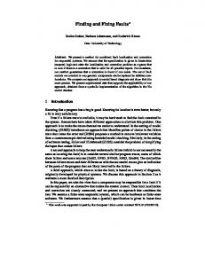
Inappropriate Uses of 3PLM One reason for the IRT model’s rise in popularity in a relatively short time in the measurement field was that the item parameters were easy to interpret and useful for item analysis. In the earliest IRT models such as 2PLM and 1PLM, the b- and a-parameters could be interpreted as item difficulty and item discrimination in general. 2 Once developed, 3PLM quickly became the dominant model for analyzing the MC item type because it often showed better model-data fit with MC items than did less flexible models such as 1PLM or 2PLM. In early usage of 3PLM, the c-parameter was directly interpreted as a guessing parameter, but as later research revealed, the cparameter estimates tended to differ from those resulting when an examinee had made a completely random guess (Lord, 1974). A more appropriate term for c-parameter was proposed–‘pseudo-guessing parameter’ (Hambleton et al., 1991). The a- and b- parameters of 3PLM, however, are still widely called and interpreted respectively as item discrimination and item difficulty, as in 2PLM. This poses the question: “Should the a- and bparameters of 3PLM also be interpreted as ‘pseudodiscrimination’ and ‘pseudo-difficulty’ parameters?” The fact that different combinations of a-, b-, and cparameters could result in similar IRFs for the part of the theta scale where the majority of test scores are distributed is well known in the field. Figure 2 presents an example of such a case in which the item parameter Some experts may reasonably argue that those items that have the same b-parameters but different aparameters would result in different response probability (RP) across the theta scale. So the b-parameter can be interpreted as item difficulty only when 1PLM or the Rasch (1960) model is used. While that point of view is not invalid, the b-parameter of 2PLM still can be seen correctly reflecting item difficulty on average across theta scale.

2

Page 6 values for Items 1, 2, 3, and 4 differ substantially, even though the IRFs of those items resemble each other when –1< θ < 1 (the unshaded area), where a majority of examinees are found. On the other hand, even though Items 3 and 5 have the same value for the b-parameters, their IRFs show considerably different item characteristics, especially in terms of practical difficulty. Thus, a-, b-, and c-parameters of 3PLM should not be interpreted individually but rather analyzed together, for example, in a form of IRF. This example may be stating the obvious to those who have sufficient experience with 3PLM, but applications and practices that use item parameters with 3PLM inappropriately are observed with some frequency in the field of educational and psychological measurement. For example, in an item analysis process, test items often are ordered by bparameter regardless of a- and c-parameters and inappropriately considered as if the items were sorted exactly by item difficulty. In differential item functioning (DIF) or item parameter drift (IPD) analyses, DIF detection methods originally developed for 1PLM—Chi-square tests for example (Lord, 1980)—are occasionally applied only to a- or b-parameters of 3PLM without an appropriate modification. In test equating, some of the linear transformation methods—the mean-mean and mean-sigma methods of Loyd & Hoover (1980) and Marco (1977)—use only aand/or b-parameter estimates to compute the linking coefficients. Even with the test characteristic curve (TCC) methods (Haebara, 1980; Stocking & Lord, 1983), the linking coefficients are not applied to the c-parameter estimates, so these estimates are left untransformed (Han, Wells, & Hambleton, 2009). Unfortunately, some practitioners in the field habitually have used 3PLM item parameters inappropriately, unaware of or unconcerned about their consequences. Some misuse of item parameters, in fact, has had little impact and thus can be ignored. In other cases, however, the consequences for item evaluation are unacceptable. For example, the bookmark or itemmapping methods (Lewis, Green, Mitzel, Baum, & Patz, 1998) for standard setting could be a sound approach when 1PLM is used because items can be ordered correctly by difficulty using the b-parameter. When 2PLM is used, items are ordered instead by location at RP = 0.67 according to P(θ) = (2 + c)/3 with c being zero because that is where items result in the maximum information (Huynh, 1998). With 3PLM, however, assuming c ≠ 0, the use of P(θ) = (2 + c)/3 would result in several different RP values for item evaluation unless all items had a common c-parameter value. To resolve

Practical Assessment, Research & Evaluation, Vol 17, No 1 Han, Fixing c Parameter in 3PLM this issue in practice, c-parameter values of items often are simply adjusted to be zero (Cizek & Bunch, 2007; Lorié, Egan, Mercado, Brandstrom, & Tele’a, 2004). Such practice might be acceptable if c-parameter values were very close to zero and the differences in c-parameter values among items were negligible. For items whose cparameter values vary greatly from zero, however, adjusted IRFs could result in substantially deflated RP values and the order of items could be significantly changed. As a result, the cut scores determined by the RP value could be seriously misleading.

Item 1 a = 1.00 b = –1.00 c = 0.20

Item 2 a = 1.10 b = –0.90 c = 0.25

Item 3 a = 0.95 b = –1.10 c = 0.15

Item 4 a = 1.10 b = –0.80 c = 0.33

Item 5 a = 1.10 b = –1.10 c = 0.25

Figure 2. An example of items resulting in similar IRFs The best way to prevent undesirable consequences of such misuse of the item parameters with 3PLM simply would be not to use or not to interpret the item parameters. Graphical analyses on IRFs could be used instead. Preventing the 3PLM item parameters from being interpreted, however, would substantially limit the utility of 3PLM. A more practical solution would be to replace the 3PLM with other models, the parameters of which can be interpreted. As discussed earlier, since the (random) guessing and problem-solving processes are conceptually distinguished in FG3PLM, and because the c-parameter of FG3PLM is fixed as long as the number of multiple choices is consistent, then the a-, b-, and cparameters can be directly interpreted as discrimination, difficulty, and guessing with FG3PLM. Thus, FG3PLM can be a viable alternative to 3PLM when each item parameter needs to be interpreted and used for other purposes.

Utility Versus Flexibility The advantage that FG3PLM offers in allowing for more meaningful interpretation of the a-, b-, and c-

Page 7 parameters than found in 3PLM is offset by a possible tradeoff in flexibility. Since FG3PLM mathematically is a special case of 3PLM (even though each model starts from different conceptualizations of the problem-solving and guessing processes), the IRFs using FG3PLM would be less flexible than 3PLM and potentially would have a negative impact on the model-data fit. Therefore, the first research question to be answered is: “How different is FG3PLM from 3PLM in model fit with various educational data?” Several studies have examined the model fit comparing 3PLM with 2PLM and/or 1PLM (Swaminathan & Gifford, 1979; Hambleton & Murray, 1983; Hambleton et al., 1991). These studies concluded that 3PLM provided much better model fit over 2PLM and/or 1PLM. Other studies compared 3PLM with other IRT models similar to FG3PLM in equating context with simulated data (Marco, Wingersky, & Douglass, 1985; Way & Reese, 1991), but few studies actually applied both 3PLM and FG3PLM to various educational data and evaluated model fit. The first study (Study 1) of this paper will apply both 3PLM and FG3PLM to three different sets of response data from various educational settings and testing populations and examine their differences in terms of model-data fit.

Stability and Accuracy Several parameter estimation techniques with 3PLM, such as joint maximum likelihood estimation (Birnbaum, 1968; Lord, 1974, 1980) and marginal maximum likelihood estimation, or MMLE (Bock & Lieberman, 1970; Bock & Aitkin, 1981), were developed and became available with computer programs. An extensive number of studies followed that further contributed to existing knowledge about parameter estimation with 3PLM (Lord, 1975; Lord, 1983; Thissen & Wainer, 1982; Wingersky & Lord, 1984; Lord & Wingersky, 1985; Baker, 1967, 1986; McKinley & Reckase, 1980; Swaminathan & Gifford, 1986). This research mainly studied model-data fit, parameter recovery, and/or standard error and bias of estimation. Studies found several factors that affected the estimation results (e.g., sample size, test length, item characteristics, and distributions). One issue raised repeatedly by several studies was the difficulty of estimating the c-parameters of 3PLM. Estimating the c-parameters (which are derived from the lower asymptote of an item characteristic function) is hard to do in practice, especially when an item is either very easy (low b-parameter) and/or does not discriminate well (low a-parameter) due to the fact

Practical Assessment, Research & Evaluation, Vol 17, No 1 Han, Fixing c Parameter in 3PLM that there are few examinees at the point on the theta scale defined by the lower asymptote (Lord, 1975, 1980; Baker 1967; McKinley & Reckase, 1980). As a result, cparameter estimates tend to be less stable, with substantially larger standard errors, than a- and bparameter estimates, considering the difference in scale of each parameter. Despite these technical difficulties, 3PLM has been used as a primary IRT model for MC items because it results in much better model fit than found with 2PLM or 1PLM. If the first study in this paper were to show that FG3PLM resulted in acceptable model fit with various MC item data, then it would be used to solve the problems with the c-parameter estimation of 3PLM. With FG3PLM, c-parameters are computed based on what is already known—the number of answer options of an MC item—so there would be no stability issues in the cparameter estimation. All response data could be used to estimate a- and b-parameters, resulting in more stable aand b- parameter estimation than with 3PLM. The second study (Study 2) in this paper, therefore, will employ a series of simulation studies to evaluate the estimation stability (i.e., standard error of estimation) of both 3PLM and FG3PLM in various conditions including number of options of MC items, sample size, shape of distribution, model choice, and sparseness of response matrix. Study 2 will also examine the estimation accuracy (i.e., bias of estimation) with both models.

Study 1: Model Fit Study With Real Data Sets

Research Design This study analyzed real data sets from three different testing programs to evaluate model-data fit with 3PLM and FG3PLM. The first response data set (Data Set 1) came from a statewide 10th-grade geometry assessment given as a high school graduation requirement. The test consisted of 31 MC items and was administered to 6,123 examinees. Each item had four options. The second data set (Data Set 2) was from another statewide assessment, a third-grade English Language Arts (ELA) exam given as part of the “No Child Left Behind” (NCLB) federal testing requirements. This test consisted of 40 MC and two open-response (OR) items and was administered to about 70,000 examinees. Each MC item had four options. The third data set (Data Set 3) was from a verbal exam administered through a computerized adaptive testing (CAT) program as a graduate-level standardized admissions test. The CAT data consisted of hundreds of

Page 8 items, and a test tailored to each examinee consisted of 41 MC items, some of which were calibrated and equated using the fixed common item parameter (FCIP) method.3 Only those nonoperational, pretest items, which were not adaptively administered, were included in the analysis after the item calibration. Only a portion of the item set was administered to each individual examinee and the full response matrix was 77.6 % sparse with about 17,000 examinees. Each MC item had five options. For Data Sets 1 and 2, PARSCALE (Muraki & Bock, 2003) computer software was used to estimate item parameters with 3PLM and FG3PLM. 4 PARAM3PL (Rudner, 2005) was used for Data Set 3. As for FG3PLM, c-parameters for MC items were fixed to the statistical probability of getting points completely by random guessing (i.e., 0.25 for the first and second data sets, which had four options, and 0.20 for the third data set, which had five options). To evaluate data-model fit of the three data sets with 3PLM and FG3PLM, chi-square statistics were used, as well as visual investigation of the raw and standardized residual plots using computer software ResidPlots-2 (Liang, Han, & Hambleton, in press). Chisquare statistics were computed as follows: K

N j (Oij − E ij ) 2

j =1

E ij (1 − E ij )

χ i2 = ∑

(3)

where Nj is the number of examinees in score interval j; Oij is the observed proportion of examinees in interval j who answer item i correctly; and Eij is the probability based on the model in interval j answering item i correctly. Degree of freedom equals number of score intervals minus the number of parameters being estimated. The study also evaluated standard error (SE) of estimation for each item parameter to examine stability of item parameter estimation.

Results Table 2 displays item parameter estimates for 3PLM and FG3PLM with Data Set 1(10th-grade geometry test). This data set is not used to calibrate the operational item parameters for that program. 4 The item parameters were estimated using the MMLE method with the logistic model based on a scale constant of 1.7. A log-normal distribution and a normal distribution were used as prior distributions for a- and bparameters, respectively. No distribution was assumed for c-parameters.   3

Practical Assessment, Research & Evaluation, Vol 17, No 1 Han, Fixing c Parameter in 3PLM The average of c-parameter estimates with 3PLM was 0.251, which was very close to 0.250 with FG3PLM. The mean differences in a- and b- parameter estimates between 3PLM and FG3PLM were also minimal (< 0.1). The standard errors (SE) of item parameter estimation, however, differed moderately between 3PLM and FG3PLM, considering the scales of each parameter. Since the c-parameter was not estimated but fixed with FG3PLM, the mean SE for the c-parameter was zero, while it was 0.030 with 3PLM. The mean SE values for the a- and b-parameters were also larger with 3PLM than with FG3PLM probably because of the SE of cparameter estimation. Table 2. Comparisons of Item Parameter Estimates Between 3PLM and FG3PLM Parameter Data Set 1 6,123 Examinees (Grade 10) 31 MC Items

a

Data Set 2 70,282 Examinees (Grade 3) 40 MC + 2 OR Items

a

Data Set 3 17,023 Examinees (Higher Ed) 78 Items (77.6% sparse)

b c

b ca) a b c

Mean (SE) 0.066 0.050 0.101 0.041 0.030 0.000 0.020 0.013 0.018 0.010 0.011 0.000 0.135 0.128 0.061 0.064 0.029

SD (SE) 0.018 0.022 0.191 0.037 0.048 0.000 0.006 0.004 0.008 0.004 0.003 0.000 0.107 0.099 0.027 0.028 0.012

Model

Mean

SD

3PLM FG3PLM 3PLM FG3PLM 3PLM FG3PLMb) 3PLM FG3PLM 3PLM FG3PLM 3PLM FG3PLMb) 3PLM FG3PLM 3PLM FG3PLM 3PLM

1.154 1.094 0.066 0.020 0.251 0.250 1.301 1.087 –0.653 –0.815 0.260 0.250 1.118 1.063 –0.206 –0.223 0.198

0.447 0.478 1.043 1.064 0.089 0.000 0.367 0.324 0.388 0.499 0.071 0.000 0.582 0.568 1.014 1.020 0.137

FG3PLMb)

0.200 0.000 0.000 0.000

Only MC items were included in the statistics. b) Standard error of c-parameter estimation was all zero with FG3PLM because c-parameters were not estimated but fixed to either 0.25 or 0.20 in accordance with the number of options of the MC items. a)

Figure 3 summarizes the chi-square fit indices for each item.5 The changes in model-data fit from 3PLM to FG3PLM were minimal for most items. Items 3 and 23 The significance test using the chi-square fit statistics was skipped in this study because the chi-square test is not effective (resulting in a high Type I error rate) when the sample size is large.

5

Page 9 showed substantial increases in the chi-square value with FG3PLM. As shown in Figure 4, Item 3 with FG3PLM had moderate raw residuals in the lower theta area due to some observed data that were not along the expected IRF. On the other hand, Item 3 had much smaller residuals with 3PLM because the lower asymptote of the IRF could be adjusted by a much smaller c-parameter estimate (0.088) for 3PLM. Item 23, the c-parameter estimates of which were 0.091, also showed the residual patterns similar to Item 3. Thus, it seemed that substantial changes in chi-square fit index between 3PLM and FG3PLM tend to occur when c-parameter estimates for 3PLM are much lower than ones for FG3PLM. To understand the overall residuals across items, the frequency distributions of standardized residuals for 3PLM and FG3PLM were compared. In Figure 5, FG3PLM showed slightly more negative standardized residuals than 3PLM, but the overall difference between 3PLM and FG3PLM was not very meaningful. In short, the differences in item parameter estimates and model fit between 3PLM and FG3PLM with Data Set 1 were minimal except for the two items.

Figure 3. Data-model fit indices (chi-square) for items of test data 1. With Data Set 2 from the third- grade ELA exam, the average c-parameter estimate with 3PLM was 0.260, which differed slightly from 0.250 with FG3PLM (Table 2). It should be noted that the average of a- parameter estimates also differ by 0.214 between 3PLM and FG3PLM and was consistent with van der Linden and Hambleton’s results (1997),where small changes in the cparameter could be compensated by small changes in the a-parameter. There also were moderate differences in the average b-parameter estimates between models, probably because partial knowledge was reflected in the cparameter estimates with 3PLM (San Martin et al., 2006).

Prractical Assessm ment, Research & Evaluation, Vol V 17, No 1 H Han, Fixing c Parameter P in 3PLM 3

Page 10

Iteem 3 (Poor Fitt) with FG3PL LM (aa=1.999, b=0.9667, c=0.250)

Item 3 (Good Fit) F with 3PLM M (a=1.409, b=00.749, c=0.088)

Figure 6. Data-modeel fit indices ((chi-square) fo or items of test daata 2

Fi Figure 4. An exaample item off poor data-m model fit for teest daata 1 with FG G3PLM

Figure 7. Frequency distribution o of standardizeed residuals for daata set 2

Fi Figure 5. Frequeency distributiion of standarrdized residualls fo or data set 1 The chi-sqquare fit statisstics showed similar pattern ns w with the Data Set 1 (Figure 6). There were w two item ms (IItems 14 and 39) 3 that show wed poor fit to o FG3PLM, an nd th hose items had d very low c-p parameter estiimates (0.16 for f Ittem 14 and 0.113 for Item 399) with 3PLM M. Overall, theere w were slightly more m positive standardized d residuals wiith 3P PLM, and slightly more negative residuals wiith FG G3PLM in comparison, but the diffferences weere m minimal (Figuree 7).

T The two OR ittems (Item 411 and 42) weree calibrated with Muraki’s (1992) generaliized partial ccredit model M). As shownn in Table 3, w when FG3PLM M replaced (GPCM 3PLM M for the MC items, the a--parameter esttimates for the O OR items decreased sligh htly as the aa-parameter estimaates for the MC items were decreased. Th he standard deviatiion (SD) of b--parameter esttimates for thee OR items also chhanged as thee SD of b-paraameter estimaates for the MC iteems. Althouggh it may be imprudent to o generalize about the item paraameter estimattes between th he MC and G3PLM replaces 3PLM (or vvice versa), OR iteems when FG it is w worth noting that a choicee of model fo or the MC items aalso influencees the item parrameter estimaates for the OR iteems. Inn the case of Data Set 3, eeach examineee sitting for a gradduate-level addmissions tesst took only a portion (aboutt 22.4%) of nnon-precalibraated items thaat were not adaptivvely adminisstered. Exam minee proficiiency was estimaated using oother items that were adaptively admini nistered, and tthose proficieency estimatess as well as

Prractical Assessm ment, Research & Evaluation, Vol V 17, No 1 H Han, Fixing c Parameter P in 3PLM 3

Page 11

th he response data were used u to estim mate the iteem paarameters of the non-precaalibrated item ms. As shown at th he bottom of o Table 2, the average values of th he paarameter estim mates between n 3PLM and FG3PLM weere cllose. Standard d errors of estimation e (SEE) were also cllose except forr the c-parameeter. Regardingg the chi-squuare fit statisstics, no item ms in ndicated a draamatic increasse from 3PLM M to FG3PLM M (F Figure 8). Som me items fit better b with 3P PLM; others fit beetter with FG G3PLM, but the t change in n the chi-squaare vaalues was insuubstantial for most items. As A a result, th he diistribution off the standard dized residuaals from 3PLM an nd FG3PLM also a was similaar. (Figure 9).

Figure 99. Frequency distribution o of standardizeed residuals for datta set 3

Stu dy 2: Para ameter Rec covery Stud dy with S Simulated Data

Reseaarch Design n

Fi Figure 8. Data-m model fit indicces (chi-squaree) for items off teest data 3 Data Sets 1, 2, and 3 represented three different sttudent populations: high K--12, low K-122, and graduatteleevel education n. Each data set s also repressented different teesting applicattions: MC item ms only, MC and OR item ms m mixed, and com mputer-based d testing (CBT T), respectivelly. A Across the dataa sets, the cho oice of model between 3PLM an nd FG3PLM rarely r had an impact i on thee model-data fit. f The differencees in a-, b-, and c-param meter estimattes beetween the two modeels also weere negligiblle. In nterestingly, th he average c-paarameter estim mates for 3PLM w were close to 1/k with k beiing the numbeer of options of th he MC items. It seemed wh hat Lord (19774) pointed ouut, th hat c-parameteer estimates teend to be sm maller than 1/ /k, diid not necessarily hold true, at least witth the data seets an nalyzed in Sttudy 2, when n using the latest computter prrograms for item i parametter estimation n and especiallly w when sample size s was largee. Analyses off the three reeal daata sets lead ds to the co onclusion thaat the use of FG G3PLM could offer decen nt model-data fit comparab ble to o 3PLM.

SStudy 2 emplooyed simulateed data sets tto examine item pparameter estim mation accuraacy and stabiliity between 3PLM M and FG3PL LM. Since SStudy 1 already found evidennce supportingg satisfactory model fit of b both 3PLM and F FG3PLM to ttest response data sets fro om various educattional settingss, model fit w was not a maiin focus in Study 2. The respoonse data werre simulated ffor 40 MC items and the numbber of examin nees varied byy condition (300, 6600, 1,000, aand 2,000) folllowing eitherr a normal distribbution with a mean of 0 aand a standardd deviation (SD) oof 1 or a unifo form distributiion that rangeed between –3 andd 3. True c-paarameter valuues were set to o 0.2, 0.25, and 0..5 by conditiion to mimic five-option MC items, four-ooption MC items, and true-false tyype items, respecctively. The ssparseness of response maatrices also was vaaried by conddition (0%, 255%, 50%, and 75%), and the unnpresented iteems were cho osen randomlly for each individdual. As for the parameter estimation, noncoonverged calibbrations were handled sepaarately and not inncluded in thee main result.. Once item parameters were ccalibrated,6 the study evaluuated estimatio on stability and acccuracy for aa-, b-, and c- parameters uusing mean standaard errors of eestimation (SE EE), root meean squared error ((RMSE), and BIAS statisticcs to summariize random The ssame estimation method an nd options thaat were used w with the real ddata analyses w were used again n with one excepttion: The distrribution optio on was modifieed accordding to the corrresponding trrue sample disstribution (norm mal or uniform)). 6

Practical Assessment, Research & Evaluation, Vol 17, No 1 Han, Fixing c Parameter in 3PLM

Page 12

and systematic errors. RMSE and BIAS were computed as follows (e.g., for a-parameter): R

RMSEai =

∑ (aˆ

ir

r =1

− ai )

2

(4)

R and R

BIASai =

∑ (aˆ r =1

ir

− ai )

(5)

R

where aˆir and ai represent the a-parameter estimate of rth replication and true value for item i, respectively. R represents the number of replications. The 40 MC items were classified into three groups by true b-parameter value or difficulty (e.g., the 10 easiest items, the 10 hardest items, and the 20 items in the middle) and also by true a-parameter value (discriminating power). The item parameter estimation results were summarized by group to investigate the effect of item characteristics on parameter estimation. The effect of test length was also studied. The original 40 items were used twice to simulate the conditions with a doubled test length (80 items), and, at the same time, to control other extraneous factors. Table 4 shows the statistics for the true characteristics of the items grouped by difficulty or discrimination. The data simulation was accomplished using computer software WinGen (Han, 2007), and each condition was replicated 100 times. PARSCALE (Muraki & Bock, 2003) computer software was used to estimate item parameters with 3PLM and FG3PLM.7 The total number of simulations in the study was 38,400 (= 4 sample sizes x 3 true c-parameter values x 2 distributions x 4 sparseness x 2 test length x 2 IRT models x 100 replications).

The choice of estimation method and option was consistent throughout the analyses of the real and simulation data. The convergence criterion for the EM cycle was to reach 0.01 (change in log likelihood value) within 1,000 iterations. Unsuccessful item calibrations due either to nonconvergence or mathematical error were summarized separately and excluded from the main results. The option for examinee distributions (normal or uniform) was chosen in accordance with corresponding true distribution and the scale of estimates was also transformed accordingly for comparison with the true parameters.

7

Table 4. Descriptive Statistics for True Item Parameters for Each Item Group Items Grouped by ParaN Discriminating meter Power Lower 10 a b Mid 20 a b Higher 10 a b Items Grouped by ParaDifficulty N meter Easier 10 a b Mid 20 a b Harder 10 a b Total 40 a b

Mean

SD

Min

Max

0.707 0.116 1.235 –0.164 2.346 –0.058

0.135 0.466 0.865 1.079 –2.166 1.319 0.234 0.888 1.625 1.004 –2.277 2.180 0.450 1.688 3.152 1.219 –1.677 2.467

Mean 1.523 –1.423 1.331 –0.001 1.337 1.154 1.381 –0.068

SD Min Max 0.787 0.682 3.152 0.521 –2.277 –0.899 0.540 0.466 2.628 0.448 –0.835 0.485 0.812 0.531 2.787 0.660 0.553 2.467 0.667 0.466 3.152 1.057 –2.277 2.467

Feasibility To evaluate the feasibility of using the models in practice, Study 2 investigated the percentage of cases with successfully converged item calibration across 100 replications within each condition. The first thing to notice in Figure 10 is the difference between 3PLM and FG3PLM. The 3PLM simulations yielded a low percentage of successful item calibrations, especially when the sample size was small (e.g., n = 300), the theta distribution was normal, and/or the true c-parameter was large (e.g., c = 0.50). On the other hand, FG3PLM showed much a higher convergence rate across conditions even with smaller samples (n = 300, 600). Regarding the shape of distribution, both 3PLM and FG3PLM worked much better with the uniform distribution than with the normal distribution. In particular, the convergence rate of 3PLM with the uniform distribution was dramatically improved compared with the normal distribution conditions when the sample size was relatively small. This was due to a greater number of individuals with a lower proficiency level under the uniform distribution compared with the same sample size under the normal distribution. This was consistent with what Lord and Wingersky (1985) discovered. When c = 0.50, however, the improvement

Practical Assessment, Research & Evaluation, Vol 17, No 1 Han, Fixing c Parameter in 3PLM

Page 13

Figure 10. Percentage of successfully converged estimations

of the convergence rate with 3PLM under the uniform distribution was limited. Test length heavily influenced the convergence rate with 3PLM as well. Under the studied conditions, the convergence rate with 3PLM dropped when the test length changed from 40 to 80. With FG3PLM, the effect of test length on the convergence rate was small. The impact of the sparseness of response matrices on the convergence rate was also

studied under each condition, but there were heavy interactions among sample size, test length, and sparseness, and it was hard to identify the consistent main effect of sparseness across conditions. The findings shown in Figure 10 lead to the conclusion that the applications with 3PLM would be feasible only when MC items having a sufficient number of options (i.e., c < = 0.25) are calibrated with a large

Practical Assessment, Research & Evaluation, Vol 17, No 1 Han, Fixing c Parameter in 3PLM sample (> 1,000) or with a uniformly distributed sample. In addition, the convergence rate with 3PLM was heavily influenced by the interactions between test length and sparseness of a response matrix. FG3PLM turned out to be a much more feasible application even with a small sample size; plus it worked well with MC items that had few options (e.g., c = 0.50 like the true-false item type).

Stability of Item Parameter Estimation The stability of item parameter estimation was evaluated based on the standard errors of estimation (SEE). As shown in Figure 11, the choice of model had the greatest impact on the SEE. Throughout the studied conditions, FG3PLM resulted in much lower SEEs compared with 3PLM, even with small samples. Since cparameters were fixed with FG3PLM, SEEs for cparameters were always zero. Although the a-parameter estimates were known to be closely related to c-parameter estimates (Lord, 1975), it was noteworthy that the SEEs for a-parameter did not seem to be influenced by the SEEs for c-parameter. In other words, there was no meaningful difference in the SEEs for a-parameter between 3PLM and FG3PLM. Instead, the SEEs for bparameter were dramatically increased as the SEEs for cparameter got larger with 3PLM, especially when the sample size was small and/or the sparseness was serious. It also should be noted that the SEEs with 3PLM were substantially lowered when the sample was uniformly distributed. In conclusion, 3PLM could result in relatively stable item estimates only when the sample size was very large (> 2,000) and the sparseness of the response matrix was none to minimal. On the other hand, FG3PLM offered very stable parameter estimation even with smaller samples (> 600) with moderate sparseness (25% to 75%). Test length and true c-parameter value showed little impact on the parameter estimation stability across the studied conditions.

Accuracy of Item Parameter Estimation Study 2 assessed the accuracy and bias of item parameter estimation using the BIAS statistic (Equation 5). As with a-parameter estimation, the sample distribution seemed to cause significant differences in BIAS (Figure 12). When the samples were normally distributed, the a-parameter estimates became more accurate as the sample size increased regardless of the choice of response model. When the sample distribution was uniform, however, the a-parameters were

Page 14 substantially underestimated with both 3PLM and FG3PLM, even with a large sample size. On the other hand, the c-parameter estimates were much less biased with the uniform distribution compared with the normal distribution (3PLM). As for the b-parameter estimates, the shape of distribution did not seem to be an important factor. Rather, the bias of b-parameter estimates varied greatly across sample size and choice of the response model. The bias in the b-parameter estimation was minimized when the sample size was 600 or larger with FG3PLM or when it was 2,000 with 3PLM. The sparseness of response matrix seemed to influence the bias of the item parameter estimates, but it was difficult to interpret because of the complicated interactions among the other factors. To conduct a deeper investigation of the main causes of the bias of the item parameter estimates, all 40 items were classified into one of three groups either by true a- parameter (discrimination) or by true b-parameter (difficulty) value (Table 4). As shown in Figure 13, the bias in a-parameter estimates was minimal and not meaningfully different across the studied conditions when the true item discrimination was low to mid-range. For those items with higher discrimination, however, the a-parameter estimates tended to be substantially underestimated when the sample was too small (< 2,000) or when the response matrix was severely sparse (> 50%). This probably was due to the fact that the a-parameter scale is logarithmic, which means both the systematic and random errors of a-parameter estimation became larger as the parameter value increased. Also, it should be noted that the a-parameters were noticeably underestimated when the sample was uniformly distributed. In terms of choice of IRT model, there seemed to be no meaningful difference between 3PLM and FG3PLM. Figure 14 shows the bias of the b-parameter estimates. When the sample was normally distributed, the bias was minimized with FG3PLM with the sample size equal to or larger than 600 regardless of the true item discrimination and difficulty. With 3PLM, on the other hand, the b-parameter estimates exhibited a large degree of bias, even with the large sample (n = 2,000) when the true item discrimination was not in the mid-range and/or the true item difficulty was lower. This result is similar to the findings on 3PLM in Thissen and Wainer (1982). When the sample distribution was uniform, however, both 3PLM and FG3PLM yielded b-parameter estimates that were either overestimated for harder items or

Practical Assessment, Research & Evaluation, Vol 17, No 1 Han, Fixing c Parameter in 3PLM

Figure 11. Stability of item parameter estimation with 3PLM and FG3PLM

Page 15

Practical Assessment, Research & Evaluation, Vol 17, No 1 Han, Fixing c Parameter in 3PLM

Figure 12. Accuracy of item parameter estimation with 3PLM and FG3PLM

Page 16

Practical Assessment, Research & Evaluation, Vol 17, No 1 Han, Fixing c Parameter in 3PLM

Figure 13. Bias of a-parameter estimation by item discrimination and difficulty

Page 17

Practical Assessment, Research & Evaluation, Vol 17, No 1 Han, Fixing c Parameter in 3PLM underestimated for easier items. It is important for practitioners to keep in mind that when the shape of proficiency distribution is (or at least expected to be) close to a rectangle (like the uniform distribution), the chance of obtaining biased b-parameter estimates could be considerable both for easier and harder items. Last, we see the bias of the c-parameter estimates, as illustrated in Figure 15. Since the c-parameters were not estimated but fixed with FG3PLM, there was no bias in this sample. With 3PLM, however, the c-parameter estimates were inaccurate when the sample was normally distributed and too small (≤ 600). Even with a large sample, there was a high level of bias in c-parameter estimates for items with low discrimination and/or easy difficulty. For example, when the discrimination was low and the item difficulty was easy (the first cell at the top of Figure 15), the mean bias of the c-parameter estimates for those items often exceeded 0.20. Considering that the scale of c-parameter ranges between 0 and 1, estimates with such bias cannot be accepted in practical usage. As for proficiency distribution, Figure 15 shows that the bias of the c-parameter estimates was moderately reduced when the sample distribution was uniform in comparison with the normal distribution condition. The accuracy of the c-parameter estimates for easy items with lower to mid-discrimination was still unacceptably poor to be useful in practice, however, even when the sample was uniformly distributed. The bias statistics for a-, b- and c-parameter estimates in 3PLM showed that they were heavily influenced by each other (especially by biased cparameter estimates) so interpreting a-, b-, and cparameter estimates separately when 3PLM is in use could yield misleading results.

Summary and Discussion The 1970s, ‘80s and ‘90s saw an extensive number of studies conducted to understand technical problems associated with 3PLM. Many of these studies, however, examined only a few factors (or just a single factor) that play a key role in 3PLM estimation. Because computer technology and estimation techniques for IRT models have changed so significantly since the 1990s, we decided the time was right to conduct a series of comprehensive simulation studies to revisit these earlier findings and determine whether they were still relevant to today’s much more complicated test designs. Simulation Study 2 discovered several conditions that can make estimating item parameters for 3PLM technically challenging—some of them concurred with

Page 18 previous findings and some were new. The item parameter estimation procedure using the maximum likelihood estimation method often was unsuccessful in obtaining converged estimates when the true c-parameter value was large (> 0.25) and/or when the sample size was small, especially with longer test length8 (Figure 10). Even if the converged estimates were obtained successfully, the SE of b- and c- parameter estimates was too large to be practical when the sample size was small (< 2,000) and/or sparseness of the response matrix was moderate (> 50%) (Figure 11). On a more critical level, the accuracy of c-parameter estimates for items that were neither hard nor very discriminating was far from satisfactory to be of use in practice (Figure 15). Similar problems in estimating c-parameters had been reported in earlier studies (Lord, 1974; Wood, Wingersky, & Lord, 1976; Thissen & Wainer, 1982). It was interesting to learn what little progress has been made in the last 30 years to improve the SE and accuracy of c-parameter estimation, even with the availability of advanced computer programs and sophisticated estimation algorithms. It lead us to what Holland (1990) concluded: A one-dimensional test can only support two parameters per item, and so, 3PLM just might be overparameterized. If the c-parameter cannot be estimated, 3PLM does not exist (Wright, 1977). Therefore, it may be correct to conclude that 3PLM simply may be unrealistic (except in the unlikely case where all items are well discriminating, sufficiently difficult, and administered to an extremely large number of test takers). Unfortunately (yet convenient perhaps for some), there are still available a handful of computer programs that can provide practitioners with 3PLM parameter estimates even when 3PLM statistically is impossible. For example, many computer programs for item calibration provide approximate parameter estimates even if the model is not satisfactorily converged. As for cparameters, most computer programs do not estimate the parameters when certain criteria for c-parameter estimation are not met, such as the index, ‘b-2/a,’ by Lord (1975). They still produce some values as cparameter estimates, which often are the average value of the c-parameters or a default value like zero. Many practitioners in the field remain inadequately informed

The iterative E-M procedure for item parameter estimation was stopped after 1,000 iterations (unless the change in log likelihood value met the criterion first, which was 0.01).  

8

Practical Assessment, Research & Evaluation, Vol 17, No 1 Han, Fixing c Parameter in 3PLM

Figure 14. Bias of b-parameter estimation by item discrimination and difficulty

Page 19

Practical Assessment, Research & Evaluation, Vol 17, No 1 Han, Fixing c Parameter in 3PLM about these problems associated the 3PLM calibration and, as a result, and are often misled into thinking that 3PLM works well and that c-parameter estimates are accurate as long as the computer programs output some values as parameter estimates. Even if 3PLM were estimated properly without any technical issues, 3PLM with c-parameter is no longer a member of logistic functions (Birnbaum, 1968) and loses many useful statistical properties (Baker, 1986). As shown earlier in Figure 2, a- and b- parameters are not comparable across items unless the items being compared have the same c-parameter value. In other words, a- and b- parameters of 3PLM cannot be interpreted as and/or used as indices for item discrimination and difficulty, respectively, when cparameter is freely estimated. The uncomfortable truth for practitioners to realize is that a-, b-, and c-parameters of 3PLM have little utility in item analysis unless the three parameters are viewed altogether in the form of IRF. Another critical problem with 3PLM, mentioned in the beginning of this article, is the ambiguity of the model’s definition of ‘guessing.’ Some researchers assume that all examinees, even those of varying proficiency levels, have the same capacity for or probability of guessing successfully (Birnbaum, 1968; Baker, 1986). Others theorized that guessing occurs mainly with examinees of low proficiency levels (Lord, 1974, 1975; Hambleton et al., 1991), and some argued that guessing is related to the proficiency level throughout the theta scale. The incongruence among those different points of view on the guessing parameter is due mainly to the different ways researchers interpret logical guessing, which many believe is what happens when a test taker’s knowledge is insufficient for correctly answering a test question. Traditionally viewed, logical guessing is part of the overall guessing process, but this supposition only makes it difficult to disentangle logical guessing from random guessing. This study proposed redefining the guessing and the problem-solving processes (Figure 1), and viewed logical guessing as a component of the problem-solving process. Based on this new concept of the guessing process, random guessing becomes the only remaining component of the guessing process. Thus, parameters for the guessing process can be easily set up in a response model using information that is already known and unbiased: the mathematical probability of random guessing, which is 1/k, with k being the number of multiple choices in the item. As pointed out earlier, the a-

Page 20 , b-, and c-parameters of FG3PLM—unlike 3PLM—are comparable across items (as long as the number of choices is consistent), and, as a result, can be directly interpreted as discrimination, difficulty and guessing, respectively. Since fixing the c-parameter might negatively influence the model fit, Study 1 attempted to fit FG3PLM to the real test data sets from three distinctly different test populations and compare it with 3PLM. The results of Study 1 showed no meaningful difference in model fit between 3PLM and FG3PLM, leading us to conclude that FG3PLM fit data from various educational applications as well as 3PLM. The advantages of FG3PLM over 3PLM were more obvious in the Study 2 simulation. Having one less parameter to estimate per item, FG3PLM yielded higher success rates in obtaining converged item parameter estimates (Figure 10) compared with 3PLM, especially when the sample size was small (≤ 600). Study 2 also revealed that FG3PLM is preferable over 3PLM in terms of the stability and accuracy of item parameter estimation. Estimating accurate lower asymptote (cparameter) for 3PLM is difficult if not impossible; whereas the c-parameter for FG3PLM can be computed easily based on unbiased and known information. At least within the newly revised definition of the guessing process (with FG3PLM), the mathematical probability of the random guess (1/k) would be the best guess at the guessing parameter. One might recall earlier studies reporting cparameter estimates below 1/k (Lord, 1974, 1975). This was not necessarily true, however, at least with the real data sets analyzed in this study. In Study 1, the average cparameter estimates for 3PLM were very close to 1/k or even slightly above 1/k (Table 1). The simulated data sets in Study 2 also showed that the c-parameters tended to be overestimated when the true a-parameter values were in low to middle ranges (Figure 15). Thus, it would be logical to assume that the observed bias of the cparameter estimates was due mainly to the compensation between a- and c-parameters during the estimation procedure, a finding also reported by Lord (1975). Lord’s attempt to explain c-parameter estimates below 1/k, in which he said “item writers try hard and successfully to provide alternative (wrong) responses that will be attractive to low ability examinees (1975, p. 29)” was indeed plausible only when the observed responses were considered. It should be noted that the lower asymptote of a response function begins at the negative infinite on the theta scale, not at a certain point on the theta scale where low-ability examinees are observed. Imagine there

Practical Assessment, Research & Evaluation, Vol 17, No 1 Han, Fixing c Parameter in 3PLM

Figure 15. Bias of c-parameter estimation by item discrimination and difficulty

Page 21

Practical Assessment, Research & Evaluation, Vol 17, No 1 Han, Fixing c Parameter in 3PLM were examinees with extremely low ability (near negative infinity on the theta scale). Those examinees would not have understood the test question or the multiple choice options at all, and, as a result, their only possible response would have been to make a random guess. Even in the traditional view of the guessing process with the typical 3PLM, the lower asymptote value (cparameter) theoretically should be of the probability of the successful random guess (1/k). Even if some observed scores from a few low-proficiency examinees resulted in c-parameter estimates below 1/k in practice, it is unlikely they would be meaningful because the estimates would be based on an extremely small sample number that might just be noise (Samejima, 2009). In sum, it is probably unnecessary to introduce a new term, FG3PLM, to the field simply to refer to the IRT model that is mathematically the same as 3PLM. When items are estimated with the fixed c-parameter, however, and the item parameters are interpreted according to the reconceptualized problem-solving and guessing processes, I suggest using “random chance parameter.” It is a more appropriate and meaningful interpretation of the c-parameter than “guessing” or “pseudo-guessing.”

References Baker, F. B. (1967). The effect of criterion score grouping upon item parameter estimation. British Journal of Mathematical and Statistical Psychology, 20, 227–238. Baker, F. B. (1986, April). Two parameter: The forgotten model. Paper presented at the annual meeting of National Council on Measurement in Education, San Francisco. Birnbaum, A. (1968). Some latent trait models and their use in inferring an examinee’s ability. In F. M. Lord and M. R. Novick (Eds.), Statistical theories of mental test scores (chaps. 17–20). Reading, MA: AddisonWesley. Bock, R. D., & Aitkin, M. (1981). Marginal maximum likelihood estimation of item parameters: Application of an EM algorithm. Psychometrika, 37, 29–51. Bock. R. D., & Lieberman, M. (1970). Fitting a response curve model for dichotomously scored items. Psychometrika, 35, 179–198. Cizek, G. J., & Bunch, M. B. (2007). Standard setting: a guide to establishing and evaluating performance standards on tests, Thousand Oaks, CA: Sage Publications.

Page 22 Haebera, T. (1980). Equating logistic ability scales by weighted least squares method. Japanese Psychological Research, 22(3), 144–149. Hambleton, R. K., & Murray, L. N. (1983). Some goodness of fit investigations for item response models. In R. K. Hambleton, (Ed.), Applications of item response theory. Vancouver, BC: Educational Institute of British Columbia. Hambleton, R. K., Swaminathan, H., & Rogers, H. J., (1991). Fundamentals of item response theory. Newbury Park, CA: Sage Publications. Han, K. T. (2007). WinGen: Windows software that generates IRT parameters and item responses. Applied Psychological Measurement, 31(5), 457–459. Han, K. T., Wells, C. S., & Hambleton, R. K. (2009, July). Impact of item parameter drift on pseudo-guessing parameter estimates and test equating. Paper presented at the annual meeting of the Psychometric Society, Cambridge, UK. Holland, P. W. (1990). The Dutch identity: A new tool for the study of item response models. Psychometrika, 55, 5–18. Hutchinson, T. P. (1991). Ability, partial information and guessing: Statistical models applied to multiple-choice test. Rundle Mall, South Australia: Rumsby Scientific Publishing. Huynh, H. (1998). On score locations of binary and partial credit items and their applications to item mapping and criterion-referenced interpretation. Journal of Educational and Behavioral Statistics, 23(19), 35–56. Kolen, M. (1981). Comparison of traditional and item response theory methods for equating tests. Journal of Educational Measurement, 18, 1–11. Lewis, D. M., Green, D. R., Mitzel, H. C., Baum, K., & Patz, R. J. (1998, April). The bookmark standard setting procedure: Methodology and recent implementations. Paper presented at the meeting of the 1998 National Council on Measurement in Education, San Diego, CA. Liang, T., Han, K., & Hambleton, R. K. (in press). Computer software for IRT graphical residual analyses, Applied Psychological Measurement. Lord, F. M. (1952). A theory of test scores. Psychometric Monograph, No. 7, 1952. Lord, F. M. (1974). Estimation of latent ability and item parameters when there are omitted responses. Psychometrika, 39, 247–264.

Practical Assessment, Research & Evaluation, Vol 17, No 1 Han, Fixing c Parameter in 3PLM Lord, F. M. (1975). Evaluation with artificial data of a procedure for estimating ability and item characteristic curve parameters. (Research Bulletin RB-75-33). Princeton, NJ: Educational Testing Service. Lord, F. M. (1980). Applications of item response theory to practical testing problems. Hillsdale, NJ: Erlbaum. Lord, F. M. (1983). Maximum likelihood estimation of item response parameters when some responses are omitted. Psychometrika, 48, 477–482. Lord, F. M., & Wingersky, M. S. (1985). Sampling variances and covariances of parameter estimates in item response theory. In D. J. Weiss (Ed.), Proceedings of the 1982 item response theory and computerized adaptive testing conference (pp. 69–88). Minneapolis, MN: University of Minnesota, Department of Psychology, Computerized Adaptive Testing Laboratory. Lorié, W. A., Egan. K. L., Mercado, R. L., Brandstrom, A. J., & Tele’a. D. (2004, April). A comparison of response probability and canonical pseudo response item locations: Implications for the bookmark standard setting procedure. Paper presented at the annual meeting of National Council on Measurement in Education, San Diego, CA. Loyd, B. H., & Hoover, H. D. (1980). Vertical equating using the Rasch model. Journal of Educational Measurement, 17, 179–193. Marco, G. L. (1977). Item characteristic curve solutions to three intractable testing problems. Journal of Educational Measurement, 14, 139–160. Marco, G. L., Wingersky, M. S., & Douglass, J. B. (1985). An evaluation of three approximate item response theory models for equating test scores. ETS Research Report 8546. Princeton, NJ: Educational Testing Service. Maris, E. (1995). Psychometric latent response models. Psychometrika, 60, 523–547. McKinley, R. L., & Reckase, M. D. (1980). A comparison of the ANCILLES and LOGIST parameter estimation procedures for the three-parameter logistic model using goodness of fit as a criterion (Research Rep. 80-2). Columbia, MO: University of Missouri, Educational Psychology Department, Tailored Testing Research Laboratory. Muraki, E. (1992). A generalized partial credit model: Application of an EM-algorithm. Applied Psychological Measurement, 17, 351–363. Muraki, E., & Bock, R. D. (2003). PARSCALE 4.1: IRT Item analysis and test scoring for rating-scale data

Page 23 [Computer software]. Chicago: Scientific Software, Inc. Rasch, G. (1960). Probabilistic models for some intelligence and attainment tests. Copenhagen, Denmark: Danish Institute for Educational Research. Rudner, L. M. (2005). PARAM-3PL calibration software for the 3 parameter logistic IRT model [Computer software]. http://edres.org/irt/param. Samejima, F. (2009, April). A wise use of noise parameter(s) in CAT for accurate latent trait estimation. Paper presented at the annual meeting of the National Council on Measurement in Education, San Diego, CA. San Martin, E. del Pino, G., & de Boeck, P. (2006). IRT models for ability-based guessing. Applied Psychological Measurement, 30(3), 183–203. Stocking, M. L., & Lord, F. M. (1983). Developing a common metric in item response theory. Applied Psychological Measurement, 7, 201–210. Swaminathan, H., & Gifford, J. A. (1979). Estimation of parameters in the three-parameter latent-trait mode. Laboratory of Psychometric and Evaluation Research (Report No. 90). Amherst, MA: University of Massachusetts. Swaminathan, H., & Gifford, J. A. (1986). Bayesian estimation in the three-parameter logistic model. Psychometrika, 51, 589–601. Thissen, D., & Wainer, H. (1982). Some standard errors in item response theory. Psychometrika, 47, 397–412. Tucker, L. R. (1946). Maximum validity of a test with equivalent items. Psychometrika, 11, 1–13. Van der Linden, W. J., & Hambleton, R. K. (1997). Handbook of modern item response theory. New York: Springer Verlag. Way, W. D., & Reese, C. M. (1991). An investigation of the use of simplified IRT models for scaling and equating the TOEFL test. TOEFL Technical Report TR-2. Princeton, NJ: Educational Testing Services. Wingersky, M. S., & Lord, F. M. (1984). An investigation of methods for reducing sampling error in certain IRT procedures. Applied Psychological Measurement, 8, 347–364. Wood, R. L., Wingersky, M. S., & Lord, F. M. (1976). LOGIST: A computer program for estimating examinee ability and item characteristic curve parameters (RM-76-6). Princeton, NJ: Educational Testing Service. Wright, B. C. (1977). Solving measurement problems with the Rasch model. Journal of Educational Measurement, 14, 97–166.

Practical Assessment, Research & Evaluation, Vol 17, No 1 Han, Fixing c Parameter in 3PLM

Page 24

Citation: Han, Kyung T. (2012). Fixing the c Parameter in the Three-Parameter Logistic Model. Practical Assessment, Research & Evaluation, 17(1). Available online: http://pareonline.net/getvn.asp?v=17&n=1

Note: The views and opinions expressed in this article are those of the author and do not necessarily reflect those of the Graduate Management Admission Council®.

Acknowledgements: The author wishes to thank Lawrence M Rudner, Fanmin Guo, and Eileen Talento-Miller of Graduate Management Admission Council® (GMAC®) for their valuable comments and support. The author also is grateful to Paula Bruggeman of GMAC® for review and comments.

Author: Kyung T. Han Graduate Management Admission Council 11921 Freedom Dr. Suite 300 Reston, VA 20190 KHan [at] gmac.com